global water availability is calculated by forcing the global hydrological model ... In the case of modified discharge, the net blue water demand for the year.
WATER RESOURCES RESEARCH, VOL. 47, W07517, doi:10.1029/2010WR009791, 2011
Global monthly water stress: 1. Water balance and water availability L. P. H. van Beek,1 Yoshihide Wada,1 and Marc F. P. Bierkens1,2 Received 23 July 2010; revised 14 April 2011; accepted 11 May 2011; published 12 July 2011.
[1] Surface fresh water (i.e., blue water) is a vital and indispensable resource for human water use in the agricultural, industrial, and domestic sectors. In this paper, global water availability is calculated by forcing the global hydrological model PCR‐GLOBWB with daily global meteorological fields for the period 1958–2001. To represent blue water availability, a prognostic reservoir operation scheme was included in order to produce monthly time series of global river discharge modulated by reservoir operations. To specify green water availability for irrigated areas, actual transpiration from the model was used. Thus, the computed water availability reflects the climatic variability over 1958–2001 and is contrasted against the monthly water demand using the year 2000 as a benchmark in the companion paper. As the water that is withdrawn to meet demand directly interferes with blue water availability along the drainage network, this paper evaluates model performance for three regimes reflecting different degrees of human interference: natural discharge, discharge regulated by reservoirs, and modified discharge. In the case of modified discharge, the net blue water demand for the year 2000 is subtracted directly from the regulated discharge, taking water demand equal to consumptive water use. Results show that model simulations of monthly river discharge compare well with observations from most of the large rivers. Exceptions are basins subject to large extractions for irrigation purposes, where simulated discharge exceeds the observations even when water demand is taken into account. Including the prognostic reservoir operation scheme results in mixed performance, with a poorer approximation of peak flows but with a marginally better simulation of low flows and persistence. A comparison of simulated actual evapotranspiration with that from the ERA‐40 reanalysis as a proxy for observed rates shows similar patterns over nonirrigated areas but substantial deviations over major irrigated areas. As expected, assimilated actual evapotranspiration over these areas includes water from alternative sources, whereas the simulations with PCR‐GLOBWB are limited by soil moisture, i.e., green water availability. On the basis of this evidence we conclude that the simulation provides adequate fields of water availability to assess water stress at the monthly scale, for which a separate validation is provided in the companion paper. Citation: van Beek, L. P. H., Y. Wada, and M. F. P. Bierkens (2011), Global monthly water stress: 1. Water balance and water availability, Water Resour. Res., 47, W07517, doi:10.1029/2010WR009791.
1. Introduction [2] The existing imbalance of water availability and water demand causes water scarcity to be one of the most pressing environmental issues in the world today. Water demand is defined here as the volume of water required by users to satisfy their needs. Surface fresh water is the most readily available resource to meet the water demand of agriculture (i.e., irrigation and livestock), industry, households and municipalities. We take surface fresh water as indicative of blue water availability and thus depart from its common definition [e.g., Falkenmark, 1997] that includes ground1
Department of Physical Geography, Utrecht University, Utrecht, Netherlands. 2 Unit Soil and Groundwater Systems, Deltares, Utrecht, Netherlands. Copyright 2011 by the American Geophysical Union. 0043‐1397/11/2010WR009791
water resources as well. Rather, we choose to include groundwater as a particular resource in order to identify regions that may experience dwindling availability in the future [Wada et al., 2011]. Despite the fact that the world population currently uses only 10% of the maximum available blue water in the form of river discharge on the global scale [Oki and Kanae, 2006], water stress occurs since water availability is highly variable over space and time [Postel et al., 1996]. Meigh et al. [1999] noted that water scarcity often first becomes apparent as occasional deficits during periods of high demand or below‐average rainfall and may affect a narrow region only. As water availability and demand vary over time, water stress may be underestimated by annual assessments as availability and demand may be out of phase. Therefore, the objective of this study is to quantify at a monthly time scale the seasonal and interannual variations in blue water stress on the global scale when water demand is confronted with climate‐induced
W07517
1 of 25
W07517
VAN BEEK ET AL.: GLOBAL MONTHLY WATER STRESS, 1
Figure 1. Model concept of PCR‐GLOBWB [van Beek and Bierkens, 2009]. The left‐hand side represents the vertical structure for the soil hydrology representing the canopy, soil column (stores 1 and 2), and the groundwater reservoir (store 3). Precipitation (PREC) falls as rain if air temperature (T) is above 0°C and as snow otherwise. Snow accumulates on the surface, and melt is temperature controlled. Potential evapotranspiration (Epot) is broken down into canopy transpiration and bare soil evaporation, which are reduced to an actual rate (Eact) on the basis of the moisture content of the soil. Vertical transport in the soil column arises from percolation or capillary rise (P). Drainage from the soil column to the river network occurs via direct runoff, interflow or subsurface stormflow, and base flow (QDR, QSf, and QBf, respectively). Drainage accumulates as discharge (QChannel) along the drainage network and is subject to a direct gain or loss depending on the precipitation and potential evaporation acting on the freshwater surface (section 2.2).
variability in water availability. This may highlight problem regions that are not represented by existing assessments based on annual totals as well as define the temporal characteristics of water stress for problem regions previously identified. [3] For our assessment of blue water availability, we make use of the macroscale hydrological model PCR‐ GLOBWB [van Beek and Bierkens, 2009]. The model was run with a spatial resolution of 0.5° and forced with daily meteorological input obtained by downscaling the CRU TS 2.1 monthly data set [Mitchell and Jones, 2005] with the ERA‐40 reanalysis [Kållberg et al., 2005], giving a common period of 44 years between 1958 and 2001 inclusive. From this model we derived river discharge with inclusion of a prospective reservoir operation scheme similar to that of Haddeland et al. [2006] to quantify blue water availability. The results of PCR‐GLOBWB are also used to include the
W07517
effect of available soil moisture on irrigation blue water demand, by taking the simulated actual evapotranspiration under nonirrigation conditions as green water availability [e.g., Rockström et al., 2007, see section 2.2]. Monthly blue water availability is then contrasted against monthly water demand for agricultural, industrial and domestic sector to compute water stress at a global scale. Water demand is defined here as the volume of water required by users to satisfy their needs and that is permanently lost from the available blue water resources (i.e., net demand). [4] The methodologies and the results of this study are presented in two companion papers. This first paper describes the global hydrological model PCR‐GLOBWB and the prospective reservoir scheme used to estimate green and blue water availability at a monthly time scale. Blue water availability is evaluated for three regimes reflecting different degrees of human interference: natural discharge, regulated discharge, where discharge is altered by reservoir operations, and modified discharge, the latter being regulated discharge decreased by the water demand for the benchmark year 2000 as presented in the companion paper by Wada et al. [2011]. To gain confidence in the estimated green and blue water availability, simulated river discharge of the larger rivers is compared to observations [Global Runoff Data Centre (GRDC), 2008], and the calculated evapotranspiration is compared to that of the ERA‐40 reanalysis as proxy for observed rates [Kållberg et al., 2005]. The second paper focuses on the calculation of blue water demand and ensuing water stress and its validation against reported water stress on the regional scale, and evaluates the difference between the analyses of water stress made on a monthly and annual time scale.
2. Methods 2.1. PCR‐GLOBWB [5] Water availability was calculated by means of the macroscale hydrological model PCR‐GLOBWB [see van Beek and Bierkens, 2009]. A schematic representation of the model is given in Figure 1. In essence, it is a “leaky bucket” type of model that is applied on a cell‐by‐cell basis (0.5° × 0.5° grid globally). PCR‐GLOBWB calculates for every grid cell and for every time step the water storage in two vertically stacked soil layers, with maximum depths of 0.3 and 1.2 m, respectively, and for an underlying groundwater reservoir. Changes in storage arise because of the exchange of water between these layers (percolation, capillary rise), depletion (interflow and base flow), and the atmosphere (rainfall, snowmelt and evapotranspiration). [6] Climatic forcing is applied with a daily resolution and assumed to be constant over the grid cell. Precipitation falls either as snow or rain depending on air temperature. Snow accumulation and melt are temperature driven and modeled according to the snow module of the HBV model [Bergström, 1995]. Precipitation can be intercepted by the canopy with limited storage capacity and any intercepted water is subject to open water evaporation. Excess precipitation is added to the snowpack if the air temperature is less than 0°C. Above 0°C precipitation and meltwater are stored as liquid water in the available pore space in the snow cover, or passed on to the first soil layer. Precipitation and air temperature were prescribed by the CRU TS 2.1 monthly data set [Mitchell and Jones, 2005], which has
2 of 25
W07517
VAN BEEK ET AL.: GLOBAL MONTHLY WATER STRESS, 1
the advantage that it is based on observations, covers the global landmass with the exception of Antarctica, and has been processed in a consistent manner at a grid resolution of 0.5°. [7] Using the Penman‐Monteith equation according to FAO guidelines [Allen et al., 1998], monthly reference potential evapotranspiration, ET0, is calculated from the secondary variables specified in the CRU TS 2.1 data set and imposed on the model. Monthly values of precipitation, temperature and reference potential evapotranspiration are subsequently broken down to daily values using the ECMWF ERA‐40 reanalysis [Kållberg et al., 2005]. This limits the climate series to the calendar years of 1958 to 2001 for which ERA‐40 data are available. Multiplicative anomalies are applied to the daily ERA‐40 precipitation, additive anomalies to the daily ERA‐40 2m air temperature while monthly reference potential evapotranspiration is disaggregated on the basis of the normalized daily temperature [van Beek, 2008]. A similar approach was followed for the spin‐up of the model in which the CRU climatology was used to represent average meteorological conditions and downscaled with daily ERA‐40 fields that equally represent the long‐term mean. Simulation with this forcing was repeated until a dynamic steady state was achieved from which the initial model states were retrieved. [8] Subgrid variability is taken into account by considering separately tall and short vegetation, open water and different soil types. Direct runoff is generated by liquid precipitation falling on fully saturated soil, which fraction is based on the improved ARNO scheme of Hagemann and Gates [2003]. This scheme is parameterized on the subgrid distribution of rooting depths and the variation in elevation within each cell. The total specific runoff in a cell consists of the direct runoff and lateral drainage from the soil profile (interflow) and the groundwater reservoir (base flow). Interflow is modeled by a simplified approach based on the work of Sloan and Moore [1984] and Ormsbee and Khan [1989] in which the soil is idealized as a uniform, sloping slab with an average soil depth and inclination. Base flow is modeled by a linear reservoir for which the response time is parameterized on the basis of a global map of lithology [Dürr et al., 2005] and drainage density derived from the Hydro1k data set [Verdin and Greenlee, 1996] (Land Processes Distributed Active Archive Center, HYDRO1k Elevation Derivative Database, http://eros.usgs. gov/#/Find_Data/Products_and_Data_Available/gtopo30/ hydro). River discharge is accumulated and routed along the drainage network using kinematic wave routing with a time‐ explicit scheme and variable time stepping and includes evaporative losses from lakes, reservoirs and floodplains. 2.2. Green Water: Potential and Actual Transpiration [9] Soil moisture that is available to plants, including crops, or so‐called green water is replenished by infiltration and capillary rise. When calculating blue water irrigation demand, green water availability needs to be taken into account. Blue water irrigation demand is based on the difference between potential transpiration and actual transpiration under nonirrigated conditions. The crop‐ and plant‐specific transpiration in PCR‐GLOBWB is calculated according to the FAO guidelines [Allen et al., 1998]. In brief (see van Beek [2008] and Wada et al. [2011] for
W07517
details), the crop‐ and plant‐specific potential evapotranspiration, ETc (m d−1), is calculated from ETc ¼ kc ET0 ;
ð1Þ
where ET0 is the reference potential evapotranspiration (m d−1), and kc is a crop factor (dimensionless). Following FAO guidelines for monthly crop water requirements, reference potential evapotranspiration is calculated with the Penman‐Monteith equation [Monteith, 1965] for a hypothetical grass surface with a specified height of 0.12 m, an albedo of 0.23 and a surface resistance of 70 s m−1 [Allen et al., 1998]. For the meteorological data, the monthly data of cloud cover, vapor pressure, and average air temperature from the CRU TS 2.1 data set are used. For wind speed, which is absent in the time series, the monthly climatology over the years 1961–1990 from the earlier CRU CLIM 1.0 data set are used [New et al., 1999]. Monthly extraterrestrial radiation is calculated separately on the basis of Julian day number and latitude in order to estimate the net incoming short‐wave radiation and outgoing long‐wave radiation using the empirical relationships of Doorenbos and Pruitt [1977] and Allen et al. [1998]. [10] The crop factor combines the effect of individual plants and stands on the potential crop transpiration and bare soil evaporation. Although originally developed for real crops, the approach can be expanded to natural vegetation [Allen et al., 1998]. Conform to the land surface parameterization in PCR‐GLOBWB, the crop factors are specified on a monthly basis for the short and tall vegetation fractions, as well as for the open water fraction within each cell. For the vegetated surfaces, the GLCC version 2 at 30 arc seconds (Earth Resources Observation and Science Center, U.S. Geological Survey, Global land cover characteristics data base version 2.0, http://edc2.usgs.gov/glcc/glcc.php) land cover types [Olson, 1994a, 1994b] were divided into three categories: natural vegetation, rain‐fed crops and irrigated crops, each category being broken down into short and tall vegetation. For all these crop types, leaf area index (LAI) values at dormancy and at the peak of their growing season were obtained from Hagemann et al. [1999]. These values were linked to a climatology of relative LAI at 0.5° that was based on the monthly CRU climatology of temperature, precipitation and potential evapotranspiration over 1961– 1990, thus returning the length of the growing season on the basis of temperature and moisture availability criteria [van Beek, 2008]. It was assumed that vegetation will use the available growing season fully either through natural competition or human intervention (e.g., multiple cropping systems, foraging and green fertilization, etc.). The returned LAI climatology for every GLCC land cover type was converted into a monthly crop factor by using the following relationship [Allen et al., 1998]: � � kc ¼ kcmin þ kcfull � kcmin ½1 � expð�0:7LAIÞ�;
ð2Þ
where kc min is the minimum crop factor for bare soil (0.20), kc full is the estimated crop factor under full cover conditions and LAI is the monthly LAI for the specific land cover type (m2 m−2). The crop factor under full cover conditions is a function of the vegetation height and ranges between 1 and 1.2 (dimensionless) and corrected for meteorological conditions that differ from the reference conditions in relative
3 of 25
W07517
VAN BEEK ET AL.: GLOBAL MONTHLY WATER STRESS, 1
humidity and wind speed [Allen et al., 1998]. As the scaling of the reference potential evapotranspiration to the crop‐specific value is linear, the resulting monthly crop factors at 30 arc seconds were averaged to 0.5° effective values for the short and tall vegetation fractions for the respective categories of natural vegetation and rain‐fed and irrigated crops. [11] The monthly potential evapotranspiration for the short and tall vegetation is broken down into daily values on the basis of daily ERA‐40 2m air temperature, normalized by the monthly averaged value. Since ETc describes the potential evapotranspiration, it is converted into potential bare soil evaporation, ES0, and potential transpiration, Tc (both in m d−1) by ES0 ¼ kcmin ET0 ;
ES ¼ x minðks ; ES0 Þ þ ð1 � xÞ min½k ð�E1 Þ; ES0 �;
ð5Þ
where �E1 is the effective degree of saturation in layer 1 (m m−1). [12] The lack of aeration prevents the uptake of water by roots under fully saturated conditions and transpiration only takes place over the unsaturated fraction 1‐x of the cell. Over this area, actual transpiration depends on the total available soil moisture in the soil layers. Potential transpiration is thus reduced to actual transpiration, Ta (m d−1): Ta ¼ ð1 � xÞfT Tc ;
ð6Þ
with fT, the actual to potential transpiration rate given by 1 1 þ ð�E =�E50 Þ�3�
� � �1� Wmax �W bþ1 Wmax þ bðWmax � Wmin Þ 1 � bþ1 b Wmax �Wmin � �E ¼ � �1� ; �W bþ1 Wmax þ bðWmax � Wmin Þ 1 � WWmaxmax�W min
;
ð7Þ
where �E50 is the average degree of saturation at which the potential transpiration is halved, taken to be equivalent to a degree of saturation associated with a matric suction of 33.3 kPa, and b is the coefficient of the Clapp and Hornberger [1978] soil water retention curve. [13] The parameters of equation (7) are calculated from the properties of the two soil layers, weighed by their soil water storage capacity and root fractions. Expanding on the Improved Arno Scheme, the average degree of saturation,
ð8Þ
where W, Wmax, and Wmin are the cell‐averaged total soil moisture storage and maximum and minimum storage capacities, respectively (all in m), and b is the shape factor (dimensionless) describing the distribution of the local soil moisture storage capacity, w. [14] Transpiration can be drawn from both soil layers, with the actual transpiration rate being partitioned by ri �Ei Tai ¼ Ta P ; ri �Ei
ð4Þ
Before the potential bare soil evaporation and transpiration are passed to the soil, they may evaporate any free liquid water that is stored in the snow cover or on the canopy, respectively. Evaporation and transpiration losses from the soil will be reduced as the matric potential resists extraction from unsaturated soil. Bare soil evaporation is drawn from the topsoil only and no reduction is applicable, except that the potential evaporation rate cannot exceed the saturated hydraulic conductivity of the topsoil for the saturated fraction, x, within each cell as obtained by the Improved ARNO Scheme of Hagemann and Gates [2003]. Likewise, for the unsaturated fraction, the rate is restricted by the unsaturated hydraulic conductivity, k(�E1) (m d−1), of the upper soil layer:
fT ¼
�E, over the unsaturated fraction of the cell is [van Beek, 2008]:
ð3Þ
Tc ¼ ETc � ES0 ¼ kc ET0 � kcmin ET0 ¼ ðkc � kcmin ÞET0 ;
W07517
ð9Þ
where r is the root fraction (dimensionless) and �Ei is the effective degree of saturation for layer i. [15] The simulated actual transpiration specifies the amount of water that vegetation can withdraw from the soil for assimilation under natural conditions. Over irrigated areas, it covers that part of the transpiration that is supplied by green water and is used as such to obtain the blue water irrigation demand as outlined in the companion paper [Wada et al., 2011]. 2.3. River Discharge and Blue Water Availability [16] Blue water availability is taken equal to the renewable surface freshwater volume, i.e., river discharge. In PCR‐GLOBWB, river discharge is the result of the local specific runoff over the land surface and the direct gains or losses due to precipitation and evaporation over the open water surface. The specific discharge of each cell is routed over a drainage network that defines flow in eight cardinal directions (NW, N, NE, E, SE, S, SW, and W). This drainage network either terminates at the ocean or at an inland sink in the case of land‐locked basins. Essential to the routing scheme is that the drainage network is subdivided into river stretches and lake areas, including reservoirs that can be treated separately. Open water evaporation occurs at the potential rate, with different monthly crop factors being applied to deep water (lakes and reservoirs) and shallow water (river stretches) as suggested by Allen et al. [1998]. [17] For the river stretches, which include both channels and associated floodplains, discharge is calculated by the kinematic wave approximation of the Saint‐Venant equation [Chow et al., 1988]. This entails that at the end of each time step, a new stage for the simulated discharge is calculated under an assumption of a rectangular channel and passed on to the next time step to estimate the wetted perimeter of the flow and the corresponding roughness from the Manning equation [Dingman, 1994]. In this procedure, floodplains and channels proper are blended into a single, larger channel with a constant width and Manning’s roughness coefficient. [18] Lake areas, including reservoirs, are treated as contiguous water surfaces of fixed extent with a variable water height that changes instantaneously with the net inflow over that area. The net inflow is the balance of inflow and outflow if the lake interrupts the drainage network. The inflow includes the incoming river discharge. For lakes the outflow
4 of 25
W07517
VAN BEEK ET AL.: GLOBAL MONTHLY WATER STRESS, 1
Table 1. Objective Functions Used by the Reservoir Modela Purpose Water supplyc Flood control Hydropower Navigation
Objective Function min min min min
12 P m¼1 12 P m¼1 12 P m¼1 12 P
b
(Qdm − Qrm), Qd > Qr (Qrm − Qflood)2, Qr > Qflood 1 Pm �Qrm ���g�hm
(Qrm − Q)
m¼1 a
After Haddeland et al. [2006] and Adam et al. [2007]. Qd, forecasted water demand; Qr, reservoir release; Qflood, bankfull discharge; Q, mean annual discharge; P, variations in the price of hydropower; r, density of water; h, efficiency of power generating system; h, hydrostatic pressure head (water height in reservoir with respect to downstream level); g, acceleration due to gravity. c Water supply covers net irrigation water demand (blue water) and gross industrial and domestic water demand. b
is calculated in analogy to the weir formula as the discharge over a rectangular cross section [Bos, 1989]: QOut ¼ C 2=3
pffiffiffiffiffiffiffi 3 3 2= g bðh � h Þ =2 Dt � 1:70Cbðh � h Þ =2 Dt; 3 0 0
ð10Þ
where b is the breadth of the outlet (m), g is the gravitational acceleration (m s−2) and h and h0 are the actual lake level and the sill of the outlet (m), respectively. C is a factor (m4/3 s−1) that corrects among others for the effects of back and tail waters, viscosity, turbulence and deviations from the assumed uniform flow distribution, which was kept at unity in this study. [19] The discharge at the outlet of lakes and reservoirs (see below) is added within the time step to the lateral inflow in the kinematic wave approximation of the downstream river stretches. The resulting daily discharge along the drainage network was then averaged to mean monthly values to obtain the blue water availability. [20] The routing scheme in PCR‐GLOBWB is parameterized from different sources. Channel dimensions were obtained from allometric relationships between channel width and depth and bankfull discharge, which were extrapolated over the globe using a statistical relationship derived from 296 stations taken from the RivDis data set [Vörösmarty et al., 1998]. Floodplain extent was defined as the minimum of the area as specified by the GLWD3 data set [Lehner and Döll, 2004] and the area flooded by water levels 1 m above the stage at bankfull discharge for the DEM of the Hydro1k data set [Verdin and Greenlee, 1996]. A selection of substantial lakes (≥500 km2), and reservoirs (see below), was taken from the GLWD1 data set [Lehner and Döll, 2004], corresponding to 85% of the surface areas of the lakes specified. This selection was replenished with smaller lakes, taken from the GLWD3 data set, to provide evaporative surfaces at the sinks of land‐locked basins. 2.4. Inclusion of Reservoirs [21] Most of the world’s major rivers are regulated by artificial reservoirs [Vörösmarty et al., 2004; Nilsson et al., 2005] with the purpose to retain above‐average discharge
W07517
such as spring floodwaters stemming from snowmelt for later use [Jackson et al., 2001] or controlled release. Since the total storage capacity of reservoirs (7000 km3 globally) comprises three times the annual average water storage in river channels (1200–2120 km3) and one sixth of the global annual river discharge (40,000 km3 yr−1 [Baumgartner and Reichel, 1975]), the effect of reservoir operations on river discharge is not negligible. To account for this effect, different schemes simulating the effect of reservoir operations exist [e.g., Dynesius and Nilsson, 1994; Vörösmarty et al., 1997; Meigh et al., 1999; Coe, 2000; Nilsson et al., 2005; Haddeland et al., 2006; Hanasaki et al., 2006]. To evaluate the regulating effects of reservoir operations on blue water availability we included a reservoir operation scheme that is similar in nature to that of Haddeland et al. [2006]. The main difference is that our scheme is prospective in contrast to the existing schemes of Haddeland et al. [2006] and Hanasaki et al. [2006] that involve a retrospective regulation on the basis of the simulated discharge and demand. Whereas such retrospective regulation will ensure optimum reservoir performance given its purpose and the given values of inflow and demand, a prospective scheme has to work with uncertain forecasts of future inputs and demands, a reality that confronts reservoir operators on a daily basis. This prospective reservoir operation scheme is directly implemented in the routing model and does not require a priori knowledge of future discharge. As such, both gradual changes in the long‐term expectancies of demand and inflow as well as short‐term variations thereof can be evaluated continuously over the full extent of a basin and used to update reservoir operations efficiently. [22] The overall modeling strategy of the prospective reservoir operation scheme of PCR‐GLOBWB is to determine the target storage over a defined period ensuring its proper functioning given the forecasts of inflow and downstream demand. Target storage rather than outflow is used as operations have to be updated when actual inflow and demand start to differ from their forecasted values. Updates are carried through at the daily time step on which the routing scheme is run rather than at the monthly scale for which the forecasts in the form of past average values are available. The approach applies to single reservoirs although downstream reservoirs are influenced by the operations at upstream dams. Similar to the work by Haddeland et al. [2006], four reservoir types are distinguished, being water supply, including irrigation, flood control, hydropower generation and navigation (Table 1). [23] Fundamental to the prospective reservoir operation scheme is the concept of the operational year, which starts with the month that the inflow falls below the mean annual value [Hanasaki et al., 2006] and comprises a release period, during which more water is released than what is coming in, and a recharge period, when the situation is reversed. The inflow comprises all incoming discharge, local gains or losses over the reservoir surface and any local freshwater abstractions (currently set to zero). For each month of the coming operational year the expected inflow, ^ my+1, has to be estimated: Q ^ myþ1 ¼ wQmy�1 þ ð1 � wÞQmy ; Q
ð11Þ
where Qmy is the inflow into the reservoir (m3 s−1) of the same month of the previous year, Qmy−1 the average inflow
5 of 25
W07517
VAN BEEK ET AL.: GLOBAL MONTHLY WATER STRESS, 1
of the particular month averaged over N ‐ 1 retrospective years, w = 1 − 1/N, is a weight [0–1] determining the size of the averaging window, and the indices m and y denote the months (1–12) and the elapsed model years, respectively. Currently, the window length of the running average, N, is set to 5 years. In a similar manner, forecasts of downstream water demand are obtained for each reservoir [see Wada et al., 2011] and allocated to the reservoir outlet (see below). [24] Reservoir operations are optimized on the basis of reservoir release using criteria similar to those of Haddeland et al. [2006] (Table 1). Given current reservoir storage and the forecasted inflow and demand, the objective is to find the monthly releases and corresponding reservoir storages that would ensure optimum functioning of the reservoir for a predefined period. For expediency, optimization is invoked twice a year, at the start of the release period and at the start of the recharge period while the long‐term expected values of inflow and demand are updated at the end of every month. This means that the timing and the volume of the monthly releases may vary according to changes in the inflow and demand. For every reservoir, optimization involves the evaluation of the criteria of Table 1 and the update of 12 parameters, i.e., the releases for the coming 12 months. In order to reduce the size of the optimization problem, the monthly release is assumed to follow the following harmonic function: Qrm ¼
Qr;max Qr;max 2�ðm � mb Þ � cos ; 2 2 ðm e � m b Þ
ð12Þ
where mb and me are the beginning and the end of the release and recharge period, respectively, and Qr,max is the maximum release during each period. Thus, twice a year only two parameters need to be optimized, being Qr,max for the release and recharge period, instead of 12. For the optimization a composite objective function is used. In case a reservoir has multiple purposes, the criteria are weighed proportionally by their rank order [from International Commission on Large Dams (ICOLD), 2003] with overall precedence being given to water supply. Flood damages are expected if the release exceeds the level of bankfull discharge, Qflood, being 2.3 times the mean annual discharge [Haddeland et al., 2006]. For hydropower generation, we include the option to weigh the objective function by price as proposed by Adam et al. [2007], but kept this constant in absence of reliable information. The dependence between reservoir storage, V (m3), reservoir level, h (m), and surface area, A (m2), is given by the theoretical relationship of Liebe et al. [2005] in which the reservoir volume is represented by a diagonally cut pyramid with a square base, of which the square angle is located at the base of the dam: V ¼ 1=3 Ad;
ð13Þ
where d is the reservoir depth or dam height (m), being half the diagonal of the square base, and A = l2/2, where l (m) is the characteristic length. On the basis of a linear dependence between reservoir depth and characteristic length, d = l/f, where f is a dimensionless constant [Liebe
W07517
et al., 2005], the following relation between actual reservoir storage and reservoir level can be defined: sffiffiffiffiffiffi 6V h¼ 3 2: f
ð14Þ
Through equation (13) reservoir storage influences surface area and the associated direct gains and losses by precipitation and evaporation, through equation (14) it determines the reservoir level. The mean monthly reservoir level, used in the objective function for hydropower generation (see Table 1), is given by the harmonic mean of the values at the start and end of the current month. In addition to the criteria of Table 1, there is the practical constraint that the reservoir capacity may never be exceeded and sufficient capacity must be reserved to accommodate excessive discharge. Also, sufficient storage should be kept in reserve to safeguard a certain minimum release. To define these levels, the 7 day maximum Qmax and minimum Qmin discharges were used. The reservoir should hold sufficient water to sustain the release for a month at the rate Qmin and sufficient buffering capacity should be available to store large discharge events that were taken equal to seven times Qmax. A 7 day running window is used during the simulation to retrieve the mean discharge and the extremes Qmin and Qmax updated whenever their current value is exceeded. These updated values are then used when reservoir operations are optimized. Similarly, the mean annual discharge, Qavg, is updated on the basis of the running monthly means of equation (11). Initial values for Qmin, Qmax and Qavg were obtained from the daily discharge climatology of the spin‐up run. During optimization, the overall objective function of the minimization problem is penalized by adding the number of times that any of the above constraints on minimum discharge or flood levels is violated. [25] Given the prescribed monthly release Qrm of equation (12), the target reservoir storage, Sm+1 (m3) becomes �� � ^ m � Qrm Dt þ ^ Smþ1 ¼ Sm þ n Q qwm Am
ð15Þ
^ m is where n is the number of days in the given month, Q the expected monthly inflow (equation (11)), ^qw is the forecasted net gain or loss (m d−1) over the reservoir surface area A, which is the average for the values at times m and m + 1. [26] These monthly target storages are subsequently used to calculate the daily reservoir release. As daily values of inflow become available, actual storage may start to deviate from the originally target storages. However, given the imperfect knowledge for the remainder of the operational year, reservoir operation can still be expected to be optimal during the upcoming months if the final target storage is met. Thus, the daily water releases from a reservoir are modified in an attempt to meet the specified target storage as follows:
Sm;i�1 � Smþ1 ^ þ Qmi ; Qrmi ′ ¼ max 0; ðn � iÞDt
ð16Þ
where Q′rmi is the updated daily release on the basis of the ^ mi over the remainder of expected average daily inflow Q the current month, Sm,i−1 is the actual storage at the end of
6 of 25
W07517
VAN BEEK ET AL.: GLOBAL MONTHLY WATER STRESS, 1
W07517
Figure 2. Location of selected Global Runoff Data Centre (GRDC) stations and reservoirs included in the model. Reservoirs are shown by a solid dark blue color, and GRDC stations are shown as circles with the associated GRDC station number and river name (see also Table 2).
the previous day, n is the total number of days for the current month and i is the number of days already passed and Dt is the length of a day in seconds. ^ mi, as well [27] Both the expected average daily inflow Q as the expected average daily demand, are updated on the basis of the actual mean value over the elapsed days i and the long‐term average for the remainder of the month. [28] If applicable, the computed daily release Q′rmi of equation (16) is further modified as follows: (1) a reduction in case reservoir storage is below a minimum (10% of reservoir capacity) or in case actual demand to date is below the original monthly forecast; (2) a subsequent increase if actual demand to date is above the original monthly forecast, in the hope to recuperate the additional release at a later time. Obviously, the updated daily reservoir release may not exceed Qflood to ensure downstream safety and the minimum flow Qmin should be met as long as possible. Thus, the daily release from a reservoir responds to short‐term variations in the downstream demand and actual inflow, including the release from upstream reservoirs. [29] Release from a reservoir can only meet the demand in cells that are situated downstream from the reservoir, have an elevation that is less than that of the dam position and that could be reached within 7 days with an average discharge velocity of 1 m s−1 (equivalent with 600 km). As an additional constraint, we limited the supply to cells that were located in the same country as the dam. Cells that receive water from multiple reservoirs have their demand weighed by reservoir capacity irrespective whether these reservoirs are located on the same river course or on different tributaries. [30] Particularly the expansion of irrigated areas has instigated the creation of many new reservoirs [Avakyan and Ovchinnikova, 1971; Haddeland et al., 2006; Biemans et al., 2011]. In this assessment the purpose and presence of each dam were kept constant, being representative for the year
2000. Thus, some of the dams are hypothetically present if they are built after 1958 in the subsequent validation of simulated against observed discharge. In total we considered 513 reservoirs (Figure 2) of the 654 reservoirs contained by the GLWD1 data set of Lehner and Döll [2004], which incorporates and adds to the information from the WWDR‐ II and WRD data sets [Vörösmarty et al., 1997; ICOLD, 2003] for the world’s largest reservoirs (storage capacity ≥0.5 km3). Of the 513 included reservoirs, 105 (20%) have no year of dam completion listed whereas 247 (48%) are listed as constructed prior to 1970 (GLWD1 [Lehner and Döll, 2004]). The GLWD1 data set was preferred as it lists the upstream area for most reservoirs, thus allowing for an accurate positioning of the reservoir on the drainage network. The reservoirs that could not be placed had an upstream area that was smaller than the size of the corresponding cell or fell in a cell that already contained a larger reservoir, in which case they were merged into a single, larger reservoir. The selected reservoirs represent 94% of the area of 255109 km2 and 95% of the capacity of 4615 km3 contained by the GLWD data set of Lehner and Döll [2004]. This corresponds with 65% of the global total of 7000 km3 mentioned by Baumgartner and Reichel [1975]. The missing reservoirs cannot be truthfully represented given their limited size and catchment area and the required information on their purpose and characteristics is lacking. Thus, their influence on the routing of runoff has been ignored and the findings of this study should be interpreted as a representation of the influence of a limited, if substantial, number of reservoirs on the streamflow. In order to evaluate the effect of the reservoir operation scheme on the simulated discharge, we evaluated the scheme without any reservoirs present (regulated versus natural streamflow) and, as a postprocessing step, with and without abstraction of the net blue water demand (regulated versus modified streamflow). According to the GLWD1 five lakes are regulated (Lake
7 of 25
W07517
W07517
VAN BEEK ET AL.: GLOBAL MONTHLY WATER STRESS, 1
Table 2. Selected GRDC Stationsa Station
Name
River
Latitude
Longitude
Elevation
Q
Area
3629000 3206720 3265300 1147010 1362100 1663100 1673600 1234150 1159100 1291100 5304140 2969100 2651100 2646200 2335950 2181900 2180700 4127800 4115200 4208150 2903420 6977100 3980800 6742900 6335020 6340150
Obidos Puente Angostura Corrientes Kinshasa El Ekhsase Khartoum Malakal Niamey Vioolsdrif Katima Mulilo Wakool Junction Mukdahan Bahadurabad Hardinge Bridge Kotri Datong Sanmenxia Vicksburg The Dalles Norman Wells Kyusyur Volgograd Power Plant Dniepr Power Plant Ceatal Izmail Rees Wittenberge
Amazon Orinoco Parana Congo Nile Blue Nile White Nile Niger Orange Zambezi Murray Mekong Brahmaputra Ganges Indus Yangtze Huang He Mississippi Columbia Mackenzie Lena Volga Dniepr Danube Rhine Elbe
−1.9 8.2 −28.0 −4.3 29.7 15.6 9.6 13.6 −28.8 −17.5 −34.8 16.5 25.2 24.1 25.4 30.8 34.8 32.3 45.6 65.3 70.7 48.8 47.9 45.2 51.8 53.0
−55.5 −63.6 −58.9 15.3 31.3 32.6 31.6 2.0 17.6 24.3 143.3 104.7 89.7 89.0 68.3 117.6 111.2 −90.9 −121.2 −126.8 127.7 44.6 35.2 28.7 6.4 11.8
37 ‐ 42 ‐ 20 363 389 175 ‐ 940 ‐ 124 19 14 13 19 280 14
176418 31206 16595 48903 1251 1513 939 887 286 1169 188 7968 21112 11157 2904 28521 1260 17150 5371 9476 16704 8141 1492 6415 2253 679
4,640,300 836,000 2,102,402 3,475,000 2,900,000 311,870 1,084,140 850,479 850,530 334,000 246,015 391,000 636,130 846,300 975,000 1,705,383 688,421 2,964,255 613,827 1,570,000 2,430,000 1,360,000 463,000 807,000 159,300 123,532
50 ‐ ‐ 44 1 8 17
Latitude and longitude are given in decimal degrees, elevation is in m, average discharge is in m3 s−1, and area is in km2 [GRDC, 2008].
a
Victoria, Lake Baikal, Lake Ontario, Lake Reindeer and Lake Nipigon). However, in both situations these lakes are treated as lakes rather than as reservoirs and their outflow being based on equation (10).
3. Results 3.1. Comparison of River Discharge 3.1.1. Data [31] To acquire confidence in the estimated blue water availability, we compared the river discharge simulated with PCR‐GLOBWB with observed values at yearly and monthly time scales using data from the GRDC. Two sets of stations were selected from the GRDC repository, that containing the long‐term monthly discharges and annual characteristics [GRDC, 2008] and a subset of 26 stations representing the larger basins, which cover a variety of climate zones, latitudes and continents. The data set of long‐ term stations contains basic statistics, mean, minimum, and maximum discharge, for 3613 GRDC stations with drainage areas larger than 2500 km2. For the stations of these data set, the observation period may differ from the simulation period and the provided statistics are derived ones only (monthly climatology, annual time series and summary statistics). Moreover, because of the coarse spatial resolution of the model (0.5°), the upstream drainage area of stations, particularly the smaller ones, cannot be represented accurately in all cases. Notwithstanding, this data set provides a good starting point to evaluate the skill of the model to simulate discharge variations within and between years for varying catchment sizes and regions. Selected were those stations with sufficient data (more than 10 years of monthly data), that could be placed on the drainage network of the model with less than 10% error in their drainage area and that did not coincide with lake or reservoir cells other than the outlet,
as the reported values here may differ substantially from those of the tributary streams. Of the selected stations, three stations were excluded as the observed values were suspect (being the stations 2998501, 6971450, and 3620100; e.g., the latter, the Rio Ica has a reported mean annual discharge of 46053.2 m3 s−1 and a drainage area of 108362 km2, whereas the Congo at Brazzaville has a mean annual discharge of 41116.6 m3 s−1 and a drainage area of 3614925 km2). This leaves a total of 2219 stations of which 146 represent the outlet of a lake or reservoir. These stations represent 62% of the 3613 available stations, 84% of the total reported drainage area, and 77% of the reported total discharge. The long‐term inventory includes 23 out of the 26 selected stations (Figure 2 and Table 2); those on the Amazon and the Columbia were excluded from the long‐term analysis as they were located on lake cells other than the actual outlet. 3.1.2. Data Analysis [32] Three different regimes were simulated, being natural discharge, regulated discharge and modified discharge, and differences in simulated mean annual discharge explored in Figure 3. As a first comparison, the observed discharges were regressed on the simulated values. To standardize for the effect of drainage area and cancel out any deviations therein, also the catchment‐averaged runoff was calculated and regressed (Figure 4). To investigate possible causes for the differences in performance over the large sample of long‐term statistics for the GRDC data set, we categorized all catchments by size and observed runoff and evaluated performance in terms of the relative deviation in catchment‐ averaged runoff, expressed in terms of order of magnitude, the correlation coefficient for the climatology of monthly discharges, and that for the time series of annual discharges (Figures 5, 6, and 7, respectively). The deviations show how well the total runoff is approximated, whereas the latter two
8 of 25
W07517
VAN BEEK ET AL.: GLOBAL MONTHLY WATER STRESS, 1
Figure 3. (a) Simulated mean annual natural discharge (m3 s−1) over the period 1958–2001 and relative change (Q − Qnatural)/Qnatural (dimensionless) in the case of discharge (b) regulated by reservoirs and (c) further modified by water demand. Negative changes denote a decrease in discharge; positive ones indicate an increase. 9 of 25
W07517
W07517
VAN BEEK ET AL.: GLOBAL MONTHLY WATER STRESS, 1
Figure 4. Observations versus simulations of discharge and runoff for the selected GRDC stations: natural discharge (a) for the 2219 stations of the long‐term GRDC data set [GRDC, 2008] and (b) for the 26 selected large river basins and (c) the same as Figure 4a, but depicting mean annual runoff. The solid line represents the 1:1 slope, and the dashed lines indicate bound values differing by less than one order of magnitude. 10 of 25
W07517
W07517
VAN BEEK ET AL.: GLOBAL MONTHLY WATER STRESS, 1
Figure 5. Deviations, D (dimensionless), in catchment‐averaged runoff depth. Deviations are expressed in terms of order of magnitude (dimensionless) for 1938 long‐term GRDC stations: (a) small catchments (