Graph Capsule Convolutional Neural Networks

Graph Capsule Convolutional Neural Networks

arXiv:1805.08090v1 [stat.ML] 21 May 2018

Saurabh Verma 1 Zhi-Li Zhang 1

Abstract Graph Convolutional Neural Networks (GCNNs) are the most recent exciting advancement in deep learning field and their applications are quickly spreading in multi-cross-domains including bioinformatics, chemoinformatics, social networks, natural language processing and computer vision. In this paper, we expose and tackle some of the basic weaknesses of a GCNN model with a capsule idea presented in (Hinton et al., 2011) and propose our Graph Capsule Network (GCAPS-CNN) model. In addition, we design our GCAPS-CNN model to solve especially graph classification problem which current GCNN models find challenging. Through extensive experiments, we show that our proposed Graph Capsule Network can significantly outperforms both the existing state-of-art deep learning methods and graph kernels on graph classification benchmark datasets.

1. Introduction Graph is one of the most fundamental structure that has been the basis of representing many types of data particularly molecules or atoms for decades. Problems concerning learning on graphs such as graph semi-supervised learning, graph classification or graph evolution have witnessed wide applications in the domain of bioinformatics, chemoinformatics, social networks, natural language processing and computer vision. Recently, deep learning approaches has shown remarkable success in solving such graph learning problems especially after the dawn of graph convolutional neural networks (GCNNs). In just few year, there has been a surge in generalizing convolutional neural networks (CNNs) for structures beyond regular grid domains i.e., from images to arbitrary structures like graphs (Bruna et al., 2013; Henaff et al., 2015; 1 Department of Computer Science, Univeristy of Minnesota Twin Cities USA. Correspondence to: Saurabh Verma , Zhi-Li Zhang .

Copyright 2018 by the author(s).

Defferrard et al., 2016; Kipf & Welling, 2016). These convolutional networks are now commonly known as Graph Convolutional Neural Networks (GCNNs). The principle idea behind graph convolution has been derived from graph signal processing domain (Shuman et al., 2013) and has since been extended in different ways for various purposes (Duvenaud et al., 2015; Gilmer et al., 2017; Kondor et al., 2018). In this paper, we expose three major limitations of a general GCNN model out of which two are specific to solving graph classification problem and aim to address each one of them. First limitation is due the basic graph convolution operation which is in the purest form defined as the aggregation of local neighborhood node values corresponding to each feature (or channel). As a result there is a potential loss of information associated with the basic graph convolution operation. Hence, we seek a way to retain more information other than just performing pure aggregation. This particular problem has been noted before (Hinton et al., 2011) but not much focus was given untill recently (Sabour et al., 2017). In (Hinton et al., 2011) authors propose new type of neurons called capsules to encapsulate more information in a local pool operation by computing a small vector of highly informative outputs rather than just taking a scalar output. In our case local pool is same as performing neighborhood aggregation in graph convolution operation. Another source of inspiration which reinforces the same idea comes from one of the most successful Graph Kernels – Weisfeiler-Lehman (WL) (Shervashidze et al., 2011) designed for the purpose of solving graph classification problem. In WL-subtree graph kernel, node (feature) labels are collected from the local-hood neighbors at each node and compressed injectively to form a new node label in each iteration. The histogram of these new node labels are concatenated in each iteration to serve as the graph invariant feature vector. The important point to notice here is that due to the injection process, one can recover back the exact node labels of local-hood neighbors in any iteration without ever loosing the track of them. In contrast, this is not possible in GCNN as the input feature values of node neighbors are lost after the graph convolution operation. To address this limitation, we propose to improve the basic


graph convolution operation by encapsulating more information about the local-hood neighbors. This is achieved by replacing the scalar output of graph convolution operation with a small vector containing higher order statistical information per feature. We call our model Graph Capsule Convolution Neural Networks (GCAPS-CNN) inspired from the original capsule idea. In addition, our graph capsule idea is quite general and can be employed in any version of GCNN model either design for solving graph semi-supervised problem or doing sequence learning on graphs via Graph Convolution Recurrent Neural Network models (GCRNNs). We deal with another limitation of GCNN that is specific to graph classification problem. For this purpose, GCNN models cannot be applied directly because they are equivariant model with respect to the node order in a graph. To be precise, consider a graph G with Laplacian L ∈ RN ×N and X ∈ RN ×d node feature matrix. Let f (X, L) ∈ RN ×h be the output function of a GCNN model where N, d, h are the number of nodes, input and hidden dimension of node features respectively. Then, f (X, L) is a permutation equivariant function i.e., for any P permutation matrix f (PX, PLPT ) = Pf (X, L) . This specific permutation equivariance property prevent us from directly applying GCNN to a graph classification problem, since it cannot provide the guarantee that outputs of any two isomorphic graphs are the same. As a result, GCNN architecture needs an additional permutation invariant layer for performing graph classification. This invariant layer also needs to be differentiable for doing end-to-end learning. Very limited amount of work has gone in carefully designing such an invariant GCNN model for the purpose of graph classification. Currently the most common method for achieving permutation invariance is performing aggregation (or summing) over all graph node values (Atwood & Towsley, 2016; Dai et al., 2016; Zhao et al., 2018; Simonovsky & Komodakis, 2017). Though its a simple and a fast method but can again incur significant loss of information. Similar arguments also hold for max-pooling layer. Few attempts have been in (Zhang et al., 2018; Kondor et al., 2018) to go beyond aggregation for designing a permutation invariant GCNN. In (Zhang et al., 2018) authors propose a global ordering of nodes by sorting them according to their values in the last hidden layer. This type of invariance is based on creating an order among nodes and has also been explored before in (Niepert et al., 2016). However, we show that there some are issues with this type of approach as discussed in Section 4.1. A more tangential approach has been adopted

in (Kondor et al., 2018) based on group theory to design transformation operations and tensor aggregation rules that results in permutation invariant outputs. But their model complexity relies on computing high order tensors which are computationally expensive in many cases. To that end, we propose a novel permuation invariant layer based on computing the covariance of the data whose output does not depend upon the order of nodes in the graph. It is also fast to compute since it requires only a single densematrix multiplication operation. Our last concern with GCNN model is their limited ability to exploit global information for the purpose of graph classification. Basically, the filters employed in graph convolutions are local in nature and hence can only provide the average view of the local data. This is concerning for graphs where node labels are not present and thus initializing features with such as node degree are not much helpful. We propose to utilize global features (features that accounts for the full graph strcuture) especially based on family of graph spectral distance (Verma & Zhang, 2017) to remedy this problem. In summary, the major contributions of our paper are: • We propose a Graph Capsule Network model based on the capsule idea to capture higly informative output in a small vector as oppose to a scaler output currently employed in GCNN models. • We also propose a novel permutation invariant layer based on computing the covariance of data to solve graph classification problem. We further show that it is a better choice than performing node aggregation or doing maxsort pooling and can be computed in a fast manner. • Lastly, we propose to explicitly include global features at each graph node to enhance the global information exploited by GCAPS-CNN model. We organize our paper into four major sections. We start with the related work about graph kernels and GCNNs in Section 2. In Section 3, we discuss our core idea behind graph capsules. While in Section 4, we focus on building a permuation invariant layer especially for solving graph classification problem. And in Section 5, we propose to equip our GCAPS-CNN model with enhanced global features to exploit full graph structure. Lastly in our experiment and result Section 6, we show the superior performance of our GCAPS-CNN model.

2. Related Work Currently there exist three main approaches to solve graph classification problems. The most common approach deals


with building graph kernels. In graph kernels, a graph G is decomposed into (possibly different) {Gs } sub-structures. The graph kernel K(G1 , G2 ) is defined based on the frequency of each sub-structure appeared in G1 and G2 respectively, i.e., K(G1 , G2 ) = hfGs1 , fGs2 i where fGs is the vector containing frequencies of {Gs } sub-structures. Much of work has gone on deciding which sub-structure is more suitable than the other. Literature surrounding graph kernels is vast and substantial progress has been made in this area. Among the existing graph kernels, strong ones are graphlets (Prˇzulj, 2007; Shervashidze et al., 2009), random walks or shortest paths (Kashima et al., 2003; Borgwardt & Kriegel, 2005), and Weisfeiler-Lehman subtree kernel (Shervashidze et al., 2011). While deep graph kernels (Yanardag & Vishwanathan, 2015), graph invariant kernels (Orsini et al., 2015), optimal assignment graph kernels (Kriege et al., 2016) and multiscale laplacian graph kernel (Kondor & Pan, 2016) focus on re-defining kernel functions to appropriately measure the sub-structural similarity at different levels. Another part of this work goes into efficiently computing these kernels either through exploiting some structure dependency, or approximation, or randomization (Feragen et al., 2013; de Vries, 2013; Neumann et al., 2012). There are few other work such as (Montavon et al., 2012) which take atoms 3D space coordinates into account rather than operating on graph structure for constructing features and also falls under this category. The second category involves constructing explicit graph features such as F GSD features in (Verma & Zhang, 2017) which is based on family of graph spectral distances and comes with certain theoretical guarantees. The Skew Spectrum of Graphs (Kondor & Borgwardt, 2008) based on group-theoretic approaches is an another example of this category. Its successor, Graphlet spectrum (Kondor et al., 2009) was introduced later to include labeled information into the spectrum and account for the relative position of subgraphs within the graph. However, the main concern with graphlet spectrum or skew spectrum is its computational O (N 3 ) complexity. A more recent and exciting work is going on in developing convolutional neural networks (CNNs) for graphs. The original idea of defining graph convolution operation comes from the graph signal processing domain (Shuman et al., 2013) and has since been recognized as the problem of learning filter parameters that appeared in graph fourier transform given via a graph Laplacian (Bruna et al., 2013; Henaff et al., 2015). In following years, different form of GCNN models were considered such as in (Kipf & Welling, 2016; Atwood & Towsley, 2016; Duvenaud et al., 2015), where traditional graph filters were replaced by a self-loop graph adjacency matrix and each neural network layer output was computed

using a propagation rule while updating the network weights. Defferrard et al. (2016) extend GCNN model by utilizing fast localized spectral filters and efficient pooling operations. A very different approach was proposed in (Niepert et al., 2016) where set of local nodes are converted into a sequence in order to create receptive fields which were then fed into a 1D convolutional neural network. Another popular name for GCNN is message passing neural networks (MPNNs) (Lei et al., 2017; Gilmer et al., 2017; Dai et al., 2016; Garc´ıa-Durán & Niepert, 2017) . Though in (Gilmer et al., 2017) suggests that GCNNs are the particular instance of MPNNs, we believe that both are equivalent models in a certain sense and it is just a matter of how graph convolution operation is being defined. In MPNNs hidden states of each node is updated based on messages received from its neighbors as well as its previous hidden state in each iteration. This is made possible by replacing traditional neural networks in GCNN with a small recurrent neural networks (RNN) with the same weight parameters shared across all nodes in the graph. Note that here the number of iterations in MPNNs can be related to the depth of a GCNN model. In (Simonovsky & Komodakis, 2017) authors propose to condition the learning parameters of filters based on edges rather than on traditional nodes. This approach is similar to some instances of MPNNs such as in (Gilmer et al., 2017) where learning parameters are also associated with edges. All the above MPNNs model have proposed to utilize aggregation as the permutation layer for solving graph classification problem. While in (Zhang et al., 2018; Kondor et al., 2018) authors propose to utilize max-sort pooling layer and group theory to deal with graph invariance respectively.

3. Graph Capsule CNN Model Basic Setup and Notations: Consider a graph G = (V, E, A) of size N = |V |, where V is the vertex set, E the edge set (with no self-loops) and A = [aij ] the weighted adjacency matrix. The standard graph Laplacian is defined as L = D−A ∈ RN ×N , where D is the degree matrix. Let X ∈ RN ×d be the node feature matrix with d input dimensions and h (when used) to represent always the number of hidden dimensions. General GCNN Model: We start by describing a general GCNN model before presenting our Graph Capsule CNN model. Let G be a graph with graph Laplacian L and X ∈ RN ×d be a node feature matrix. Then the most general form of a GCNN layer output function f (X, L) ∈ RN ×h equipped with polynomial filters is given by Equation 1,


[x2 ]

[x1 ]

2

0 [xℓ=0 0 ] [x3 ]

[x2 ]

1

Applying Graph Capsule Function at node 0 [x3 ]

3

3

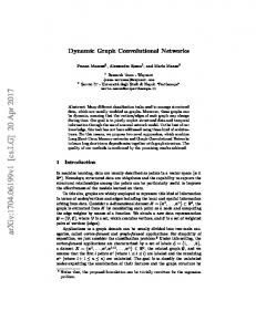
A Capsule Vector (for example containing moments)   P a0k xk (mean) k   P  a0k (xk − µ)2 (std.)    1  Pk [xℓ=1 xk −µ 3 0 ]=  ) (skewness) a ( |N0 |  0k  σ   k .. .

[x1 ]

2

0

1

Figure 1. Above figure shows that the graph capsule function at node 0 computes a capsule vector which encodes higherorder statistical information about its local neighboorhood (per feature). Here {x0 , x1 , x2 , x3 } are respective node feature values. For example, when a node has no more than two neighbors then it is possible to recover back the input node neighbors values from the very first three statistical moments.



 W1 !    W2  f (X, L) = σ X LX . . . Lk X  .  | {z }  ..  g(X,L) Wk (1) | {z } learning weight parameters

=σ

K X k=0

Lk XWk

In Equation 1, g(X, L) ∈ RN ×kd is defined as a graph convolution filter of polynomial form with degree k. While [W1 , W2 , ..., Wk ] are learning weight parameters where each Wk ∈ Rd×h . Note that the g(X, L) = [X, LX, ..., LK X] ∈ RN ×kd can be seen as a new node feature matrix with extended dimension kd 1 . Furthermore, L can be replaced by any other suitable filter matrix as mentioned in (Levie et al., 2017; Kipf & Welling, 2016). A GCNN model with a depth of ℓ−layers can recursively be written as, (2) f (ℓ) (X, L) = σ g(f (ℓ−1) (X, L), L)W(ℓ) where Wℓ ∈ Rkd×h is the weight parameter in ℓth −layer. One can notice that in any layer the basic computation expression involve is [Lk f (ℓ−1) (X, L)]ij . This expression represents that the new j th feature value of ith node (associated with the ith row) is yielded out as a single (scalar) aggregated value based on its local-hood neighbors. This 1

Also referred as the breadth of a GCNN layer .

particular operation can incur significant loss of information. We aim to remedy this issue by introducing our novel GCAPS-CNN model based on the fundamental capsule idea. 3.1. Graph Capsule Networks The core idea behind graph capsule network is to capture more information in local pool beyond aggregation (which is the graph convolution operation in our case). This new information is encapsulated in so called instantiation parameters described in (Hinton et al., 2011) which forms a capsule vector of highly informative outputs. The quality of these parameters are determine by their ability to encode as well decode (i.e., to reconstruct) a node local-hood neighbors feature values from the capsule vector. For instance, one can take the histogram of neighborhood feature values as the capsule vector. If histogram bindwidth is sufficiently small, we can guarantee to recover back all the original input node values. This strategy has widely been used in constructing a successful graph kernel. However, histogram is not a continuous differentiable function and hence cannot employed in end-to-end deep learning. Beside seeking representative instantiation parameters, we further impose two more constraints on a graph capsule function. First, we want our graph capsule function to be permutation invariant (unlike equivariant as discussed in (Hinton et al., 2011)) with respect to input node values since we are interested in a model that can produce the same output for isomorphic graphs. Second, we would like to compute these parameters in fast manner. Graph Capsule Function: To describe a general graph capsule function consider an ith node with x0 value


and set of its neighborhood node values as N (i) = {x0 , x1 , x2 , ..., xk } including itself. In a graph convolution operation output is a scalar function f : Rk → R which takes k input neighbors at ith node and yields output as,

fi (x0 , x1 , ..., xk ) =

X 1 aik xk |N (i)|

(3)

as instantiation parameters because they are permutationally invariant and can nicely be computed through matrixmultiplication operations in a fast manner. To see exactly how, let fp (X, L) be the output matrix corresponding to (ℓ) pth dimension. Then, we can compute fp (X, L) containing statistical moments as instantiation parameters as follows,

k∈N (i)

where aik represents edge weights between nodes i and k. But in graph capsule network, we propose to replace f (x0 , ..., xk ) with a vector value capsule function f : Rk → Rp . For example, consider a capsule function that captures higher-order statistical moments as follows (for simplicity we omit mean and standard deviation),  P  aik xk N (i) k∈P   aik x2k    1 k∈N (i)  fi (x0 , ..., xk ) = (4)   ..  |N (i)|    .  P  aik xck

fp(ℓ) (X, L) K X (ℓ) (ℓ−1) (ℓ−1) =σ Lk (fF (X, L) ⊙ ... ⊙ fF (X, L))Wpk {z } | k=0 p times

(5)

where ⊙ is a hadamard product. Here to keep the feature dimensions in check from growing, we flatten the last two (ℓ−1) dimension of the input as fF lat (X, L) ∈ RN ×hℓ−1 p and performs usual graph convolution operation followed by a (ℓ) linear transformation with Wpk ∈ Rhℓ−1 p×hℓ as the learning weight parameter. Note that here p is used to denote both the capsule dimension as well the order of statistical moments.

k∈N (i)

Figure 1 shows an instance of applying our graph capsule function on a specific node. As a result for an input feature matrix X ∈ RN ×d , our graph capsule network will produce an output f (X, L) ∈ RN ×h×p where p is the number of instantiation parameters.

Graph Capsule Function with Polynomial Coefficients: As mentioned earlier, the quality of instantiation parameters depend upon their capability to encode and decode the input values. Therefore, we seek capsule functions which are bijective in nature i.e., guaranteed to preserve everything about the local neighborhood. For instance, one consider coefficients of polynomial as instantiation parameters by taking the set of local node feature values as roots,

Managing Graph Capsule Vector Dimension: In the first layer, our graph capsule network receives an input X ∈ RN ×d and produces a non-linear output f (1) (X, L) ∈ RN ×h1 ×p . Since our graph capsule function produces a vector of p dimension (for each input d dimension), the feature dimension of the output in subsequent layers can quickly blow up to an unmanageable value. To keep it check, we restrict the feature dimension of the output f (ℓ) (X, L) to be always ∈ RN ×hℓ ×p at any middle ℓth −layer of GCAPS-CNN (here hℓ represents the hidden dimension of that layer). This can be accomplished in two ways 1) either by flattening the last two dimension of f (X, L) and carrying out graph convolution in usual way (see Equation 5 for an example) 2) or by taking the weighted combination of p−dimension capsule vectors (this is similar to performing attention mechanism) at each node as performed in (Sabour et al., 2017). We leave the second approach for our future work. Thus in a nutshell, our graph capsule network in ℓth −layer (ℓ > 1) receives an input f (ℓ−1) (X, L) ∈ RN ×hℓ−1 ×p and produces an output f (ℓ) (X, L) ∈ RN ×hℓ ×p .

One can show that from a given full set of polynomial coefficients, we are guaranteed to recover back all the original node values (upto permutation). However, the first issue with this approach is that they are expensive to compute at each node. Specifically, a combinatorial algorithm without fast fourier transform takes O (k 2 ) complexity to compute where k is the number of roots. Also, there is numerical instability issue associated with computing polynomial coefficients. There are ways to deal with these kind issues but we leave pursuing this direction for our future work.

Graph Capsule Function with Statistical Moments: In this paper, we consider higher-order statistical moments

In short, our graph capsule idea is powerful and can be employed in any type of GCNN model for either solving graph



P

xk



k∈N (i)   P  xk1 xk2     ,k2 ∈N (i) 1    k1P fi (·) =  xk1 xk2 xk3   |N (i)| k1 ,k2 ,k3 ∈N (i)     . ..   x0 x1 xk−1 xk

(6)


semi-supervised learning problem or performing sequence learning on graphs using Graph Recurrent Neural Network models (GCRNNs) or doing link prediction via Graph Autoencoders (GAEs) or/and for generating synthetic graphs through Graph Generative Adversarial models (GGANs).

4. Designing Graph Permutation Invariant Layer In this section, we focus on the second limitation of GCNN model regarding achieving permutation invariance for graph classification purpose. Before presenting our novel invariant layer in GCAPS-CNN model, we first discuss the shortcomings of Max-Sort Pooling Layer which is the next popular choice after aggregation for achieving invariance. 4.1. Problems with Max-Sort Pooling Layer We design a test to determine whether the invariant graph feature constructed by a model has any degree of certainty to produce the same output for sub-graph isomers or not. Sub-Graph Isomorphism Feature Test: Consider two graphs G1 = (V1 , E1 ) and G2 = (V2 , E2 ) such that G1 is isomorphic to a sub-graph of G2 . Let f1 , f2 ∈ Rk be the invariant feature vector (w.r.t. to graph isomorphism) of G1 , G2 respectively. Then, we define sub-graph isomorphism feature test as a criteria providing guarantee that each elements of f1 and f2 are comparable under certain notion i.e., f1i ≡ f2i for any i ∈ [1, k]. Here ≡ represents a comparison operator defined in a sensible way. Satisfying this test is very desirable for graph classification problem since it is quite likely that sub-graph isomers of a graph belong to the same class label. This property helps the model to learn wi weight parameter appropriately which is shared across the same input place i.e., f1i and f2i . Proposition 1 Let f1 , f2 ∈ Rk be the feature vectors containing top k − max node values in sorted order for graphs G1 , G2 respectively and given G1 is sub-graph isomorphic to G2 . Then the Max-Sort Pooling Layer fails the Subgraph Isomorphism Feature Test owing to the comparison done with respect to node ordering. Remarks: Max-Sort Pooling layer fails the test because it does not guarantee that f1i 6≡ f2i for any i ∈ [1, k]. Here 6≡ (not comparable) operator represents that the node corresponding to values f1i and f2i may not be the same in sub-graph isomers. Even including a single node (value) in f2 vector which is not present in G1 can mess up the whole comparision order of f1 and f2 elements. As a result, in Max-Sort Pooling layer the comparison is not always guaranteed to be sensible which makes the problem of learning weight parameters harder. In general, any invariant graph

feature vector that relies on node ordering will fail this test. 4.2. Covariance as Permutation Invariant Layer Our novel idea of permutation invariant features in GCAPSCNN model is computing the covariance of f (X, L) layer output given as follows,

C (f (X, L)) =

1 (f (X, L) − µ)T (f (X, L) − µ) N

(7)

Here µ is the mean of f (X, L) output and C (·) is a covariance function. Since covariance function is differentiable and does not depends upon the order of row elements, it can serve as a permutation invariant layer in GCAPSCNN model. Also, it is fast in computation due to a single matrix-multiplication operation. Note that we flatten the last two dimension of GCAPS-CNN layer output f (X, L) ∈ RN ×h×p in order to compute the covariance. Moreover, covariance provides much richer information about the data by including shapes, norms and angles (between node hidden features) information rather than just providing the mean of data. Infact in multivariate normal distribution, it is used as a statistical parameter to approximate the normal density and thus also reflects information about the data distribution. This particular property along with invariance has been exploited before in (Kondor & Jebara, 2003) for computing similarity between two set of vectors. One can also think about fitting multivariate normal distribution on f (X, L) but it involves computing inverse of covariance matrix which is computationally expensive. Since each element of covariance matrix is invariant to node orders, we can flatten the symmetric covariance matrix C ∈ Rhp×hp to construct the graph invariant feature vector f ∈ R(hp+1)hp/2 . On an another positive note, here the output dimension of f does not depend upon N number of nodes and can be adjusted according to computational constraints. Proposition 2 Let f1 , f2 ∈ Rk be the feature vectors containing covariance elements of node feature matrices for graphs G1 , G2 respectively and given G1 is sub-graph isomorphic to G2 . Then the covariance invariant layer pass the Sub-Graph Isomorphism Feature Test owing to the comparison done with respect to feature dimensions. Remarks: It is quite straightforward to see that the feature dimension order of a node does not depend upon the graph node ordering and hence the order is same across all graphs. As a result, each elements of f1 and f2 are always comparable. To be more specific, covariance output compares both the norms sand angles between the corresponding pairs of feature dimension vectors in two graphs.


5. Designing GCAP-CNN with Global Features Besides guaranteeing permutation invariance in GCAPCNN model, another important desired characteristic of graph classification model is to capture global structure (or features) of a graph. For instance, considering only node degree (as a node feature) is a local information and not much helpful towards solving graph classification problem. On the other hand, considering spectral embedding as a node feature takes global piece of information into account and have been proven successful in serving as a node vector for problems dealing with graph semi-supervised learning. We define global features that takes full graph structure into account during their computation. While local features only depend upon some (at-most) k−hop node neighbors . Unfortunately, the basic design of GCNN model can only capture local structure information of the graph at each node. We make this loose statement more concrete with the following theorem. Theorem 1 : Let G be a graph with L ∈ RN ×N graph Laplacian and X ∈ RN ×d node feature matrix. Let f (ℓ) (X, L) be the output function of a ℓth GCNN layer equipped with polynomial filters of degree k. Then [f (ℓ) (X, L)]i output at ith node (i.e., ith row in f (ℓ) (·)) depends upon “only” on the input values of neighbors distant at most “kℓ−hops” away. Proof: We can proof this statement by mathematical induction. It is easy to see that the base case ℓ = 1 holds true. Lets assume it also holds true for f (ℓ−1) (X, L) i.e., ith node output depends upon neighbors distant upto away. Then in f (ℓ) (X, L) = k × (ℓ − 1) hop σ g f (ℓ−1) (X, L), L W(ℓ) we focus on the term, g(X, L) = [f (ℓ−1) (X, L), . . . , Lk f (ℓ−1) (X, L)]

(8)

particularly the last term involving Lk f (ℓ−1) (X, L). Matrix multiplication of Lk with f (ℓ−1) (X, L) will result in ith node to include all node information which are at-most k−hop distance away. But since a node in f (ℓ−1) (X, L) at a distance k−hops (from ith node) can contain information upto k × (ℓ − 1) hops, we have ith node containing information at-most k + k(ℓ − 1) = kℓ hops distance away. Remarks: Above theorem 1 establishes that GCNN model with ℓ layers can capture only kℓ−hop local-hood structure information at each node. Thus, employing GCNN for graph classification with say aggregation layer can capture only average variation of kℓ−hop local-hood information over the whole graph. To include more global information about the graph one can either increase k (i.e, choose

higher order graph convolution filters) or ℓ (i.e, the depth of GCNN model). Both these choices increases model complexity and thus would require more data samples to reach satisfying results. However among the two, we prefer increasing the depth of GCNN model because the first choice leads to increase in the breadth of the GCNN layer (see footnote 1 about g(X, L) in Section 3) and based on the current understanding of deep learning theory, increasing the depth is favored more over the breadth. For cases where graph node features are missing, it is a common practice to take node degree as a node feature. Such practices can work for problems like graph semisupervised where local-structure information drives node output labels (or classes). But in graph classification global features governs the output labels and hence taking node degree is not sufficient. Of course, we can go for a very deep GCNN model that will allows us to exploit more global information but requires higher sample complexity to achieve satisfying results. To balance the two (model complexity with depth vs. required sample complexity), we propose to incorporate F GSD features in our GCAP-CNN model computed at each node. As shown in (Verma & Zhang, 2017) F GSD features capture global information about the graph and can also be computed in fast manner. Specifically, at each ith node F GSD features are computed as the histogram of the multiset formed by taking the harmonic distance between all nodes and the ith node. It is given by,

S (x, y) =

N −1 X n=0

1 (φn (x) − φn (y))2 λn

(9)

where S (x, y) is the harmonic distance, x, y are any graph nodes and λn , φn (·) is the nth eigenvalue and eigenvector respectively. In our experiments, we employ these features only for datasets where node feature are missing (specifically for social network datasets in our case). Although this strategy can always be used by concatenating F GSD features with original node feature values to capture more global information. Further inspired from Weisfeiler-lehman graph kernel (Shervashidze et al., 2011) which also concatenate features in each labeling iteration, we also propose to pass concatenated outputs from intermediate layers to our covariance and fully connected layers. Finally, our whole end-to-end GCAP-CNN learning model is guaranteed to produce the same output for isomorphic graphs.

6. Experiment and Results GCAPS-CNN Model Configuration: We build ℓ layer GCAPS-CNN with following configuration: Input →

Graph Capsule Convolutional Neural Networks Dataset

PTC

PROTEINS

NCI1

NCI109

D&D

ENZYMES

(No. Graphs)

344

1113

4110

4127

1178

600

(Max. Graph Size)

109

620

111

111

5748

126

(Avg. Graph Size)

25.56

39.06

29.80

29.60

284.32

32.60

Deep Learning Methods DCNN[2016]

56.60 ± 2.89

61.29 ± 1.60

56.61 ± 1.04

57.47 ± 1.22

58.09 ± 0.53

42.44 ± 1.76

PSCN[2016]

62.29 ± 5.68

75.00 ± 2.51

76.34 ± 1.68

—

—

—

ECC[2017]

—

—

76.82

75.03

72.54

45.67

DGCNN[2018]

58.59 ± 2.47

75.54 ± 0.94

74.44 ± 0.47

75.03 ± 1.72

79.37 ± 0.94

51.00 ± 7.29

GCAPS-CNN

66.01 ± 5.91

76.40 ± 4.17

82.72 ± 2.38

81.12 ± 1.28

77.62 ± 4.99

61.83 ± 5.39

Graph Kernels RW[2003]

57.85 ± 1.30

74.22 ± 0.42

> 1 Day

> 1 Day

> 1 Day

24.16 ± 1.64

SP[2005]

58.24 ± 2.44

75.07 ± 0.54

73.00 ± 0.24

73.00 ± 0.21

> 1Day

40.10 ± 1.50

GK[2009]

57.26 ± 1.41

71.67 ± 0.55

62.28 ± 0.29

62.60 ± 0.19

78.45 ± 1.11

26.61 ± 0.99

WL [2011]

57.97 ± 0.49

74.68 ± 0.49

82.19 ± 0.18

82.46 ± 0.24

79.78 ± 0.36

52.22 ± 1.26

DGK[2015]

60.08 ± 2.55

75.68 ± 0.54

80.31 ± 0.46

80.32 ± 0.33

73.50 ± 1.01

53.43 ± 0.91

MLG[2016]

63.26 ± 1.48

76.34 ± 0.72

81.75 ± 0.24

81.31 ± 0.22

78.18 ± 2.56

61.81 ± 0.99

GCAPS-CNN

66.01 ± 5.91

76.40 ± 4.17

82.72 ± 2.38

81.12 ± 1.28

77.62 ± 4.99

61.83 ± 5.39

Table 1. Classification accuracy on bioinformatics datasets. Result in bold indicates the best reported classification accuracy. Top half of the table compares results with various deep learning approaches while bottom half compares results with graph kernels. ‘> 1 day’ represents that the computation exceed more than 24hrs. ‘OMR’ is out of memory error. GC(h, p) → · · · → GC(h, p) → [M, C(·)] → F C(h) → F C(h) → Sof tmax. Here GC(h, p) represents a Graph Capsule CNN layer with h hidden dimensions and p instantiation parameters. As mentioned earlier, we take the intermediate output of each GC(h, p) layers and form a concatenated tensor which is subsequently pass through [M, C(·)] layer which computes mean and covariance of the input. Output of [M, C(·)] layer is then passed to two fully connected F C layers with again h output dimensions and finally connects to a softmax layer for computing class probabilities. In between intermediate layers, we use batch normalization and dropout technique to prevent overfitting along with L2 norm regularization. We set ℓ ∈ {2, 3, 4} depending upon the dataset size (towards higher for larger dataset) and h ∈ {32, 64, 128} for setting hidden dimension. We restrict p ∈ [1, 4] for computing higher-order statistical moments due to computational constraints. Further, we employ ADAM optimization technique with initial learning rate chosen from the set {10−1, . . . , 10−7 } with a decaying factor of 0.1 after every few epochs. Batch size is set according to the given dataset size and memory requirements. Number of epochs are chosen from the set {100, 200, 500, 1000}. All the above mentioned hyper-

parameters are tuned based on the training loss. Average classification accuracy based on 10−fold cross validation error is reported for each dataset. Our GCAPS-CNN code and data will be made available at Github2 . Datasets: To evaluate our GCAPS-CNN model, we perform graph classification tasks on variety of benchmark datasets. In first round, we used 6 bioinformatics datasets namely: PTC, PROTEINS, NCI1, NCI109, D&D, and ENZYMES. In second round, we used 5 social network datasets namely: COLLAB, IMDB-BINARY, IMDB-MULTI, REDDIT-BINARY and REDDIT-MULTI5K. D&D dataset contains 691 enzymes and 587 nonenzymes proteins structures. For other datasets details can be found in (Yanardag & Vishwanathan, 2015). Also for each dataset number of graphs, maximum and average number of nodes is shown in the Table 1 and Table 2. Experimental Set-up: All experiments were performed on a single machine loaded with recently launched 2×NVIDIA TITAN VOLTA GPUs and 64 GB RAM. We compare our method with both deep learning models and 2

https://github.com/vermaMachineLearning/Graph-CapsuleCNN-Networks/

Graph Capsule Convolutional Neural Networks Dataset

COLLAB

IMDB-BINARY

IMDB-MULTI

REDDIT-BINARY

REDDIT-MULTI

(No. Graphs)

5000

1000

1500

2000

5000

(Max. Graph Size)

492

136

89

3783

3783

(Avg. Graph Size)

74.49

19.77

13.00

429.61

508.5

Deep Learning Methods DCNN[2016]

52.11 ± 0.71

49.06 ± 1.37

33.49 ± 1.42

OMR

OMR

PSCN[2016]

72.60 ± 2.15

71.00 ± 2.29

45.23 ± 2.84

86.30 ± 1.58

49.10 ± 0.70

DGCNN[2018]

73.76 ± 0.49

70.03 ± 0.86

47.83 ± 0.85

76.02 ± 1.73

48.70 ± 4.54

GCAPS-CNN

77.71 ± 2.51

71.69 ± 3.40

48.50 ± 4.10

87.61 ± 2.51

50.10 ± 1.72

Graph Kernels GK[2009]

72.84 ± 0.28

65.87 ± 0.98

43.89 ± 0.38

77.34 ± 0.18

41.01 ± 0.17

DGK[2015]

73.09 ± 0.25

66.96 ± 0.56

44.55 ± 0.52

78.04 ± 0.39

41.27 ± 0.18

GCAPS-CNN

77.71 ± 2.51

71.69 ± 3.40

48.50 ± 4.10

87.61 ± 2.51

50.10 ± 1.72

Table 2. Classification accuracy on social network datasets. Result in bold indicates the best reported classification accuracy. Top half of the table compares results with various deep learning approaches while bottom half compares results with graph kernels. ‘> 1 day’ represents that the computation exceed more than 24hrs. ‘OMR’ is out of memory error. graph kernels. Deep Learning Baselines: For deep learning approaches, we adopted 4 recently proposed state-of-art graph convolutional neural networks namely: PATCHYSAN (PSCN) (Niepert et al., 2016), Diffusion CNNs (DCNN) [(Atwood & Towsley, 2016)], Dynamic Edge CNN (ECC) (Simonovsky & Komodakis, 2017) and Deep Graph CNN (DGCNN) (Zhang et al., 2018). Graph Kernel Baselines: We adopted 6 state-ofart graphs kernels for comparison namely: Random Walk (RW) (Gärtner et al., 2003), Shortest Path Kernel (SP) (Borgwardt & Kriegel, 2005), Graphlet Kernel (GK) (Shervashidze et al., 2009), Weisfeiler-Lehman Sub-tree Kernel (WL) (Shervashidze et al., 2011), Deep Graph Kernels (DGK) (Yanardag & Vishwanathan, 2015) and Multiscale Laplacian Graph Kernels (MLK) (Kondor & Pan, 2016). Baselines Settings: We adopted the same procedure from previous works (Niepert et al., 2016; Yanardag & Vishwanathan, 2015; Zhang et al., 2018) to make a fair comparison and used 10-fold cross validation with LIBSVM (Chang & Lin, 2011) library to report the classification performance for graph kernels. Parameters of SVM are independently tuned using training folds data and best average classification accuracies are reported for each method. For Random-Walk (RW) kernel, decay factor is chosen from {10−6, 10−5 ..., 10−1 }. For Weisfeiler-Lehman (WL) kernel, we chose height of subtree kernel from h ∈ {2, 3, 4}. For graphlet kernel

(GK), we chose graphlets size {3, 5, 7} and for deep graph kernels (DGK), we report the best classification accuracy obtained among: deep graphlet kernel, deep shortest path kernel and deep Weisfeiler-Lehman kernel. For Multiscale Laplacian Graph (MLG) kernel, we chose η and γ parameter of the algorithm from {0.01, 0.1, 1}, radius size from {1, 2, 3, 4}, and level number from {1, 2, 3, 4}. For diffusion-convolutional neural networks (DCNN), we chose number of hops from {2, 5}. For the rest, best reported results were borrowed from papers PATCHY-SAN (k = 10) (Niepert et al., 2016), ECC (Simonovsky & Komodakis, 2017) (without edge labels since all other methods also relies on only node labels) and DGCNN (with sorting layer) (Zhang et al., 2018), since the experimental setup was the same and a fair comparison can be made. In short, we follow the same procedure as mentioned in previous papers. Note: some results are not present because either they are not previously reported or source code not available to run them. Graph Classification Results: From Table 1, it is clear that our GCAPS-CNN model consistently outperforms most of the considered deep learning methods on bioinformatics datasets (except on D&D dataset) with a significant margin of 1% − 6% classification accuracy gain (highest being on NCI1 dataset). Again, this trend is continued to be the same on social network datasets as shown in Table 2. Here, we were able to achieve upto 4% accuracy gain on COLLAB dataset and


rest were around 1% gain with consistency when compared against other deep learning approaches. Our GCAPS-CNN is also very competitive with state-ofart graph kernel methods. It again show a consistent performance gain of 1% − 3% accuracy (highest being on PTC dataset) on many bioinformatic datasets when compared against with strong graph kernels. While other considered deep learning methods are not even close enough to beat graph kernels on many of these datasets. It is worth mentioning that the most deep learning models (like ours) are also scalable while graph kernels are more fine tuned towards handling small graphs. For social network datasets, we have a significant gain of atleast 4% − 9% accuracy (highest being on REDDITMULTI dataset) against graph kernels as observed in Table 2. But this is expected as deep learning methods tend to do better with the large amount of data available for training on social networks datasets. Altogether, our GCAPSCNN model shows very promising results against both the current state-of-art deep learning methods and graph kernels.

7. Conclusion & Future Work In this paper, we present a novel Graph Capsule Network (GCAPS-CNN) model based on the fundamental capsule idea to address some of the basic weaknesses of existing GCNN models. Our graph capsule network model by design captures more local structure information than traditional GCNN and can provide much richer representation of individual graph nodes or for the whole graph. For our purpose, we employ a capsule function that preserves statistical moments formation since they are faster to compute. Furthermore, we propose a novel permutation invariant layer based on computing covariance in our GCAPSCNN architecture to deal with graph classification problem which most GCNN models find challenging. This covariance can again be computed in a fast manner and has shown to be better than adopting aggregation or max-sort pooling layer. On the top, we also propose to equip our GCAPS-CNN model with F GSD features explicitly to capture more global information in absence of node features. This is essential to consider since non-deep GCNN models are not capable enough to exploit global information implicitly. Finally, we show GCAPS-CNN superior performance on many bioinformatics and social network datasets in comparison with existing deep learning methods as well as strong graph kernels and set the current state-of-the-art. Our general idea of graph capsule is quite rich and can taken to another level by designing more sophisticated capsule functions that are capable of preserving more information in a local pool. In our future work, we will investigate

various other capsule functions such as polynomial coefficients (as instantiation parameters) which comes with theoretical guarantees. Another choice, we will investigate is performing kernel density estimation technique in end-toend deep learning framework and understanding their theoretical significance. Lastly, we will also explore the other approach of managing the graph capsule vector dimension as discussed in (Sabour et al., 2017).

References Atwood, James and Towsley, Don. Diffusion-convolutional neural networks. In Advances in Neural Information Processing Systems, pp. 1993–2001, 2016. Borgwardt, Karsten M and Kriegel, Hans-Peter. Shortestpath kernels on graphs. In Data Mining, Fifth IEEE International Conference on, pp. 8–pp. IEEE, 2005. Bruna, Joan, Zaremba, Wojciech, Szlam, Arthur, and LeCun, Yann. Spectral networks and locally connected networks on graphs. arXiv preprint arXiv:1312.6203, 2013. Chang, Chih-Chung and Lin, Chih-Jen. Libsvm: a library for support vector machines. ACM Transactions on Intelligent Systems and Technology (TIST), 2(3):27, 2011. Dai, Hanjun, Dai, Bo, and Song, Le. Discriminative embeddings of latent variable models for structured data. In International Conference on Machine Learning, pp. 2702–2711, 2016. de Vries, Gerben KD. A fast approximation of the weisfeiler-lehman graph kernel for rdf data. In Joint European Conference on Machine Learning and Knowledge Discovery in Databases, pp. 606–621. Springer, 2013. Defferrard, Michaël, Bresson, Xavier, and Vandergheynst, Pierre. Convolutional neural networks on graphs with fast localized spectral filtering. In Advances in Neural Information Processing Systems, pp. 3837–3845, 2016. Duvenaud, David K, Maclaurin, Dougal, Iparraguirre, Jorge, Bombarell, Rafael, Hirzel, Timothy, AspuruGuzik, Alán, and Adams, Ryan P. Convolutional networks on graphs for learning molecular fingerprints. In Advances in neural information processing systems, pp. 2224–2232, 2015. Feragen, Aasa, Kasenburg, Niklas, Petersen, Jens, de Bruijne, Marleen, and Borgwardt, Karsten. Scalable kernels for graphs with continuous attributes. In Advances in Neural Information Processing Systems, pp. 216–224, 2013.


Garc´ıa-Durán, Alberto and Niepert, Mathias. Learning graph representations with embedding propagation. arXiv preprint arXiv:1710.03059, 2017.

Lei, Tao, Jin, Wengong, Barzilay, Regina, and Jaakkola, Tommi. Deriving neural architectures from sequence and graph kernels. arXiv preprint arXiv:1705.09037, 2017.

Gärtner, Thomas, Flach, Peter, and Wrobel, Stefan. On graph kernels: Hardness results and efficient alternatives. In Learning Theory and Kernel Machines, pp. 129–143. Springer, 2003.

Levie, Ron, Monti, Federico, Bresson, Xavier, and Bronstein, Michael M. Cayleynets: Graph convolutional neural networks with complex rational spectral filters. arXiv preprint arXiv:1705.07664, 2017.

Gilmer, Justin, Schoenholz, Samuel S, Riley, Patrick F, Vinyals, Oriol, and Dahl, George E. Neural message passing for quantum chemistry. arXiv preprint arXiv:1704.01212, 2017.

Montavon, Grégoire, Hansen, Katja, Fazli, Siamac, Rupp, Matthias, Biegler, Franziska, Ziehe, Andreas, Tkatchenko, Alexandre, Lilienfeld, Anatole V, and Müller, Klaus-Robert. Learning invariant representations of molecules for atomization energy prediction. In Advances in Neural Information Processing Systems, pp. 440–448, 2012.

Henaff, Mikael, Bruna, Joan, and LeCun, Yann. Deep convolutional networks on graph-structured data. arXiv preprint arXiv:1506.05163, 2015. Hinton, Geoffrey E, Krizhevsky, Alex, and Wang, Sida D. Transforming auto-encoders. In International Conference on Artificial Neural Networks, pp. 44–51. Springer, 2011. Kashima, Hisashi, Tsuda, Koji, and Inokuchi, Akihiro. Marginalized kernels between labeled graphs. In ICML, volume 3, pp. 321–328, 2003. Kipf, Thomas N and Welling, Max. Semi-supervised classification with graph convolutional networks. arXiv preprint arXiv:1609.02907, 2016. Kondor, Risi and Borgwardt, Karsten M. The skew spectrum of graphs. In Proceedings of the 25th international conference on Machine learning, pp. 496–503. ACM, 2008. Kondor, Risi and Jebara, Tony. A kernel between sets of vectors. In Proceedings of the 20th International Conference on Machine Learning (ICML-03), pp. 361–368, 2003. Kondor, Risi and Pan, Horace. The multiscale laplacian graph kernel. In Advances in Neural Information Processing Systems, pp. 2982–2990, 2016. Kondor, Risi, Shervashidze, Nino, and Borgwardt, Karsten M. The graphlet spectrum. In Proceedings of the 26th Annual International Conference on Machine Learning, pp. 529–536. ACM, 2009. Kondor, Risi, Son, Hy Truong, Pan, Horace, Anderson, Brandon, and Trivedi, Shubhendu. Covariant compositional networks for learning graphs. arXiv preprint arXiv:1801.02144, 2018. Kriege, Nils M, Giscard, Pierre-Louis, and Wilson, Richard. On valid optimal assignment kernels and applications to graph classification. In Advances in Neural Information Processing Systems, pp. 1623–1631, 2016.

Neumann, Marion, Patricia, Novi, Garnett, Roman, and Kersting, Kristian. Efficient graph kernels by randomization. In Joint European Conference on Machine Learning and Knowledge Discovery in Databases, pp. 378– 393. Springer, 2012. Niepert, Mathias, Ahmed, Mohamed, and Kutzkov, Konstantin. Learning convolutional neural networks for graphs. In Proceedings of the 33rd annual international conference on machine learning. ACM, 2016. Orsini, Francesco, Frasconi, Paolo, and De Raedt, Luc. Graph invariant kernels. In IJCAI, pp. 3756–3762, 2015. Prˇzulj, Nataˇsa. Biological network comparison using graphlet degree distribution. Bioinformatics, 23(2): e177–e183, 2007. Sabour, Sara, Frosst, Nicholas, and Hinton, Geoffrey E. Dynamic routing between capsules. In Advances in Neural Information Processing Systems, pp. 3859–3869, 2017. Shervashidze, Nino, Vishwanathan, SVN, Petri, Tobias, Mehlhorn, Kurt, and Borgwardt, Karsten M. Efficient graphlet kernels for large graph comparison. In AISTATS, volume 5, pp. 488–495, 2009. Shervashidze, Nino, Schweitzer, Pascal, Leeuwen, Erik Jan van, Mehlhorn, Kurt, and Borgwardt, Karsten M. Weisfeiler-lehman graph kernels. Journal of Machine Learning Research, 12(Sep):2539–2561, 2011. Shuman, David I, Narang, Sunil K, Frossard, Pascal, Ortega, Antonio, and Vandergheynst, Pierre. The emerging field of signal processing on graphs: Extending highdimensional data analysis to networks and other irregular domains. IEEE Signal Processing Magazine, 30(3): 83–98, 2013. Simonovsky, Martin and Komodakis, Nikos. Dynamic edge-conditioned filters in convolutional neural networks on graphs. In Proc. CVPR, 2017.


Verma, Saurabh and Zhang, Zhi-Li. Hunt for the unique, stable, sparse and fast feature learning on graphs. In Advances in Neural Information Processing Systems, pp. 87–97, 2017. Yanardag, Pinar and Vishwanathan, SVN. Deep graph kernels. In Proceedings of the 21th ACM SIGKDD International Conference on Knowledge Discovery and Data Mining, pp. 1365–1374. ACM, 2015. Zhang, Muhan, Cui, Zhicheng, Neumann, Marion, and Chen, Yixin. An end-to-end deep learning architecture for graph classification. In AAAI, pp. 4438–4445, 2018. Zhao, Xiaohan, Zong, Bo, Guan, Ziyu, Zhang, Kai, and Zhao, Wei. Substructure assembling network for graph classification. 2018.