standard Slepian-Wolf coding scheme at the Orlitsky-Roche rate. We establish that a minimum (conditional) entropy coloring of the product of characteristic ...
Graph Coloring and Conditional Graph Entropy Vishal Doshi, Devavrat Shah, Muriel M´edard, Sidharth Jaggi Laboratory for Information and Decision Systems Massachusetts Institute of Technology Cambridge, MA 02139 {vdoshi, devavrat, medard, jaggi} @ mit.edu Abstract— We consider the remote computation of a function of two sources where one is receiver side information. Specifically, given side information Y , we wish to compute f (X, Y ) based on information transmitted by X over a noise-less channel. The goal is to characterize the minimal rate at which X must transmit information to enable the computation of the function f . Recently, Orlitsky and Roche (2001) established that the conditional graph entropy of the characteristic graph of the function is a solution to this problem. Their achievability scheme does not separate “functional coding” from the well understood distributed source coding problem. In this paper, we seek a separation between the functional coding and the coding for correlation. In other words, we want to preprocess X (with respect to f ), and then transmit the preprocessed data using a standard Slepian-Wolf coding scheme at the Orlitsky-Roche rate. We establish that a minimum (conditional) entropy coloring of the product of characteristic graphs is asymptotically equal to the conditional graph entropy. This can be seen as a generalization of a result of K¨orner (1973) which shows that the minimum entropy coloring of product graphs is asymptotically equal to the graph entropy. Thus, graph coloring provides a modular technique to achieve coding gains when the receiver is interested in decoding some function of the source.
I. I NTRODUCTION Consider a network of sensors relaying correlated measurements to a central receiver with measurements of its own. Usually, the receiver is interested in computing a function of the received data. Hence, to the receiver the bulk of the data received from the various sensors is irrelevant. Contemporary data compression techniques (see [1], [2]) compress the data utilizing only the correlation of the measurements and do not take the receiver’s function of interest into account. To increase the efficiency for such a system, we seek to implement better compression rates by exploiting the end-user’s intentions (the computation of the function f of the data received). Consider the following example: suppose there is a source (uniformly) producing an n-bit integer. The receiver also produces an n-bit integer and is only interested in the parity of the sum. Assuming independence of the integer data, contemporary techniques would have the source transmit all n bits, when it is clear that only the final bit is necessary. The use of such compression techniques enables possibly large gains over contemporary methods depending upon the complexity of the function. As a first step towards the implementation of methods like this, we consider the case (as in the example) where there is a single source, denoted by the random variable X with support X . The information available at the receiver is denoted by
"%&!&&%'$()%'*'+*,!'-''
X
ENCODER
DECODER
f(X,Y)
Y Fig. 1. X is encoded such that f (X, Y ) is recovered based on the coded information and side information Y .
the random variable Y with support Y. Both X and Y are discrete memoryless sources. The receiver wishes to compute a function f : X × Y → Z, where Z is some finite set. The goal here is to minimize the rate at which X transmits information to the receiver so as to enable computation of f at the receiver. Figure 1 illustrates the question of interest. A. Setup and Related Work This question has been very well studied in different contexts in the literature [3], [4], [5]. Among them, Orlitsky and Roche [5] recently characterized the minimum rate requirement as the conditional graph entropy of the characteristic graph. We introduce the necessary definitions and notation to explain these results as well as formally state our question of interest. Assume that the random variables X and Y have some joint distribution p(x, y). The n-sequence of random variables, denoted by X and Y are such that (X, Y) = {(Xi , Yi )}ni=1 are i.i.d. with each (Xi , Yi ) drawn according to p(x, y). The receiver is interested in computing a function f : X × Y → Z or f : X n × Y n → Z n , its obvious extension. The primary goal is to determine the minimal rate for X to transmit data to the receiver so that the receiver can compute the function f with vanishing probability of error. Wyner and Ziv [6] considered the side information rate distortion problem. Yamamoto [4] extended their rate distortion function to the case of functional compression. Their functions relied on auxilliary random variables. In a sense, this paper makes those variables explicit for the zero distortion case. Further, we describe them in such a way that our scheme builds upon a Slepian-Wolf coding scheme [7] layered with a preprocessing of the source data. Define the characteristic graph of X with respect to Y , f , and p(x, y) is G = (V, E) with V = X and E defined as follows: an edge (x1 , x2 ) ∈ X 2 is in E if there exists a y ∈
!"#$
Y such that p(x1 , y), p(x2 , y) > 0 and f (x1 , y) $= f (x2 , y). Effectively, G is the “confusability graph” from the perspective of the receiver with side information Y . This was first defined by Witsenhausen [8]. The graph entropy of a graph G with some distribution on its vertices was introduced by Korner [3] and is defined as: HG (X) =
min
X∈W ∈Γ(G)
min
X∈W ∈Γ(G) W −X−Y
X
f(X,Y) COLOR
ENCODE
DECODE
LOOKUP
Y
I(W ; X),
where Γ(G) is the set of all independent sets1 of G. Here, X ∈ W means that the joint distribution p(w, x) on Γ(G)×X is such that p(w, x) > 0 implies x ∈ w. To motivate the importance of graph entropy, consider the following: given a function g : X → Z, define deterministic random variable Y on Y = {1} and set f (x, 1) = g(x) for all x ∈ X . Then, the graph entropy HG (X) is the minimal rate required to distinguish functional values of g [8]. Orlitsky and Roche [5] established that the conditional graph entropy, an extension of graph entropy, is the minimum required transmission rate from X to receiver to compute function f (X, Y ) with small probability of error. The conditional graph entropy is defined as HG (X|Y ) =
Distributed Source Coding
I(W ; X|Y ),
A natural extension of this problem is the computation of rate-distortion region. Yamamoto characterized the ratedistortion function for the question posed here by extending the Wyner-Ziv side information result [6]. This was recently built upon by Feng, Effros and Savari [9]. Our work in this paper is closer (in spirit) to the result by K¨orner [3]. In essence, K¨orner showed that achieving the graph entropy is the same as coloring a large graph and sending the colors. Consider the OR-product graph of G, denoted as Gn = (Vn , En ) where Vn = V n = X n and two vertices (x1 , x2 ) are in En if any component (x1i , x2i ) ∈ E. By coloring, we mean standard graph vertex coloring, i.e. a function c : V → N of a graph G = (V, E) such that (x1 , x2 ) ∈ E implies c(x1 ) $= c(x2 ). The entropy of a coloring is given by the induced distribution on colors p(c(x)) = p(c−1 (c(x))) where c−1 (x) = {¯ x : c(¯ x) = c(x)}. Next, we define ε-colorings of any graph G (for any ε > 0). Let A ⊂ X × Y be any subset such that p(A) ≥ 1 − ε. Define pˆ(x, y) = p(x, y) · 1(x,y)∈A (where 1Q is the indicator function for condition Q). While this is not a true probability, our definition of characteristic graph of X with respect to Y , ˆ Note f , and pˆ is valid. Denote this characteristic graph as G. ˆ is a subset of the set of edges of G. that the set of edges of G Finally, we say c is an ε-coloring of G if it is a valid colorings ˆ defined with respect to some high probability set A. of G The chromatic entropy of a graph is χ HG (X) = inf {H(c(X)) : c is an ε-coloring of G} . ε>0
1 A subset of vertices of a graph is an independent set if no two nodes in the subset are adjacent to each other in G.
Fig. 2. Coloring based coding allows separation between functional coding and distributed source coding as shown above.
We define it’s natural extension conditional chromatic entropy as follows: χ HG (X|Y ) = inf {H(c(X)|Y ) : c is an ε-coloring of G} . ε>0
Now, we state the K¨orner’s result [3] as follows: 1 χ H n (X) = HG (X). n G The result requires ε-colorings and not the simple colorings because, as seen in [10], the ratio of the above quantities can be arbitrarily large. The implications of this result are that for large enough n, one can color a high probability subgraph of the product graph Gn to achieve near optimum functional source coding when the function is only of one source. This effectively layers the solution to a problem of graph coloring followed by using standard coding techniques to transmit the color sequence. The Orlitsky and Roche’s solution is an end-to-end solution. That is, it includes functional and distributed source coding. Their achievability scheme involves coding over the space of independent sets. It is a larger class than the space of colors because each coloring gives rise to disjoint independent sets. Like the implication of K¨orner’s result, the coloring will allow for separation between functional coding and distributed source coding. Hence we want a result similar to that of K¨orner’s result so that the problem can be decoupled without losing any coding gains asymptotically. lim
n→∞
B. Our Contribution As the main result of this paper, we show that the minimum conditional entropy coloring of the OR-product graph is asymptotically the same as the conditional chromatic number. Theorem 1: 1 lim H χ n (X|Y) = HG (X|Y ) n→∞ n G This validates the idea of using graph coloring to achieve better compression ratios. The variable W and the distribution on it that achieves HG (X|Y ) is the auxilliary random variable from the Yamamoto result. In the entropy sense, the induced variable, c(X), converges to W . This method thus leads to a natural layering of the problem just as in K¨orner’s case. Figure 2 illustrates the layering. Nevertheless, we need large enough n to achieve rates close to the conditional graph entropy. Consider the following
!"#(
example from [5]. We have X = Y = {1, 2, 3}, p(x, y) = 16 for all x $= y, and f (x, y) = 1 if x > y and 0 otherwise. Then, our graph G has only one edge: (1, 3). Because of uniformity, χ we know HG (X|Y ) = 23 using the coloring c(1) = c(2) = 1 and c(3) = 2. But HG (X|Y ) ≈ 0.54 bits as calculated in [5]. This is worrisome because minimum entropy graph coloring has been shown to be NP–complete [11]. Nevertheless, the problem is layered into two. The second part is that of distributed source coding which is well understood. There exist methods to achieve corner points of the Slepian-Wolf rate region (e.g. [1]), and there exist methods to achieve all other points on the rate region (e.g. [2]). Further, the first part, that of graph coloring, has very rich literature (e.g. [10], [12]) and heuristics exist (e.g. [13]) for this hard problem.
Distributed Source Coding X
f(X,Y) COLOR
ENCODE
DECODE
LOOKUP
ENCODE
Y Fig. 3. We use Slepian-Wolf codes with Y sending at full rate to achieve the corner point Rx = H(c(X)|Y ).
B. Lower bound
II. P ROOF OF M AIN R ESULT We borrow some techniques that are present in K¨orner [3], Orlitsky and Roche [5]. First, we recall some useful known results. Then, we establish the claimed equality in Theorem 1. A. Preliminaries We begin by listing the results that we will use in our proof. Definition 1 (Typicality): We use the notion of ε-strong typicality defined in [14, p. 358]. For any n, and any sequence x of length n, define the empirical frequency of the symbol x in x as |{i : xi = x}| νx (x) = . n Then a sequence x is ε-strongly typical for ε > 0 if for all x ∈ X with p(x) > 0, ε |νx (x) − p(x)| ≤ , |X |
and for all x ∈ X with p(x) = 0, νx (x) = 0. The set of all such ε-strongly typical sequences, called the ε-typical set will be denoted as Tεn (X), or Tεn when the variables are clear from context. A similar definition naturally extends for the case of joint variables. Lemma 1: Suppose (X, Y) is a sequence of n random variables drawn independently and according to the joint distribution p(x, y), which is the marginal of p(w, x, y). Let an n-sequence W be drawn independently according to its marginal, p(w). Suppose the joint distribution p(w, x, y) forms a Markov Chain, W −X −Y (i.e. p(w, x, y) = p(w|x)p(x, y)). Then, for all ε > 0, there is a ε1 = k · ε, where k depends only on the distribution p(w, x, y), such that for sufficiently large n, 1) P [X ∈ / Tεn ] < ε1 , P [Y ∈ / Tεn ] < ε1 , and P [(X, Y) ∈ / n Tε ] < ε 1 , 2) For all x ∈ Tεn , P [(x, W) ∈ Tεn ] ≥ 2−n(I(W ;X)+ε1 ) . 3) For all y ∈ Tεn , P [(y, W) ∈ Tεn ] ≤ 2−n(I(W ;X)−ε1 ) . 4) For all (w, x) ∈ Tεn , P [(w, Y) ∈ Tεn |(x, Y) ∈ Tεn ] ≥ 1 − ε1 . Part 1 follows from Lemma 13.6.1, parts 2 and 3 follow from Lemma 13.6.2, and part 4 follows from Lemma 14.8.1, all from [14].
To prove the lower bound, consider any n and the corresponding OR-product graph Gn . Let the coloring c of Gn be such that χ HG n (X|Y) = H(c(X)). Such a coloring exists because the number of possible colorings for a graph with n vertices is a finite set. Using this coloring, we will show that there is a scheme that requires rate χ 1 n HGn (X|Y) and provides a way to compute the function at receiver with small probability of error. This will establish the χ achievability of rate n1 HG n (X|Y). By Orlitsky and Roche [5], no scheme can achieve rate smaller than HG (X|Y ). Lemma 2: 1 χ lim inf HG n (X|Y) ≥ HG (X|Y ). n→∞ n Proof: Given n > 0, let the coloring c, as above, denote χ one the coloring that achieves HG n (X|Y) for the OR-product n graph G . For every color, σ and y, define g(σ, y) = f (x, y) where x is any element of c−1 (σ) = {x : c(x) = σ} such that p(x, y) > 0. If no such x exists, g is undefined. Suppose x is the information at the source, and y is the information at the receiver. Without loss of generality, presume p(x, y) > 0. Suppose c(x) and y are available at the decoder. Then, we have an error if g(σ, y) $= f (x, y). Suppose x% ∈ X , c(x% ) = c(x), and p(x% , y) > 0. Because x and x% have the same color, we know (x, x% ) ∈ / En , and therefore for all y where p(x, y), p(x% , y) > 0, including ours, we must have f (x, y) = f (x% , y). Because f has the same value for all x% with p(x% , y) > 0, f (x, y) = g(σ, y). Thus, we have shown that the color of X and Y are sufficient to determine the function f (X, Y). The Slepian-Wolf Theorem [7] states that for two sources, X and Y , there exists a sequence of codes with vanishing probability of error as n grows without bound for the rates: R1 ≥ H(X|Y ), R2 ≥ H(Y |X), and R1 + R2 ≥ H(X, Y ). We apply that theorem to the source (c(X), Y). In our case, Y is side information. In other words, R2 ≥ H(Y ). See Figure 3 for an illustration. Thus, we get the following per symbol rates are achievable for an encoding of X where c is any ε-coloring of Gn (with
!"#.
ε > 0).
1 H(c(X)|Y). n χ Thus, the minimal value of R1 is by definition HG n (X|Y). Putting the above discussion together, we obtain the desired result: 1 χ lim inf HG n (X|Y) ≥ HG (X|Y ) n→∞ n R1 ≥
C. Upper Bound Next we show that, indeed, the information needed to recover cn (X) given Y is at most HG (X|Y ). Lemma 3: 1 χ lim inf HG n (X|Y) ≤ HG (X|Y ). n→∞ n Proof: Suppose ε, δ > 0. Suppose n is large enough so that the following holds: (1) Lemma 1 applies with some ε1 < 1, (2) 2−nδ < ε1 , and (3) n > 2 + 2ε31 . Let p(w, x, y) be the distribution that achieves HG (X|Y ) with the Markov chain, W − X − Y . Let marginals be denoted simply as p(w), p(x), p(y). For any integer M , we define an M -system (W1 , . . . , WM )! where each Wi is drawn n independently according to p(w) = i=1 p(wi ). n Declare an error if (x, y) ∈ / Tε . (Thus, we are in fact looking at colorings over Tεn , or ε1 -colorings.) This, by construction, happens with probability less than ε1 . Henceforth assume that (x, y) ∈ Tεn . Declare an error if there is no i such that (Wi , x) ∈ Tεn . The probability for this event is M (a) " / Tεn ∀i] ≤ P [(Wi , x) ∈ / Tεn ] P [(Wi , x) ∈
%M Using these definitions, s(y) = i=1 1i∈S(y) , where we have used the fact that our coloring scheme cˆ is simply an assignment of the indices of the M -system. Thus, we know E[s(Y)] = Similarly, we get z(y) =
≤ 2−M ·2
E[z(Y)] = ≥ =
1Wi ∈Z(y) . Thus,
i=1 M & i=1 M &
P [Wi ∈ Z(Y)] P [Wi ∈ Z(Y) and i ∈ S(Y)] P [i ∈ S(Y)]P [Wi ∈ Z(Y)|i ∈ S(Y)]
We know that if i ∈ S(Y), there is some x such that cˆ(x) = i and (x, Y) ∈ Tεn . For each such x, we must have (by definition of our coloring), (Wi , x) ∈ Tεn . For each such x where (Wi , x) ∈ Tεn , P [Wi ∈ Z(Y)|i ∈ S(Y)] = P [(Wi , Y) ∈ Tεn |(x, Y) ∈ Tεn ] ≥ 1 − ε1 by Lemma 1, part (4). Thus, we have E[z(Y)] ≥ (1 − ε1 )E[s(Y)]. This and Jensen’s inequality imply that E[log s(Y)] ≤ log E[s(Y)] ( ' z(Y) . ≤ log E 1 − ε1 Finally, using a Taylor series expansion, we know log ε2 = 2ε1 + 12 when 0 < ε1 < 1. Thus,
where (a) and (b) follow because the Wi are i.i.d., (c) follows from Lemma 1, part (2), and (d) follows because for α ∈ [0, 1], (1 − α)n ≤ 2−nα . Assuming M > 2n(I(W ;X)+ε1 +δ) ,
E[log s(Y)] ≤ log E[z(Y)] + ε2 ,
because n is large enough. Henceforth, fix an M -system (W1 , . . . , WM ) for some M > 2n(I(W ;X)+ε1 +δ) . Further, assume there is some i such that (Wi , x) ∈ Tεn . For every x, let the smallest (or any) such i be denoted as cˆ(x). Note that cˆ is a valid coloring of the graph Gn . Next, for each y, define the following:
1 1−ε1
≤ (1)
Next, we compute E[z(Y)] =
P [(Wi , x) ∈ / Tεn ∀i] ≤ 2−δn < ε1 ,
s(y) = |S(y)|, z(y) = |Z(y)|.
M &
i=1
−n(I(W ;X)+ε1 )
S(y) = {ˆ c(x) : (x, y) ∈ Tεn }, Z(y) = {Wi : (Wi , y) ∈ Tεn },
i=1
%M
M
= (1 − P [(W, x) ∈ Tεn ]) $M (c) # ≤ 1 − 2−n(I(W ;X)+ε1 ) (d)
P [i ∈ S(Y)].
i=1
i=1
(b)
M &
M & i=1
P [(Wi , Y) ∈ Tεn ]
= M · P [(Wi , Y) ∈ Tεn ] because the Wi are i.i.d. Therefore, E[z(Y)] ≤ M · 2−n(I(W ;Y )−ε1 )
(2)
by Lemma 1, part (3). By the definition of S(y), we know that determining cˆ given Y = y requires at most log s(y) bits. Therefore, we have H(ˆ c(X)|Y) ≤ E[log s(Y)].
!"&'
(3)
Putting it all together, we have (a)
χ c(X)|Y) HG n (X|Y) ≤ H(ˆ (b)
≤ E[log s(Y)]
(c)
≤ log E[z(Y)] + ε2 $ # ≤ log M · 2−n(I(W ;Y )−ε1 ) + ε2 # $ (e) = log 2n(I(W ;X)−I(W ;Y )+2ε1 +δ) + 1 + ε2 (d)
(f )
≤ n(I(W ; X) − I(W ; Y ) + 2ε1 + δ) + 1 + ε2
where (a) follows by definition of the conditional chromatic entropy, (b) follows from inequality (3), (c) follows from inequality (1), (d) follows from inequality (2), (e) follows by setting M = +2n(I(W ;X)+ε1 +δ) ,, and (f) follows because log(α + 1) ≤ log(α) + 1 for α ≥ 1. We know for Markov chains W − X − Y , I(W ; X) − I(W ; Y ) = I(W ; X|Y ).
Thus, for our optimal distribution p(w, x, y), we have χ HG n (X|Y) ≤ n(HG (X|Y ) + 2ε1 + δ) + 1 + ε2 2 Because n > 2 + 2ε31 , 1+ε < ε1 . Thus, n HG (X|Y ) + 3ε1 + δ. Therefore,
lim sup n→∞
χ 1 n HGn (X|Y)
≤
1 χ H n (X|Y) ≤ HG (X|Y ). n G
Combining the lower bound, Lemma 2, and the upper bound, Lemma 3, we have our result: 1 (4) lim H χ n (X|Y) = HG (X|Y ). n→∞ n G III. C ONCLUSION We have validated the idea of graph coloring to achieve all possible rates. As a consequence, it is possible to decouple the side information functional source coding problem into a problem of graph coloring followed by a coding scheme that removed the redundancy between the colors (like SlepianWolf). While the graph coloring problem is shown to be NP–complete, this decoupling allows for the decomposition of a hard problem into one for which many heuristics and
copious literature exist (graph coloring) and one that is solved (distributed source coding). We plan to show that this decoupling is possible in the more general case when Y is a separate source (and not side information). In this case, we will wish to code both X and Y . This will generalize our current results where we assume the rate for Y is H(Y ). Further, we plan to consider a relaxation of the fidelity criterion. We will wish to see if Yamamoto’s rate distortion function can be achieved with graph coloring, as well as considering the case where Y is not side information. Thus, we hope to have a unified solution that will allow for the distributed compression of functions of correlated sources. R EFERENCES [1] S. S. Pradhan and K. Ramchandran, “Distributed source coding using syndromes (DISCUS): design and construction,” IEEE Trans. Inform. Theory, vol. 49, no. 3, pp. 626–643, Mar. 2003. [2] T. P. Coleman, A. H. Lee, M. M´edard, and M. Effros, “Low-complexity approaches to Slepian-Wolf near-lossless distributed data compression,” IEEE Trans. Inform. Theory, vol. 52, no. 8, pp. 3546–3561, Aug. 2006. [3] J. K¨orner, “Coding of an information source having ambiguous alphabet and the entropy of graphs,” 6th Prague Conference on Information Theory, 1973, pp. 411–425. [4] H. Yamamoto, “Wyner-ziv theory for a general function of the correlated sources,” IEEE Trans. Inform. Theory, vol. 28, no. 5, pp. 803–807, Sept. 1982. [5] A. Orlitsky and J. R. Roche, “Coding for computing,” IEEE Trans. Inform. Theory, vol. 47, no. 3, pp. 903–917, Mar. 2001. [6] A. Wyner and J. Ziv, “The rate-distortion function for source coding with side information at the decoder,” IEEE Trans. Inform. Theory, vol. 22, no. 1, pp. 1–10, Jan. 1976. [7] D. Slepian and J. K. Wolf, “Noiseless coding of correlated information sources,” IEEE Trans. Inform. Theory, vol. 19, no. 4, pp. 471–480, July 1973. [8] H. S. Witsenhausen, “The zero-error side information problem and chromatic numbers,” IEEE Trans. Inform. Theory, vol. 22, no. 5, pp. 592–593, Sept. 1976. [9] H. Feng, M. Effros, and S. Savari, “Functional source coding for networks with receiver side information,” Allerton Conference on Communication, Control, and Computing, Sept. 2004. [10] J. Cardinal, S. Fiorini, and G. Joret, “Minimum entropy coloring,” Lecture Notes on Computer Science, ser. International Symposium on Algorithms and Computation, X. Deng and D. Du, Eds., vol. 3827. Springer-Verlag, 2005, pp. 819–828. [11] J. Cardinal, S. Fiorini, and G. V. Assche, “On minimum entropy graph colorings,” ISIT 2004, June–July 2004, p. 43. [12] C. McDiarmid, “Colourings of random graphs,” in Graph Colourings, ser. Pitman Research Notes in Mathematics Series, R. Nelson and R. J. Wilson, Eds. Longman Scientific & Technical, 1990, pp. 79–86. [13] G. Campers, O. Henkes, and J. P. Leclerq, “Graph coloring heuristics: A survey, some new propositions and computational experiences on random and “Leighton’s” graphs,” in Operations research ’87, G. K. Rand, Ed., 1988, pp. 917–932. [14] T. M. Cover and J. A. Thomas, Elements of Information Theory. New York: Wiley, 1991.
!"&"