is a conflict, the algorithm backtracks, i.e. it goes back to the last consistent state by removing the last color assignment. Then it proceeds to an unexplored ...
Graph coloring: the more colors, the better? Tamás Szép and Zoltán Ádám Mann Budapest University of Technology and Economics Department of Computer Science and Information Theory 1117 Budapest, Magyar tudósok körútja 2, Hungary This paper appeared in: Proceedings of the 11th IEEE International Symposium on Computational Intelligence and Informatics, pages 119-124, Budapest (Hungary), 2010
Abstract—In this paper, we investigate the algorithmic complexity of deciding colorability, as a function of the number of available colors. Intuitively, one may assume that the problem’s complexity is highest around the chromatic number of the graph. We give substantial empirical evidence that this intuition is largely true, both for exact and heuristic graph coloring algorithms. We give a rigorous proof that the complexity of a class of exact algorithms is monotonously increasing in the number of available colors in the non-colorable case, and give a counter-example to demonstrate that the analogous claim does not always hold for colorable graphs.
I. I NTRODUCTION
AND PREVIOUS WORK
Graph coloring is a fundamental problem in algorithmic graph theory, with many practical applications, like frequency assignment [1] or register allocation [4]. For solving graph coloring problems, both exact and heuristic algorithms are widely used. Most exact algorithms use some kind of backtracking to perform an exhaustive search of the possible colorings, while at the same time being able to prune large parts of the search space. Variations of this scheme are branch-and-bound, branch-and-cut, and branch-and-price algorithms [14], [15], [17]. Heuristics include greedy algorithms, genetic algorithms, simulated annealing, and tabu search [3], [5], [9]. In the worst case, graph coloring is NP-complete [6], but many problem instances are eays to color. The systematic study of the complexity of different graph coloring problem instances mostly focuses on random graphs [2], [10], [16], [18], [21], [12]. Most previous work in this area focuses on how the number of nodes and the density of the graph (i.e. the average number of neighbors of a vertex) influence the complexity of the coloring problem. In particular, it is known that the average-case complexity of graph coloring is O(1), meaning that increasing the number of vertices does not increase the complexity of the problem above a given bound. It is also known that the complexity of graph coloring as a function of the density of the graph exhibits an easy-hard-easy pattern [11], [7]. Much less is known about the dependence of the problem complexity on the number of available colors, which we denote by k. Intuitively, one may assume that the problem’s complexity is highest when k is around the chromatic number of the graph, denoted by χ(G). In the colorable case, i.e. when k ≥ χ(G), it is intuitively quite clear that increasing the number of available colors will make it easier to find
a proper coloring of the graph. Hence in this region one expects that the complexity decreases monotonously, both for exact and heuristic algorithms. In the uncolorable region, an exact algorithm’s task is to prove that there exists no proper coloring. This becomes easier when k decreases, since the infeasibility of a region of the search space becomes apparent more quickly if the number of colors is smaller. Hence in this regime one expects complexity to be monotonously increasing. It is generally believed that the complexity is maximal when k = χ(G) − 1 [8]. In this paper, we describe our findings from a systematic study about the dependence of the complexity on the number of available colors. We use two state-of-the-art algorithms, as typical representatives of the kinds of algorithms that are widely used to solve graph coloring problems: • A Branch-and-bound algorithm (BB) as a typical exact algorithm • A genetic algorithm (GA) as a typical heuristic We carried out empirical experiments on random graphs as well as on benchmarks from the literature. Our main findings and contributions are as follows: • As expected, the measured complexity is monotonously increasing in k when k < χ(G) and monotonously decreasing when k ≥ χ(G). • We give a rigorous proof that the BB algorithm’s complexity is monotonously increasing in k when k < χ(G). • We give a counter-example showing that the BB algorithm’s complexity is not always decreasing in k when k ≥ χ(G). (Although in practice this is usually the case.) • The maximum complexity is either at k = χ(G) − 1 or k = χ(G). There can be a significant difference between the complexity of these two cases in both directions; the hypothesis that coloring with χ(G) − 1 colors is more difficult than coloring with χ(G) colors does not seem to be justified. II. P RELIMINARIES A. Problem formulation We consider the graph coloring problem as a decision problem. The input consists of a graph G = (V, E) and a number k ∈ Z+ . The vertices of the graph are denoted by v1 , v2 , . . . , vn , the available colors by 1, 2, . . . , k. A coloring assigns a color to each vertex; a partial coloring assigns a
color to some of the vertices. A (partial) coloring is invalid if there is a pair of adjacent vertices with the same color, otherwise it is valid. The task is to decide whether a valid coloring exists. The chromatic number of the graph, denoted by χ(G), is the minimum k such that G is colorable with k colors. The set of neighbours of a given vertex v will be denoted by N (v). A cut is a set of edges X ⊆ E such that G \ X consists of more components than G. The size of a cut is the number of edges forming the cut. B. The BB algorithm Most of our results relate to the BB algorithm. This is the implementation of the usual backtracking scheme for constraint satisfaction problems, with both generic and problemspecific improvements suggested in the literature. The algorithm assigns colors to the vertices, one at a time, as long as no conflict occurs. If all vertices can be colored this way, the algorithm terminates. On the other hand, when there is a conflict, the algorithm backtracks, i.e. it goes back to the last consistent state by removing the last color assignment. Then it proceeds to an unexplored branch by trying a new color assignment for the currently selected vertex. When all possible branches from a given state have been tried without success, the algorithm backtracks. The algorithm traverses the space of partial solutions in a tree structure. There are two possible termination situations: either a solution is found, or the algorithm checks all branches from the root of the tree without success, and tries to backtrack from the root. In this case, we can be sure that the input problem instance is unsolvable. In many cases, the algorithm can prune large subtrees of the search tree, which can considerably decrease its runtime. We use the number of backtracks to characterize the speed of a run of the algorithm in a machineindependent manner. We used a number of techniques to accelerate the algorithm as much as possible (note that all of them are formulated in such a way that the algorithm remains fully deterministic): Vertex selection: For each vertex v of the graph, we maintain the list of colors C(v) that are available for v. When choosing the next vertex of the graph to color, we choose the one with minimum |C(v)|. The rationale behind this choice is that this way we can keep the branching factor (i.e., the average number of branches from a given state in the search tree) low. If there are multiple vertices with the same minimum |C(v)| value, then the one with smallest index is chosen. Color selection: After having selected a vertex v to color, we try to assign the colors in C(v) to v. If the given problem instance – or at least the subproblem defined by the current partial coloring – is unsolvable, then we will have to check all colors in C(v) and backtrack afterwards. In this case, it is unimportant in what order we iterate through C(v). However, if at least one of the colors in C(v) leads to success, then the order does matter. Hence, we start with the color that will result in the least constraint on the neighbours of v, i.e. the color that appears in the least C(w) sets of the
neighbours of v. More generally, for a color c ∈ C(v), let λ(c) := |{w ∈ N (v) : c ∈ C(w)}|. Then we take the colors in C(v) in increasing order of their λ values. This way, we start with the least restrictive color assignment, thus increasing the probability of finding the solution quickly. Colors with the same λ value are taken in increasing order of their indices. Initial coloring: Before starting the BB algorithm, we use a simple heuristic to find a (preferably large) clique of the graph. Obviously, each node in the clique must obtain a different color. So we first assign colors to these nodes, and then start the BB algorithm from this partial coloring. This partial coloring is the root of the search tree; when the BB algorithm later tries to backtrack from this state, this implies the unsuccessful finish of the search. When coloring the clique, we take the vertices in increasing order of their indices, and the first one receives color 1, the second receives color 2 etc. Symmetry breaking: Colors that are not assigned to any vertex yet are indistinguishable. Hence, when performing branching, such colors are treated as a single color. This way, we only investigate one of the possibly several equivalent branches that only differ in indistinguishable colors. Practically, this means that we use only the color with the smallest index among the indistinguishable ones. Constraint propagation: When a specific color c is assigned to a vertex v, then for all neighbours w of v, c is removed from C(w). This might have important consequences: • If C(w) becomes empty, this signalizes a conflict, leading to backtracking. • If |C(w)| becomes 1, this means that the color of w has essentially become fixed. The same procedure can then be applied to the neighbours of w. These rules are applied to the vertices in increasing order of their index. C. The GA algorithm In order to implement a genetic algorithm for the graph coloring problem, we used the following encoding: an individual is a – possibly invalid – coloring, represented by a vector of length n. Gene i contains the color of vertex vi in the given coloring. The fitness of an individual is calculated as the number of conflicts, i.e. the number of adjacent vertex pairs with the same color. Note that lower fitness values are better, with 0 representing a solution. The initial population is filled partly with random individuals, partly with individuals created by greedy coloring. The individuals created by greedy coloring usually have higher quality than the random ones and thus they guarantee that already the first population contains some good individuals. On the other hand, the random individuals lead to great variety of genetic characteristics, thus prohibiting premature degeneration of the population. To further increase variety in the initial population, we use two different strategies for greedy coloring: for some individuals, we carry out coloring in decreasing order of the degree of vertices, while for others, the order is determined by a breadth-first search. Every time we generate a new individual, we check it for trivially repairable conflicts. That is, we check if there are two
III. T HEORETICAL RESULTS A. Non-colorable case
Figure 1. An example showing the ineffectiveness of random recombination. The numbers indicate colors. Both of the parents have one conflict, marked with a flash. The dashed boxes show which portions of the parents are transferred to the offspring. The offspring has three conflicts.
adjacent vertices v and w with the same color c and there is a color c0 6= c such that the color of v or w can be changed to c0 without generating a new conflict. If this case occurs, we correct it immediately. For mutation, we experimented both with purely random gene modification and with some more sophisticated local improvement methods. According to our empirical test results, random gene modification is clearly outperformed by the more sophisticated schemes. In particular, the following method proved to be the most successful: if there are two adjacent vertices v and w with the same color c and w has a neighbour x with color c0 6= c such that x is the only neighbour of w with color c0 , then the colors of v and x are swapped. Note that – because of the immediate repair step described above – this is the best case, as the chosen conflict is corrected, and only one new conflict arises. For recombination, we also experimented with random mixing of the parents’ genes and with more sophisticated, problem-specific methods, and again, the latter proved to be more effective. The problem with randomly mixing the genes of the parents is that even if the parents contained few conflicts, the offspring will often contain a high number of conflicts. This problem is illustrated in Figure 1. The problem originates from adjacent vertices whose colors are taken from different parents, as these colors can easily coincide, leading to a new conflict. In graph-theoretic terms, for the recombination we need a cut of the graph (shown with the dashed boxes in the Figure); the bigger the cut, the higher the probability that new conflicts are generated. Therefore, it is desirable to use small cuts for recombination. For instance, in the example of Figure 1, if we choose the minimum cut (the single edge between the two triangles), the recombination will yield an individual with 0 conflict. On the other hand, we do not want the cut to be too asymmetric. Roughly the same number of genes should be taken from the two parents. Hence, we need small balanced cuts, minimizing the function n1t·n2 , where the colors of n1 vertices are taken from one parent, n2 from the other parent, and t denotes the number edges between the two parts. We use a heuristic to generate some good cuts at the beginning of our algorithm, and then for each recombination, we select one of them at random.
Let BT (G, k) denote the number of backtracks of the BB algorithm on input graph G and number of colors k. Note that the BB algorithm is deterministic, hence the number of backtracks only depends on G and k. Theorem 1: Let k1 < k2 < χ(G). Then BT (G, k1 ) ≤ BT (G, k2 ). Proof: Let ` denote the size of the clique found at the beginning of the algorithm. If k1 < `, then BB1 immediately finds a contradiction, leading to BT (G, k1 ) = 0, in which case the claim of the theorem is trivial. Hence in the following, we assume that ` ≤ k1 , meaning that both BB1 and BB2 must start the actual branch-and-bound. In the uncolorable case, the number of backtracks equals the size of the search tree. Hence our aim is to prove that the search tree of BB2, denoted by T2 , is at least as big as the search tree of BB1, denoted by T1 . In order to do so, we will show the existence of an injective function f : T1 → T2 with the following property: for each partial coloring w ∈ T1 , a vertex is colored in w iff it is colored in the partial coloring f (w), and if it is colored, then it has the same color in w and f (w). In this case, we call w and f (w) congruent. Note that, if w and f (w) are always congruent, then it is guaranteed that f is injective. We show the existence of this function by using induction according to the depth of w in T1 (i.e. on which level in T1 the node w can be found). (Some remarks on notation. We will denote the vertices of the original input graph with v (potentially with indices), the vertices of the search tree by w (potentially with indices). The set of available colors for a vertex v depends on the current partial coloring w, and will thus be denoted by Cw (v).) First, if w is at level 0, then it is the root of T1 . Then, f (w) should be the root of T2 . This is appropriate, since in both w and f (w), exactly the ` vertices of the initially found clique are colored; because of our deterministic method of finding and coloring this clique, w and f (w) are congruent. Now assume that w is not the root. Then w has a parent node w0 in T1 . According to the induction condition, w0 has a congruent partial coloring f (w0 ) ∈ T2 . From the congruence of w0 and f (w0 ), it follows that for any vertex v ∈ V (G), Cf (w0 ) (v) = Cw0 (v) ∪ {k1 + 1, k1 + 2, . . . , k2 } .
(1)
Since w0 has at least one child (w) in T1 , there is no conflict in w0 , i.e. for each vertex v ∈ V (G), Cw0 (v) 6= ∅. From (1) it follows, that the same is also true for f (w0 ), and hence f (w0 ) also has at least one child in T2 . BB1 moved from w0 to w by assigning a color to a vertex, e.g. color j to vertex vi . There may be two reasons for this: either vi and j were chosen by the vertex selection and color selection mechanisms, respectively (case I), or by constraint propagation (case II). Case I: vi was selected by the vertex selection mechanism. That is, |Cw0 (vi )| is minimal among all uncolored vertices in w0 , and if there are multiple uncolored vertices with this minimum value, then vi has minimal index among them.
Because of (1), the same is also true in f (w0 ). It follows that also in f (w0 ), the vertex vi is chosen. Since color j was chosen for vi , it follows that j ∈ Cw0 (vi ), and hence also j ∈ Cf (w0 ) (vi ). Moreover, if j is one of multiple indistinguishable colors in Cw0 (vi ), then it is the one with minimal index. In Cf (w0 ) (vi ), the set of indistinguishable colors is the same as in Cw0 (vi ), extended with the colors k1 + 1 through k2 . Hence, j is also the color with minimal index among the indistinguishable colors in Cf (w0 ) (vi ). In any case, j will be chosen sooner or later in BB2 as well. The corresponding child of f (w0 ) in T2 is obviously congruent with w, and thus will play the role of f (w). Case II: vi was selected by constraint propagation. That is, |Cw0 (vi )| = 1, and if there are multiple vertices with only 1 available color, then vi has minimum index among them. Since the number of available colors is at least 1 for each vertex, it is again true that |Cw0 (vi )| is minimal among all uncolored vertices in w0 , and if there are multiple uncolored vertices with this minimum value, then vi has minimal index among them. That is, Case II is actually a special case of Case I, hence the same argumentation works here as well. From the proof it is obvious, that the claim remains true for several other versions of the algorithm, e.g. if we choose the next vertex to color based on the degree of vertices instead of the |C(v)| numbers etc. B. Colorable case Now consider the colorable case. Assume that χ(G) ≤ k1 < k2 . The intuition is that it is easier to color G with k2 colors than with k1 colors. While this is often indeed true (see also the empirical results in Section IV), there are several factors to consider: • When allowing more colors, this significantly increases the size of the search space. • On the other hand, more colors mean more solutions, increasing the probability that the search finds one quickly. • In contrast to the uncolorable case where all color assignments to the chosen vertex must be examined, here we do not necessarily have to check all possible colors of the chosen vertex. Rather, we check the colors until we find an assignment that leads to a solution. As a consequence, the order in which we examine the color options plays an important role. The combination of these conlicting factors makes the complexity harder to predict in the colorable case than in the uncolorable case. Indeed, it is not necessarily true that coloring with k2 colors is easier than with k1 colors, as the following counter-example shows. Let k1 = 3, k2 = 4, and G be the graph depicted schematically in Figure 2. There are 3 colour classes: A = {1, 2, 3}, B = {4, 5, 6}, C = {7, 8, 9}. Inside of a colour class there is no edge, between the color classes possible edges exist. Nodes of the first colour class are connected with some nodes of a 3-colourable subgraph H and also with some nodes of a giant 3-colourable subgraph H’. The algorithm starts the colouring always with H. Let us assume that H has a 3-coloring C1, after which the nodes in A must have the same colour and
Figure 2.
Counter-example in the colorable case
H has a 4-colouring C2, after which the nodes in A must have all different colours. (For example C2 is not allowed by colouring with 3 colours, so it had to do some backtracks to find C1.) Furthermore, assume that the algorithm doesn’t use constraint propagation. When coloring with 3 colors, after the colouring of H, the algorithm colours the nodes in A with the same colour and finishes the whole colouring successfully. When coloring with 4 colors, after colouring H, the algorithm picks 3 different colours for the nodes in A and lets classes B and C uncoloured for a while and tries to colour H’. It will succeed with coloring H 0 – but meanwhile it may have to do some backtracks – and at the end, the algorithm establishes that the current colouring is inconsistent (it’s impossible to colour B and C in a consistent way) and has to backtrack to the start of the colouring of H’. Thus, the coloring with 4 colors may necessitate significantly more backtracks than coloring with 3 colors. IV. E MPIRICAL
RESULTS
For our empirical measurements, we used the following kinds of input graphs: • Random graphs from Gn,p , meaning that the graph has n vertices and each pair of vertices is connected by an edge with probability p, independently from each other. • Random graphs with a small-world topology, created by rewiring each edge of an r-regular graph (a ring lattice) of n vertices with probability p, independently from each other [19], [20]. We also used the following DIMACS benchmarks: • MILES : graphs representing US cities, with two nodes connected if the cities are physically close to each other (by Donald Knuth) • GAMES : a graph representing the games played in a college football season among the participating college teams (by Donald Knuth) • HOMER: a graph representing the encounters between characters in Homer’s Iliad (by Donald Knuth) • QUEEN n × n: a graph representing the problem whether it is possible to place n sets of n queens on an n × n chessboard, so that no two queens of the same set are in the same row, column, or diagonal (by Donald Knuth)
10000
Nr. of backtracks
1000 100 10 1 0,1 0,01 0,001 -5
-4
-3
-2
-1
0
1
2
3
4
x
Figure 3. Number of backtracks using χ(G) + x colors, as a function of x, averaged over all benchmarks
• MULSOL :
problem based on register allocation for variables in real codes (by Gary Lewandowski) Finally, we used Mycielski’s construction, i.e. artificially constructed triangle-free graphs with a high chromatic number. We conducted experiments in both the uncolorable and colorable regime, using the BCAT framework [13]. In the uncolorable case, we used only the BB algorithm, because the GA algorithm cannot determine that a problem instance is not solvable. In the colorable case, we used both algorithms. Figure 3 presents an overview of the measurements with the BB algorithm. The chart shows the number of backtracks, averaged over all benchmarks, as a function of the difference between the number of available colors and the chromatic number. Note the logarithmic scale on the vertical axis. The curve is consistent with the intuition that for k < χ(G), the complexity is monotonously increasing in k, whereas for k ≥ χ(G) it is monotonously decreasing. It is also interesting to note that coloring with χ(G) + 2 or more colors is very easy. Similarly, if the number of available colors is at most χ(G) − 3, it is very easy to prove the uncolorability. This suggests that approximate coloring is easy in practice. In order to understand the complexity curve in more depth, we include a detailed breakdown of the results on the benchmarks in Table I. (“N/A” in the last line means that the given run did not finish within one hour.) The data in the table refine the findings from Figure 3 in several ways: • In the uncolorable case, increasing the number of colors has always non-negative impact on the complexity. This is in line with Theorem 1. • In the colorable case, increasing the number of colors has in most cases non-positive impact on the complexity. On the other hand, the measurement results on the QUEEN7x7 benchmark show that this is not always the case. Hence, the counter-example given in Section III represents a rare but practically relevant case. • The maximal complexity is always at either χ(G) − 1 or χ(G). There can be significant differences in both directions. The maximum was at χ(G) − 1 in 6 cases and at χ(G) in 7 cases. We also conducted experiments using the GA algorithm, see Table II. For each benchmark, we ran the GA algorithm 100 times with k = χ(G) and 100 times with k = χ(G) + 1, and counted the percentage of the runs that found a solution. As
can be seen from the Table, increasing the number of available colors from χ(G) to χ(G) + 1 had a non-positive effect on the complexity in every case. In some cases, the reduction in complexity was tremendous. Comparing the results of these two very different algorithms, we can see that in many cases, there is a correlation between the hardness of a problem instance for BB and its hardness for GA. For example, the MILES, GAMES, and MULSOL benchmarks are easy for both algorithms, while the QUEEN instances are relatively hard for both algorithms. This may indicate that these problem instances are structurally simple and hard, respectively. On the other hand, there are some differences between the two algorithms, e.g. the EASY 1 benchmark is easy for BB but hard for GA. But the main consequence is that, in both cases, coloring with χ(G) + 1 colors is usually quite easy and, in particular, easier than coloring with χ(G) colors. V. C ONCLUSIONS AND FUTURE WORK In this paper, we presented two state-of-the-art graph coloring algorithms and conducted several experiments with both real-world and synthetic benchmarks to assess how the complexity of the coloring problem depends on the number of available colors. Our study provides substantial evidence that the complexity is highest at either χ(G) − 1 or χ(G), and rapidly (indeed, exponentially) decreasing with the distance from these critical values. Between the complexity at χ(G) − 1 and χ(G), there can be significant difference in both directions. We also demonstrated that the uncolorable and colorable cases are not symmetric: while monotonicity always holds in the uncolorable case, in the colorable case it holds in most cases but not always. This finding is also backed by theoretical contributions: we proved that the presented BB algorithm’s complexity is indeed monotonous in k in the uncolorable case and gave a counter-example showing that it is not always monotonous in the colorable case. The results of our study contribute to a better understanding of the origins of complexity in graph coloring, and more generally, in combinatorial optimization problems. A possible way to exploit this understanding is the following. According to our findings, coloring is quite easy when |k − χ(G)| ≥ 2. Thus if we check colorability with k = 1, 2, . . . and with k = n, n − 1, . . ., then these decision problems are very easy as long as we are not near to the chromatic number. This way, by alternating the two sampling sequences, we can locate the chromatic number with high precision, without the excessive running time of an exact algorithm. ACKNOWLEDGEMENTS This work was partially supported by the Hungarian National Research Fund and the National Office for Research and Technology (Grant Nr. OTKA 67651). R EFERENCES [1] Karen I. Aardal, Stan P.M. van Hoesel, Arie M.C.A. Koster, Carlo Mannino, and Antonio Sassano. Models and solution techniques for frequency assignment problems. Annals of Operations Research, 153:79–129, 2007.
Table I N UMBER OF BACKTRACKS IN THE BB ALGORITHM , AROUND THE CHROMATIC NUMBER , FOR DIFFERENT PROBLEM INSTANCES
Graph type Gn,p Gn,p Gn,p Gn,p Gn,p Gn,p Small world Small world DIMACS benchmark DIMACS benchmark DIMACS benchmark DIMACS benchmark DIMACS benchmark DIMACS benchmark DIMACS benchmark DIMACS benchmark DIMACS benchmark Mycielski Mycielski
Instance details n = 70, p = 0.25, χ = 7 n = 80, p = 0.25, χ = 8 n = 45, p = 0.5, χ = 9 n = 50, p = 0.5, χ = 9 n = 40, p = 0.75, χ = 13 n = 50, p = 0.75, χ = 15 n = 70, r = 10, p = 0.1, χ = 6 n = 80, r = 8, p = 0.1, χ = 6 EASY 1 (n = 125, m = 736, χ = 5) MILES 750 (n = 128, m = 2113, χ = 31) MILES 1000 (n = 128, m = 3216, χ = 42) MILES 1500 (n = 128, m = 5198, χ = 73) GAMES 120 (n = 120, m = 638, χ = 9) HOMER (n = 561, m = 1629, χ = 13) QUEEN 7x7 (n = 49, m = 476, χ = 7) QUEEN 8x8 (n = 64, m = 728, χ = 9) MULSOL.i.5 (n = 186, m = 3973, χ = 31) n = 47, χ = 6 n = 95, χ = 7
χ(G) − 3 0.1 4.5 0 0.3 0.1 5.1 0 0 0 0 0 0 0 0 0 0 0 13 935
Number of backtracks, with given number of colors χ(G) − 2 χ(G) − 1 χ(G) χ(G) + 1 χ(G) + 2 12.5 7000 750 0.6 0 478 814223 206 0.7 0 0.5 372 400 5.5 0 6.2 285 2703 29.5 0.5 5.5 103 177 18.5 1.7 70.5 1625 2353 186 10.3 0 0 1250 4.7 0 0 133907 2.7 0 0 0 0 1045 0 0 0 0 0 0 0 0 0 0 0 0 0 6 0 0 0 0 0 0 0 0 0 0 0 0 0 0 0 72 1230 0 0 390824 642758 23 1 0 0 0 0 0 407 189792 0 0 0 692210 N/A 0 0 0
Table II P ERCENTAGE OF SUCCESSFUL GA RUNS ON DIFFERENT BENCHMARKS , WITH χ(G) VS . χ(G) + 1 COLORS Graph type Gn,p Gn,p Gn,p Gn,p Gn,p Gn,p Small world Small world DIMACS benchmark DIMACS benchmark DIMACS benchmark DIMACS benchmark DIMACS benchmark DIMACS benchmark DIMACS benchmark DIMACS benchmark DIMACS benchmark Mycielski Mycielski
Instance details n = 70, p = 0.25, χ = 7 n = 80, p = 0.25, χ = 8 n = 45, p = 0.5, χ = 9 n = 50, p = 0.5, χ = 9 n = 40, p = 0.75, χ = 13 n = 50, p = 0.75, χ = 15 n = 70, r = 10, p = 0.1, χ = 6 n = 80, r = 8, p = 0.1, χ = 6 EASY 1 (n = 125, m = 736, χ = 5) MILES 750 (n = 128, m = 2113, χ = 31) MILES 1000 (n = 128, m = 3216, χ = 42) MILES 1500 (n = 128, m = 5198, χ = 73) GAMES 120 (n = 120, m = 638, χ = 9) HOMER (n = 561, m = 1629, χ = 13) QUEEN 7x7 (n = 49, m = 476, χ = 7) QUEEN 8x8 (n = 64, m = 728, χ = 9) MULSOL.i.5 (n = 186, m = 3973, χ = 31) n = 47, χ = 6 n = 95, χ = 7
[2] Edward A. Bender and Herbert S. Wilf. A theoretical analysis of backtracking in the graph coloring problem. Journal of Algorithms, 6(2):275–282, 1985. [3] Daniel Brélaz. New methods to color the vertices of a graph. Communications of the ACM, 22(4):251–256, 1979. [4] Preston Briggs, Keith D. Cooper, and Linda Torczon. Improvements to graph coloring register allocation. ACM Transactions on Programming Languages and Systems, 16(3):428–455, 1994. [5] Charles Fleurent and Jacques A. Ferland. Genetic and hybrid algorithms for graph coloring. Annals of Operations Research, 63(3):437–461, 1996. [6] Michael R. Garey, David S. Johnson, and L. J. Stockmeyer. Some simplified NP-complete graph problems. Theoretical Computer Science, 1:237–267, 1976. [7] Carla P. Gomes and David Shmoys. Completing quasigroups or latin squares: a structured graph coloring problem. In Proceedings of the Computational Symposium on Graph Coloring and Generalizations, pages 22–39, 2002. [8] Francine Herrmann and Alain Hertz. Finding the chromatic number by means of critical graphs. Journal of Experimental Algorithmics, 7:10, 2002. [9] A. Hertz and D. E. Werra. Using tabu search techniques for graph coloring. Computing, 39(4):345–351, 1987.
χ(G) 1% 0% 19% 0% 53% 6% 32% 100% 0% 100% 100% 100% 100% 100% 1% 2% 100% 100% 100%
χ(G) + 1 95% 96% 100% 81% 100% 79% 100% 100% 3% 100% 100% 100% 100% 100% 75% 99% 100% 100% 100%
[10] Haixia Jia and Cristopher Moore. How much backtracking does it take to color random graphs? Rigorous results on heavy tails. In Principles and Practice of Constraint Programming, pages 742–746, 2004. [11] Dorothy L. Mammen and Tad Hogg. A new look at the easy-hardeasy pattern of combinatorial search difficulty. Journal of Artificial Intelligence Research, 7:47–66, 1997. [12] Zoltán Á. Mann and Anikó Szajkó. Improved bounds on the complexity of graph coloring. In 12th International Symposium on Symbolic and Numeric Algorithms for Scientific Computing, 2010. [13] Zoltán Á. Mann and Tamás Szép. BCAT: A framework for analyzing the complexity of algorithms. In 8th IEEE International Symposium on Intelligent Systems and Informatics, pages 297–302, 2010. [14] Anuj Mehrotra and Michael A. Trick. A column generation approach for graph coloring. INFORMS Jounal on Computing, 8(4):344–354, 1996. [15] Isabel Méndez-Diaz and Paula Zabala. A branch-and-cut algorithm for graph coloring. Discrete Applied Mathematics, 154(5):826–847, 2006. [16] R. Monasson. On the analysis of backtrack procedures for the coloring of random graphs. In E. Ben-Naim, H. Frauenfelder, and Z. Toroczkai, editors, Complex Networks, pages 235–254. Springer, 2004. [17] E. C. Sewell. An improved algorithm for exact graph coloring. In David S. Johnson and Michael A. Trick, editors, Cliques, coloring, and satisfiability: second DIMACS implementation challenge, pages 359– 376. 1996.
[18] Jonathan S. Turner. Almost all k-colorable graphs are easy to color. Journal of Algorithms, 9(1):63–82, 1988. [19] Toby Walsh. Search in a small world, 1999. [20] Duncan J. Watts and Steven H. Strogatz. Collective dynamics of ’smallworld’ networks. Nature, 393:440–442, 1998. [21] Herbert S. Wilf. Backtrack: an O(1) expected time algorithm for the graph coloring problem. Information Processing Letters, 18:119–121, 1984.