Figure 3.1 is generated by CiteSpace, a system we explain in more detail in Chapter ... Pivot points in the graph drawing map include the widely cited force-directed ... dynamic process of network evolution chronologically and for examining the .... 1998), Network Simulator (NS1) and Network Animator (Nam2), and MAGE.3.
03
13/05/04
18:30
Page 65
Chapter 3
Graph Drawing Algorithms Beauty in things exists in the mind which contemplates them. David Hume
This chapter focuses on the second aspect of information visualization – graphic representation, or more generally, visual representation. Spatial layout and graph drawing algorithms play a fundamental role in information visualization. A good layout effectively conveys the key features of a complex structure or system to a wide range of users and audience, whereas a poor layout may obscure the nature of an underlying structure. Graph drawing techniques have been used in information visualization, as well as in VLSI design and software visualization. Most graph drawing algorithms agree on some common criteria for what makes a drawing good, and what should be avoided, and these criteria strongly shape the final appearance of visualization. Clustering algorithms often go hand in hand with graph drawing algorithms, and also provide an important means of dealing with increasingly large data sets. For example, several popular graph drawing algorithms have been developed to deal with relatively small data sets, from dozens of nodes to several hundreds. An ultimate test for such algorithms is to scale up, in order to deal with several hundreds of thousands of nodes, notably for visualization applications on the web. In this chapter, the terms graph drawing and network visualization are equivalent.
3.1 An Overview Figure 3.1 is generated by CiteSpace, a system we explain in more detail in Chapter 8. CiteSpace visualizes the most salient co-citation network of articles published in a subject domain. In this figure, it is the graph drawing domain. It patches individual snapshots of co-citation networks taken from different time slices into a panoramic view. The important visual and structural attributes include hubs and pivot points. A hub is simply a node with the highest node degrees. A pivot point is a joint between individual snapshots. Since links in each snapshot network have the same color, a pivot point is the only gateway between two snapshot networks. Pivot points in the graph drawing map include the widely cited force-directed placement paper by Fruchterman and Reingold (1991), which joins a pink branch (1993–1995) and a light red branch (1999–2001), and the article by Tamassia et al. (1988), entitled Automatic graph drawing and readability of diagrams. Two articles are both hubs and pivot points: Methods for visual understanding of hierarchical system structures by Sugiyama et al. (1981) and Algorithms for drawing graphs: An annotated bibliography by Di Battista et al. (1994). The 1999 book by Di Battista et al. is a hub but not a pivot. The latest connection added to the map is the 1993 article by Gansner et al. (1993) on AT&T’s graph drawing software dot. Like
03
13/05/04
18:30
Page 66
66
Information Visualization
Figure 3.1 A co-citation map of graph drawing articles (1990–2003). See section 8.5.2 for technical details of the mapping.
a roadmap, we can use such maps to find not only articles that we are familiar with, but also apparently highly cited articles that we are not aware of. The most traditional way of visualizing a network is to use node-and-link graphical representations. Graph drawing is an established field that is concerned with how to draw a network algorithmically in compliance with a set of aesthetic criteria. In the field of graph drawing, much of the attention has been given to the efficiency of algorithms and the clarity of end results. Network visualization is a major line of research in information visualization, which is concerned with representing the meaning of abstract information intuitively. Just as the Hubble Space Telescope helps astrophysicists to study galaxies in deep space, network visualization techniques enable analysts to explore the topology of a network. Network visualization is necessary for examining the dynamic process of network evolution chronologically and for examining the behavior of individual nodes and links in context. Researchers have developed numerous network visualization systems (Di Battista et al., 1999), including maps of the Internet connectivity, large networks of telephone calls, the structure of science shown as citation networks, and the progressive visualization of how a knowledge domain evolves. On the other hand, the scalability of the current generation of network visualization algorithms remains one of the toughest challenges. There is still a huge gap, conceptually as well as algorithmically, between structural and dynamic patterns that one would like to access at various levels of granularity. Advances in statistical mechanics of large-scale network evolution have the potential for widening the scope of available methods and techniques with a much increased scalability.
3.1.1 Challenges Algorithmically visualizing large-scale networks poses a number of theoretical and technical difficulties. Until very recently, network visualization had not paid
03
13/05/04
18:30
Page 67
Graph Drawing Algorithms
67
much attention to statistical properties in helping users understand real-world networks and designing more effective visualization techniques. Network analysis traditionally focuses on strong ties rather than weak ties in networks. Link reduction algorithms typically remove weak links and preserve strong ones. The practical significance of weak ties in social networks was established by sociologist Granovetter (1973). Burt (1992) further indicated that the role played by weak ties depends on the existence of a structural hole in one’s social network – when a person’s social network has strong between-cluster ties but weak within-cluster ties. Sparrow (1991) identifies three additional problems of criminal network analysis: (1) hidden nodes and links, (2) blurred boundaries between a network and its environment, and (3) structural changes and changes in nodes and links. Krebs (2002) studied a social network of the 19 hijackers involved in the World Trade Center attack of September 11, 2001, based on school chums, shared accommodations, and kinship ties, and found that the essential links were rooted in ties of deep trust, which are hard to detect from the outside. In contrast to the rapidly increasing number of strong-tie studies of statistical mechanics, few studies have focused on the role of weak ties (White and Houseman, 2002). Citation network analysis has not paid enough attention to weak ties either.
• • •• • • •
The scalability of layout algorithms for visualizing large-scale networks is both a technical and a methodological issue. Algorithms tend to break down if applied to large-scale complex networks. Current layout algorithms are inefficient in incrementally updating the layout when nodes and links are added or removed. Clustering algorithms do not scale well across networks of varying density. Graph-theoretical network decomposition methods are unable to distinguish links of different strengths. Networks with heterogeneous link types or node types cannot be efficiently handled. A smooth transformation between topologies on different types is a challenge perceptually, cognitively, and algorithmically. The majority of network analysis algorithms exclusively focus on strong ties, or heavyweight links. Social network studies have proven the special role of weak ties and structural holes. It is important for IT research to clearly identify the implications of weak ties and structural holes on large-scale network visualization. The nature and practical implications of information lost in link-reduction and network scaling processes are not well understood. Statistical properties of a network before and after being processed by routinely used network transformation algorithms can provide valuable and far-reaching insights. If a particular algorithm does not preserve probabilistic distributions, what are the implications on interpretation and evaluation?
3.1.2 Scalability The most widely known graph drawing techniques include force-directed graph drawing algorithms and spring-embedder algorithms (Eades, 1984). The primary goal of these types of techniques is to optimize the arrangement of nodes of a network algorithmically, such that in the ultimate geometric model, strongly connected nodes appear close to each other, and weakly connected nodes appear far
03
13/05/04
68
18:30
Page 68
Information Visualization
apart. This optimization is known as the layout process, which is a key topic in the graph drawing community. The strength of the connection between a pair of nodes is typically measured by conceptual similarity, computational relatedness, or conditional probabilities. Examples in this category include Galaxies and SPIRE developed at Pacific Northwest National Laboratories (Wise et al., 1995). Several public-domain software packages, such as Pajek (Batagelj and Mrvar, 1998), provide implementations of force-directed graph drawing and spring-embedder algorithms. The strengths of force-directed algorithms include the aesthetic appearance of layout and intuitive good fits between visualization models and underlying network data. The scalability issue is one of the serious drawbacks of these algorithms. Most of these algorithms do not scale well as the size and density of a network increases. Visualizing the evolution of large-scale networks over time poses additional scalability challenges. To reduce the complexity of a network visualization task, it is common to prune the original network by link reduction algorithms, or to divide a large network into its smaller components. There are several ways to reduce the number of links in a network: using minimum spanning trees to proximate the original network (MSTs) (Munzner, 1997; Robertson, Mackinlay, and Card, 1991), removing links if their weights are below a threshold (Zizi and Beaudouin-Lafon, 1994), or applying network scaling algorithms such as Pathfinder network scaling (Schvaneveldt, 1990). Using MSTs can considerably reduce the complexity of network visualization, especially for large-scale networks. Studies using Pathfinder network scaling in the visualization of citation networks, including the PI’s own research, will be discussed in more detail later. In general, there is a limit for what link reduction can accomplish in resolving the scalability issue. In the divide-and-conquer category, clustering and classification algorithms are the major approaches. Although clustering algorithms can often identify component sub-graphs in a network, there is little that clustering algorithms can do if the network contains giant components and the giant components themselves must be divided. Traditional graph-theoretical algorithms based on connectivity also belong to this category. In addition to the most widely used node-and-link representations, there are other types of visualization models, for instance, space-filling algorithms such as Tree Maps (Johnson and Shneiderman, 1991), self-organized Kohonen maps (Lin et al., 1991), Botanic Trees, and information landscapes (Chalmers, 1992). The advantages of these alternatives remain to be empirically examined. Visualizing large-scale networks also faces another challenge: limited screen real estate. Sometimes there are simply not enough pixels on the computer display to accommodate a large-scale complex network, even if we really want to depict one node as one pixel. This challenge is related in part to the divide-and-conquer strategy but also to the focus � context problem, a long-standing challenge in the information visualization community. Solutions proposed so far include distortionbased displays, notably fisheye views (Furnas, 1986), multi-scale, or zoomable, interfaces (Furnas and Bederson, 1995). Techniques of this type are particularly useful for examining local details in a meaningful context. Few studies have specifically addressed the challenge of large-scale network visualization. NicheWorks (Wills, 1999) is a notable exception. NicheWorks was designed to visualize networks of tens or hundreds of thousands of nodes. It was tested for analyzing websites and detecting international telephone fraud. The strategy taken by NicheWorks is to relax optimization criteria often applied to layout algorithms for smaller networks with the number of nodes ranging from
03
13/05/04
18:30
Page 69
Graph Drawing Algorithms
69
100 to 1000. Other examples include Cichild (Brown et al., 2000), Caida (CAIDA, 1998), Network Simulator (NS1) and Network Animator (Nam2), and MAGE.3 Although a number of statistical mechanics studies used Pajek (Batagelj and Mrvar, 1998) to illustrate network topologies, the scale-up challenge is evident, which echoes our earlier discussion on force-directed approaches.
3.1.3 Visualizing Evolving Networks Few examples of visualizing the evolution of networks over time are available in the literature. In one, Branigan and Cheswick (1999) used the Internet Mapping techniques to show how the accessibility of the Yugoslavian network was affected by the war. They used a sequence of daily maps of the Yugoslavian network to identify the disappearing and reappearing components of that part of the Internet. Research in information visualization has addressed issues of evolving information structure, including Disk Trees and Time Tubes (Chi et al., 1998), which display the changes of a website over time. However, empirical studies suggested that a casual user may not easily find useful patterns (Robertson et al., 2002). Kleiberg et al. (2001) visualized large hierarchical data structures as botanical trees, using strands to mimic the internal vascular structure of a botanical tree. Chen and Carr (1999b) visualized the evolution of the field of hypertext using author co-citation networks over a period of nine years. More recently, we developed animated visualization techniques to track competing paradigms in scientific disciplines over much longer periods, ranging from 18 years to more than 50 years (Chen et al., 2002). However, studies in this category have not taken statistical mechanics into account. Although the detection of communities and the movement of dynamic processes over a network’s topology have been studied, the methodologies used have little connection to the concepts of small-world networks and scale-free networks. Visualizing a variety of dynamic processes on a complex network is technically challenging as well as conceptually complex. Pickover (1988) noted that there has been little research in the rich fractal patterns produced by complicated networks as a result of the propagation of signals through such networks. Nodes in such networks denote signal-processing variables. Convergence maps distinguish regions of stable behavior from divergent, exploding behavior. The significance of understanding the evolution of a complex network is widely recognized. For example, recent research in complex network theory has focused on statistical mechanisms that govern the growth of small-world networks (Watts and Strogatz, 1998) and scale-free networks (Barabási et al., 2000). Scale-free networks are characterized by a power law degree distribution. A major concern is how to simulate the evolution of a network that demonstrates such special topological properties so that one can improve the understanding of real-world networks. Few empirical studies have examined changes in the topological properties of a network over time. Visualizing fundamental changes in scientific networks is one of the toughest challenges for research in information technology. The shortage of comprehensive 1
http://www-mash.cs.berkeley.edu/ns/ http://www.isi.edu/nsnam/nam/index.html 3 http://kinemage.biochem.duke.edu 2
03
13/05/04
18:30
Page 70
70
Information Visualization
examinations of the evolution of citation networks is due to various reasons, including the lack of an overarching framework that accommodates underlying theories and system functionalities across relevant disciplines, the lack of integrated network analysis and visualization tools, the lack of widely accessible longitudinal citation network data, and the lack of tools that specifically facilitate the analysis of network evolution. A common problem with visualizing a complex network is that a large number of links may prevent users from recognizing salient structural patterns. A practical strategy is to reduce the number of links shown. There are several link reduction algorithms. The question is which one preserves the underlying topological properties best. Furthermore, as far as an evolving network is concerned, the resultant network should also preserve dynamical properties that characterize the evolution. In the following example, we compare the role of two link reduction algorithms in visualizing the evolution of networks. A minimum spanning tree (MST) is widely known and commonly used in information visualization. On the other hand, Pathfinder network scaling is a procedural modeling algorithm originally developed by cognitive psychologists to capture salient relationships between concepts (Schvaneveldt, 1990). The strengths of such relationships are typically measured by human experts’ subjective ratings of how similar those concepts are. Prior studies exclusively used Pathfinder networks to represent interrelations between concepts or keywords. Our earlier work has extended the use of Pathfinder networks to a much richer range of applications, especially co-citation networks (Chen, 1998a,b; Chen and Paul, 2001). In fact, an MST is a special case of a Pathfinder network because a Pathfinder network is the set union of all the possible MSTs derived from a network (Schvaneveldt, 1990). There are a number of issues concerning visualizing the evolution of a network with special reference to the use of MST and PFNET. (1) What should be a preferable topological structure of a visualized network? (2) What are the additional criteria for visualizing the evolution of a network? (3) To what extent can MST and PFNET be expected to meet such criteria? (4) What are the implications of our finding on visualizing the evolution of a network in general?
3.2 Drawing General Undirected Graphs General undirected graphs are one of the most useful data structures. We can all think of many examples of using graphs. However, the large variety of graphs and the general problems of information visualization have caused researchers to focus on various special cases or special appearances of the layout, such as trees and directed acyclic graphs (Davidson and Harel, 1996).A comprehensive discussion and annotated bibliography of a wide range of graph drawing algorithms can be found in the literature (Di Battista, 1998; Di Battista et al., 1994). Drawing general undirected graphs presents a challenging area to a variety of graph drawing algorithms. They need to meet one or both of the two important requirements: (1) to draw a graph well, and (2) to draw it quickly. To meet the first requirement, algorithms may follow several commonly used heuristics. To meet the second, algorithms may need to scale up to be able to handle a large graph. Drawing undirected graphs can be traced back to a VLSI design technique called force-directed placement, whose aim is to optimize the layout of a circuit with the least number of line crossings. Eades (1984) introduced the spring-embedder
03
13/05/04
18:30
Page 71
Graph Drawing Algorithms
71
model, in which vertices in a graph are replaced by steel rings, and each edge is replaced by a spring. The spring system starts with a random initial state, and the vertices move accordingly under the spring forces. An optimal layout is achieved as the energy of the system is reduced to a minimal. This intuitive idea has inspired many subsequent works in drawing undirected graphs, notably Kamada and Kawai (1989), Fruchterman and Reingold (1991), and Davidson and Harel (1996). Here their works are summarized and compared, to illustrate the influence of the spring-embedder model in graph drawing and information visualization. The insights inspired by these works are invaluable for information visualization in general.
3.2.1 Aesthetic Criteria Different graph drawing algorithms may have their own aesthetic criteria to follow. Important aesthetics for general graph drawing are given by Di Battista et al. (1994). Coleman (1996) also gives a list of properties towards which good graph layout algorithms should strive, covering notions of clarity, generality and ability to produce satisfying layouts for a fairly general class of graphs. Speed is also a criterion. Table 3.1 shows various criteria for drawing undirected, straight-line edge graphs. Most emphasize evenly distributed vertices and uniform edge lengths. Some algorithms make explicit efforts to minimize edge crossings, while others do not. Some of these criteria can be mutually exclusive. For example, a symmetrical graph may require a certain number of edge crossings, even if they may be avoided. And uniform edge lengths may not always produce the most appropriate results. A pragmatic approach is to allow sufficient flexibility to allow algorithms to be tailored to particular applications.
3.2.2 The Spring Model The spring-embedder model was originally proposed by Eades (1984), and is now one of the most popular algorithms for drawing undirected graphs with straightline edges, widely favored in information visualization systems for its simplicity and intuitive appeal.
Table 3.1 Criteria for graph drawing algorithms
Criteria Symmetric Evenly distributed nodes Uniform edge lengths Minimized edge crossings
Di Battista et al. (1994)
Eades (1984)
✓ ✓
✓
✓
✓
✓
Kamada and Kawai (1989)
Fruchterman and Reingold (1991)
Davidson and Harel (1996)
NicheWorks (1997)
✓ ✓
✓
✓
Clustered
✓
✓
✓
Weights
✓
✓
✓
03
13/05/04
18:30
Page 72
72
Information Visualization
Figure 3.2 Preferred graph layout heuristics (Kosak et al., 1994). © 1994 IEEE. Reprinted with permission.
Eades’ algorithm follows two aesthetic criteria: uniform edge lengths and symmetry as far as possible. In the spring-embedder model, vertices of a graph are denoted by a set of rings, and each pair of rings is connected by a spring. The spring is associated with two types of forces: attraction forces and repulsive forces, according to the distance and the properties of the connecting space. The drawing of a graph approaches optimal as the energy of the spring system is reduced. An attraction force (fa) is applied to nodes connected by a spring, while a repulsive force (fr) is applied to disconnected nodes. These forces are defined as follows:
() ()
f a d � ka log(d ) f r d � kr /d 2
The ka and kr are constants and d is the current distance between nodes. For connected nodes, this distance d is the length of the spring. The initial layout of the graph is configured randomly. Within each iteration the forces are calculated for each node, and nodes are moved accordingly, in order to reduce the tension. According to Eades (1984), the spring-embedder model ran very fast on a VAX 11/780 on graphs with up to 30 nodes. However, the spring-embedder model may break down on very large graphs.
3.2.3 Local Minimum The spring-embedder model has inspired a number of modified and extended algorithms for drawing undirected graphs. For example, repulsive forces are usually computed between all the pairs of vertices, but attractive forces can be calculated only between neighboring vertices. The simplified model reduces the time complexity: calculating the attractive forces between neighbors is �(|E|), although the repulsive force calculation is until �(|V|2), which is a great bottleneck of n-body algorithms in general. Kamada and Kawai (1989) introduced an algorithm based
03
13/05/04
18:30
Page 73
Graph Drawing Algorithms
73
Figure 3.3 A graph drawn by vrmlgraph, a 3D VRML graph drawing package in Java. The source code and JAR are available: http://sourceforge.net/projects/vrmlgraph.
on Eades’ spring-embedder model, which attempts to achieve the following two criteria, or heuristics, of graph drawing:
••
The number of edge crossings should be minimal. The vertices and edges are distributed uniformly.
The key is to find local minimum energy according to the gradient vector � � 0, which is a necessary, but not a sufficient, condition for a global minimum. In nature’s terms, this search is asking much, so additional controls are often included in the implementation to ensure that the spring system is not trapped in a local minimum valley. Unlike Eades’ algorithm, which does not explicitly incorporate Hooke’s law, Kamada and Kawai’s algorithm moves vertices into new positions one at a time, so that the total energy of the spring system is reduced with the new configuration. It also introduces the concept of a desirable distance between vertices in the drawing: the distance between two vertices is proportional to the length of the shortest path between them. Following Kamada and Kawai’s notation (1989), given a dynamic system of n particles mutually connected by springs, let p1, p2, …, pn be the particles in the drawing area corresponding to the vertices v1, v2, …, vn � V, respectively. The balanced layout of vertices can be achieved through the dynamically balanced spring system. Kamada and Kawai formulated the degree of imbalance as the total energy of springs: n�1
E�
n
(
1 kij pi � p j � lij 2 i�1 j�i �1
∑∑
)
2
03
13/05/04
18:30
Page 74
74
Information Visualization
Their model implies that the best graph layout is the state with minimum E. The distance dij between two vertices vi and vj in a graph is defined as the length of the shortest paths between vi and vj. The algorithm aims to match the spring length lij between particles pi and pj, with the shortest-path distance, to achieve the optimal length between them in the drawing. The length lij is defined as follows: lij � L dij where L is the desirable length of a single edge in the drawing area. L can be determined based on the largest vertex-to-vertex distance in the graph. If L0 is the length of a side of the square of drawing area, L can be derived as follows: L�
L0 max (dij ) i j
The strength of the spring connecting pi and pj is denoted by parameter kij: kij �
K dij2
where K is a constant. Both lij and kij are symmetrical; therefore this design yields symmetrical layouts whenever possible. Finding a global minimum is difficult in a large search space. The strategy used in Kamada and Kawai’s algorithm is to find a local minimum first. Nodes are moved into new positions if the movement leads to the fastest reduction of the total energy. The procedure is repeated until it converges – when the maximum improvement is less than a small fixed threshold �. The algorithms may continuously search for a new local minimum by swapping over pairs of nodes and repeating the above procedure, provided this swapping over yields a further decrease in the energy. In genetic programming, such swapping operations are known as cross-over operations. Kamada and Kawai’s algorithm has been extended from a two-dimensional space to a three-dimensional version (Kumar and Fowler, 1995).4 The necessary condition of local minimum energy E is specified by the following equation: ∂E ∂E ∂E � � � 0, 1 � m � n ∂xm ∂y m ∂zm A distinct feature of Kamada and Kawai’s algorithm is that only one vertex is moved at a time, while other vertices are frozen. Typically the algorithm chooses to move the vertex vm that is in the “worst place”, i.e. which has the largest �m as defined below: 2
2
∂E ∂E ∂E �m � � � ∂xm ∂y m ∂zm 4
http://bahia.cs.panam.edu/info_vis/spr_tr.html
2
03
13/05/04
18:30
Page 75
Graph Drawing Algorithms
75
The following pseudo-code of the algorithm is adapted from Kamada and Kawai (1989) and Kumar and Fowler (1995). Let p1, p2, …, pn denote the vertices in a graph of N nodes, and dij, lij, kij, � as defined above. �x, �y, and �z denote the corresponding movement in along x, y, and z dimensions. compute dij for 1 � i � j � N compute lij for 1 � i � j � N compute kij for 1 � i � j � N initialize p1, p2, ... , pn while (maxi�i � �) { let pm be the vertex satisfying �m � maxi�i while (�m � �) { compute �x, �y, and �z xm � xm � �x ym � ym � �y zm � zm � �z } } The time complexity of the algorithm in Kamada and Kawai (1989) cannot be represented as a function of |V| and |E|. Kamada and Kawai (1989) suggested a method to deal with weighted graphs. For example, lij can be defined as the sum of weights on the shortest path between i and j. In Pathfinder network scaling, the generic Minkowski metric can be used to compute the length of a path. Some of the common criteria are not explicitly controlled in the springembedder model. For example, it does not provide an explicit mechanism to detect and minimize the number of edge crossings. Several implementations based on the spring-embedder model have introduced optimization mechanisms. The greatest advantage of formulating such graph drawing problems as an optimization problem is that algorithms can be made more flexible by incorporating the required criteria into the optimization process.
3.2.4 Force-directed Placement A significant enhancement and adaptation of the spring-embedder model (Eades, 1984) has been made by Fruchterman and Reingold (1991). Their algorithm follows generally accepted aesthetic criteria for graph drawing, including evenly distributed vertices, minimized edge crossings, and uniform edge lengths.As in Eades (1984), attraction forces are calculated only for neighboring nodes, and repulsive forces are calculated for all pairs of nodes. According to Fruchterman and Reingold, nodes at distance d are attracted to each other by the following attraction force fa: f a (d )�
d2 k
and they are pushed apart by the repulsive force fr: f r (d )��
k2 d
03
13/05/04
76
18:30
Page 76
Information Visualization
where k is the optimal distance between nodes in the graph, calculated from the number of nodes and the size of the drawing area. In Fruchterman and Reingold (1991), the process is carried out iteratively. Within each iteration, the forces are calculated for each node, and at its end all nodes are moved simultaneously. The process is also controlled by a temperature parameter, in a similar way to simulated annealing (see Section 3.3.5). The algorithm uses 50 iterations, and all the examples shown in their article were drawn in 10 seconds or less on a SparcStation. The force-directed placement algorithm in Figure 3.4 is adapted from Fruchterman and Reingold (1991).
Figure 3.4 Force-directed placement (Fruchterman and Reingold, 1991) © John Wiley & Sons Limited. Reproduced with permission.
03
13/05/04
18:30
Page 77
Graph Drawing Algorithms
77
3.2.5 Simulated Annealing Davidson and Harel (1996) describe how simulated annealing is applied to graph drawing. Their algorithm is also based on the spring-embedder model for drawing general undirected graphs with straight-line edges, and particularly emphasizes the aesthetic quality of graph drawing. For example, nodes and edges should be placed so that the picture is clear and pleasing. Several simple criteria are used to improve the aesthetic quality of the graph. Simulated annealing is a flexible optimization method originating in statistical mechanics (Kirkpartrick et al., 1983; van Laarhoven and Aarts, 1987). It has been applied successfully to classical combinatorial optimization problems, such as the traveling salesman problem, and the design of VLSI. Simulated annealing differs from standard greedy optimization methods by allowing uphill moves, which may temporarily lead to a higher energy, but which are necessary to make a configuration out of the trap of a local minimum, and eventually reach a global minimum. The major weakness of simulated annealing is its efficiency – simulated annealing algorithms in general are relatively slow. More fundamentally, simulated annealing may break down if the size of the graph to be drawn is very large. Davidson and Harel note that their algorithm can handle graphs of up to around 30 nodes and 50 edges, but the quality of the output deteriorates rapidly on larger graphs. In fact, their procedure is so time-consuming that they only use it to finetune a rough solution found using other techniques. The major strength of simulated annealing is its ability to deal with optimization problems in a discrete configuration space which is too large for an exhaustive search. The aim is to minimize or maximize a cost function. Simulated annealing typically starts with a randomly chosen initial configuration and repeatedly searches for configurations that can reduce the value of the cost function. The key function of simulated annealing is to ensure that the search does not stop at a local minimum, rather than the global minimum. It is based on an analogy to the physical annealing process, in which liquids are cooled to a crystalline form. When a liquid is cooled slowly, it reaches a totally ordered crystal form, which represents the system with the least amount of energy. In contrast, if it is cooled rapidly, the energy of the system is higher than a crystallized state. When a liquid is cooled slowly, the atoms have time to reach a thermal equilibrium at every temperature. In this state, the system obeys the Boltzmann distribution: p(E) ≈ e�E /kT where p(E) specifies the probability distribution of the energy values of the states E, as a function of the temperature T and the Boltzmann constant k. The energy is decreasing as the temperature approaches zero. Metropolis et al. (1953) simulated this annealing procedure by a series of sequential moves based on a basic rule. The probability of the system changing from one state (with energy E1) to another state (with energy E2) is: e�(E 2�E1)/kT According to this rule, whenever the energy E2 of the new candidate state is lower than the current energy E1, the system will take the move. But if E2 � E1, the state
03
13/05/04
78
18:30
Page 78
Information Visualization
change is probabilistic. Kirkpatrick et al. (1983) generalized this procedure for general optimization problems. A general simulated annealing algorithm is structured as follows: {set initial configuration �} � := �random; {set initial temperature} T := T0; while (control condition): {choose a new configuration �� from the neighborhood of �} �� := � + �; {let E and E� be the values of the cost function at � and ��} if (E� < E) { {accept new configuration} � := ��; } else { if (r < e(E-E�)/T) { {accept new configuration} � := ��; } } {reduce temperature T} T := cooling(T); } return final configuration �. Many variations on this general scheme are available in the literature; for example, van Laarhoven and Aarts (1987) describe simulated annealing in detail, and also provide an abundance of references. Simulated annealing is very good at finding minimum values that are close to the global minimum, but seldom does it detect the global minimum itself. The neighborhood of a configuration is defined by the set of configurations that differ from � by the location of a single node. Each new configuration is achieved by moving a particular node to a new location. In particular, Davidson and Harel chose to limit such moves within a circle of decreasing radius around the original location of the node. The radius of the circle is relatively large at the beginning of the process so that each node has sufficient freedom to move around, but it becomes smaller and smaller as the algorithm proceeds. In fact, in their algorithm, the distance between the new location and the original location had to equal the radius of the circle, to ensure that nodes were moved around within the shrinking circle as far away as possible, throughout the process. A key element in simulated annealing is the cost function. It is this cost function that is to be optimized. This cost function must incorporate criteria to be met by the final drawing. Great care should be taken when defining the cost function because it is the most heavy-duty computation component of the algorithm. Davidson and Harel have considered a number of criteria in their cost function. Even node distribution in the drawing space is handled by two components in Davidson and Harel’s cost function, also known as the energy function in this case. The first component prevents the nodes from being placed too close to each other,
03
13/05/04
18:30
Page 79
Graph Drawing Algorithms
79
equivalent to the repulsive force in the spring-embedder model, while the second component deals with the placement near to the borders of the drawing space. The repulsive effect is based on the electrical potential energy. For each pair of nodes i and j, the repulsive effect is inversely proportional to the distance between them, and the energy function includes the first component as follows: �
∑ d 12 i, j
ij
where dij is the Euclidean distance between i and j. Here, �1 is a normalizing factor defining the relative importance of this criterion compared to the others. Increasing �1 relative to the other normalizing factors increases the cost of the repulsive effect. Therefore, more compact configurations are preferable. In order to prevent nodes from being placed too close to the borders of the drawing space, the following term is included in the energy function: 1 1 1 1 mi � �2 2 � 2 � 2 � 2 li t i bi ri where ri , li , ti and bi are the distances between node i and the right, left, top and bottom sides, respectively. Increasing �2 relative to �1 rewards configurations with more nodes towards the center, while decreasing it results in using more of the drawing space near to the borders. Davidson and Harel included a component in their energy function to shorten the edges to the necessary minimum, without packing the entire graph too tightly. As a result, long edges are penalized in the energy function. For each edge k of length dk, the edge length component is defined as follows: Ck � �3dk2 where �3 is a normalizing factor. As a by-product, the short-edge criterion can effectively eliminate most unnecessary edge crossings. However, some graphs may need a more specific treatment for these. In general, minimizing the number of crossings is important, but difficult to achieve. If the graph is planar, it is possible to eliminate all the edge crossings. Algorithms do exist for producing a crossing-free picture of a planar graph, but many algorithms rely on more essential criteria to eliminate them. Although the number of crossings might not be minimal (and some crossings might remain even in planar graphs), the resultant graph drawing could still be pleasant and satisfactory. Davidson and Harel deal with edge crossings by adding a simple constant penalty, �4, to the cost function for every pair of crossing edges. Increasing �4 imposes a heavier penalty to edge crossings, and results in drawings with fewer crossings on average, probably at the expense of other aesthetics. The cooling schedule is one of the most delicate parts of the annealing algorithm. Since the initial configuration of the system is chosen at random, the initial temperature can be set high enough to accept almost any move at the beginning. The goal is to “shake” the graph thoroughly. The exact value of the temperature parameter needs to be determined empirically. Davidson and Harel used a
03
13/05/04
18:30
Page 80
80
Information Visualization
geometric cooling rule. If Tp is the temperature at stage p, then the temperature at the next stage is given by Tp�1 � � Tp which falls between 0.6 and 0.95. Davidson and Harel (1996) use $$ 0.75 in most of the examples, to achieve a relatively rapid cooling. Cooling too rapidly results in sub-optimal drawing. Davidson and Harel (1996) use a linear number – 30 times the number of nodes – to determine the number of trials at each temperature. For particularly difficult examples, running the algorithm with a larger number of trials per temperature may yield only marginal improvement. Davidson and Harel’s algorithm runs in time at most O(|V|2|E|). Figure 3.5 includes nine snapshots of a simulated annealing process, using an energy function based on Kamada and Kawai’s algorithm. The energy function is based on Kamada and Kawai’s partial differential equation’s solution, in an attempt to identify a local minimum, as part of our GSA environment. The graph is a 25-node grid. The initial configuration of the node positions is randomly assigned. The energy function also includes a component that prevents nodes being placed too near to each other. Edge crossings are neither to be specifically detected, nor particularly penalized. A number of iterations are made at each temperature, and each not only attempts to move a node closer to a local minimum, but also randomly accepts a move such that a node may escape the valley of local minimum and lead to a global minimum. The magnitude of a move reduces as the temperature gradually decreases. The first snapshot was made at the early stage of the simulated annealing, when the temperature was 1000. The layout revealed little about the structure of the grid.
Figure 3.5 Snapshots of a modified simulated annealing process, based on Kamada and Kawai’s local minimum partial differential equations.
03
13/05/04
18:30
Page 81
Graph Drawing Algorithms
81
In the second and the third, the structure started to emerge, and became clearly visible by the time the temperature was decreased to 10. Finer tuning is shown in the last three snapshots, in which the basic shapes of these drawings are essentially the same, while some local adjustments took place. The temperature was gradually decreased through the simulated annealing process, although actually decreasing very quickly, although a slower decreasing rate may be appropriate for a more complex graph. The curve of the energy function was rapidly reduced at the early stage of simulated annealing. As the temperature approached zero, the reduction of the energy was slowed down, and the process converged when the reduction of the energy was less than a small threshold.
3.3 Examples of Graph Drawing The following examples represent applications of graph drawing techniques. Chapter 4 also includes visualization systems that use graph drawing techniques in a number of ways.
3.3.1 Representing Structures Using Graphs Much attention has been given to the study of social networks as a potential application area; graph drawing techniques have been used to reveal their structures. Figure 3.6 is a social network in which an industrial organization has access to various parts of a network of research laboratories sponsored by the German government.
Figure 3.6 Access of an industrial organization to various parts of a network of state sponsored research laboratories. Reprinted with permission of Lothar Krempel.
03
13/05/04
18:30
Page 82
82
Information Visualization
Figure 3.7 Heterogeneous research institutions: basic research (blue stars), national research laboratories (yellow pentangles), applied research (green squares), and industrial organizations (red triangles). Reprinted with permission of Lothar Krempel.
Many networks are homogenous, containing a single type of node, whereas heterogeneous networks contain several types of nodes.As in LyberWorld for example, a network of an information space may contain documents, terms, and queries as nodes. It is important to find out how these nodes are distributed and connected in a graphic representation. This task is equivalent to finding the two-dimensional convex hull for each of these data types. A convex hull5 marks an area populated by all members of a given type of node. Analyzing the distribution of various types of data can lead to valuable insights into profound connections between different types of data. Figure 3.7 shows an interesting example. Several different types of research institutions in Germany are included in a heterogeneous network. For example, blue stars represent basic research institutions; yellow pentangles represent national research laboratories; green squares represent research institutions that focus on applied research; and red triangles represent industrial organizations. The visualized network provides a valuable resource for industrial partners and others who want to find out about the invisible network of research organizations. A rapidly growing application of graph drawing techniques is in visualizing information spaces, to visualize a network of documents. Figure 3.8 displays a visualization of the ACM SIGCHI’s conference proceedings (1995–1998) as a semantic graph, rendered in VRML. The edges in the graph represent the strongest semantic relationships derived from the contents of documents within the GSA framework. The use of GSA in information visualization and virtual environments is further discussed in subsequent chapters. 5
http://www.geom.umn.edu/
03
13/05/04
18:30
Page 83
Graph Drawing Algorithms
83
Figure 3.8 A visualization of ACM SIGCHI’s conference proceedings (1995–1997) in GSA.
The graph in Figure 3.9, also rendered in VRML, represents the structure of a network of Gopher servers in Europe. Connections are denoted by links between different nodes. This example is included in the Atlas of Cyberspace, maintained at the University College London.
3.3.2 Drawing Large Graphs Harel and Koren (2000) reported a multiscale layout algorithm for the aesthetic drawing of undirected graphs with straight-line edges. The algorithm is extremely fast, and is capable of drawing very large graphs. They showed a drawing of a graph with over 15,000 vertices (Figure 3.10).With their new algorithm, drawing graphs of 1000 vertices can be done in about 1 second. This is certainly exciting news. Nguyen and Huang (2003) described a new approach, called space-optimized tree, to the visualization of very large hierarchies in a two-dimensional space. The idea is to recursively place children of a sub-tree into polygon areas and still use a node-link diagram to present the entire hierarchical structure. Space-optimized tree combines two viewing methods, the modified semantic zooming and a focus � context technique. Examples are shown in Figure 3.11. A number of graph drawing packages have been made available beyond the graph drawing community, notably Pajek and TouchGraph. Pajek supports a still increasing set of functions for network analysis. It also integrates graph drawing functions based on Kamada and Kawai’s algorithm and Fruchterman and
03
13/05/04
84
18:30
Page 84
Information Visualization
Figure 3.9 A Cesnet Map visualizing a network of Gopher servers in Europe. http://gopher. cesnet.cz/ cesnet.wrl
Figure 3.10 A large graph drawn by the multiscale layout algorithm (Harel and Koren, 2000), containing 15,606 vertices and 45,878 edges. Reprinted with permission of David Harel.
03
13/05/04
18:30
Page 85
Graph Drawing Algorithms
85
Figure 3.11 Space-optimized tree recursively places subtrees into polygon areas (Nguyen and Huang, 2003). © 2003 Palgrave-Macmillan. Reprinted with permission.
Reingold’s force-directed placement algorithm. Batagelj and Mrvar (1998) described the Pajek system and its role in large network analysis. TouchGraph is a promising open source project with an emphasis on incorporating graph drawing techniques with search engines such as Google and the online bookstore Amazon. TouchGraph provides some user-friendly controls of a graph drawing. Figure 3.12 shows a snapshot of TouchGraph’s AmazonBrowser, which visualizes the search results of books on mass extinction. Users can check a brief description and even go and buy books with Amazon; and I bought two books as a result of this search!
3.3.3 Summary Davidson and Harel’s simulated annealing approach is more similar to Kamada and Kawai (1989) than to those of Eades (1984) or Fruchterman and Reingold (1991). In Kamada and Kawai (1989), the energy of the spring system is reduced in stages, node after node, as in simulated annealing, but in a deterministic way. An attractive feature of Kamada and Kawai’s algorithm is that only one expression is needed for the energy function. In order to escape from a local minimum, the locations of two nodes can be swapped in simulated annealing. Fruchterman and Reingold’s algorithm (1991) has a unique feature: all the nodes are moved together, making it possible to reach configurations that are not necessarily in the vicinity of the current local minimum. There is flexibility in the construction of the cost function: other criteria for aesthetics could probably be added without much trouble, and the relative weights of the criteria can be varied, thus making it possible to have some control over the final appearance of the graph.
03
13/05/04
18:30
Page 86
86
Information Visualization
Figure 3.12 TouchGraph’s AmazonBrowser on mass extinction books.
The simulated annealing approach is competitive in terms of the quality of the resulting layouts, although, as mentioned earlier, it inherits its unattractive running time from the general framework of simulated annealing. Simulated annealing does not scale up well. An alternative is to use simulated annealing only after a rather complex series of preprocessing stages. Simulated annealing can indeed be used in graph drawing, but is probably better employed in a tandem system whose front-end contains more specific heavyduty tools for finding a reasonable first-cut solution. The following chapters include a wider variety of works in both information visualization and virtual environments. The major graph drawing criteria and heuristics described in this chapter may provide a useful standing point for the reader to assess the design rationale of particular information visualization. Further usability criteria will be introduced in Chapter 5, taken from the perspective of individual differences in cognition.
3.4 Graph Drawing Resources There are a number of graph drawing packages available in the public domain. Many of them implement the spring-embedder model or its variants. GraphViz6 is a set of graph drawing software developed at AT&T Research Laboratories. It includes software for drawing undirected and straight-line edges. GraphViz 1.3 can be downloaded from AT&T’s website.7 6
http://www.research.att.com/sw/tools/graphviz http://www.research.att.com/sw/tools/graphviz/download.html
7
03
13/05/04
18:30
Page 87
Graph Drawing Algorithms
87
Table 3.2 Drawing undirected graphs: the spring-embedder and its variants Models
Attraction force
Repulsive force
Eades (1984) Spring-embedder
fa(d) � kalog(d)
fr(d) � kr/d2
Kamada and Kawai (1989) Local minimum Fruchterman and Reingold (1991) Spring-embedder Davidson and Harel (1996) Simulated annealing
Energy function
E� fa(d) � d 2/k
n�1
n
(
1 kij | pi � p j | �lij 2 i�1 j�i�1
∑∑
)
2
fr(d) � �k2/d uneven-node-distribution-penalty � edge-crossing-penalty � long-edgelength-penalty
Table 3.3 Personal pages on the web, leading to resources of graph drawing Name
URL on the web
David Eppstein Arne Frick Lothar Krempel Tamara Munzner
http://www.ics.uci.edu/�eppstein/gina/gdraw.html http://i44s11.info.uni-karlsruhe.de:80/�frick/former.html http://www.mpi-fg-koeln.mpg.de:80/�lk/netvis/ http://graphics.stanford.edu/courses/cs348c-96fall/resources.html http://www.cs.uni-sb.de/RW/users/sander/ http://www.cs.brown.edu/people/rt/gd.html
Georg Sander Roberto Tamassia
GEM3D8 is software for drawing undirected graphs in three dimensions, based on the spring-embedder model. Edges are drawn as straight lines, and the length of edges is as uniform as possible. It is designed for fast interactive 3D graph visualization. Arne Fricks has been maintaining information about GEM3D on the web (see Table 3.2). Another interesting graph layout tool in the public domain is VGJ, written in Java. VGJ includes routines for drawing hierarchies, undirected graphs (using the spring-embedder model), and hierarchical directed graphs (using clan-based decomposition). The tool supports 3D and file input/output in GML, an upcoming graph specification standard. Not surprisingly, the web has been the major source of graph drawing literature. An annotated bibliography of graph drawing can be found on the web.9 The following personal pages are from people who are active in graph drawing, and have maintained informative resource links on the Web. “Graph Drawing” is an annual conference devoted to graph drawing algorithms, theories, and applications. Links to previous Graph Drawing conferences can be found on Tamassia’s web page listed in Table 3.3.
8
ftp://i44ftp.info.uni-karlsruhe.de/pub/papers/frick/gem3Ddraw.tar.gz http://www.graphdrawing.org/literature/gdbiblio.pdf
9