Graphical Models. Lecture 2: Bayesian ... Naïve Bayes Model .... Reading
Independencies from the Graph. • R ⊥ F | S. (follows from BN def'n). • R ⊥ F | ∅ ?
Graphical Models Lecture 2: Bayesian Network Representa;on Andrew McCallum
[email protected]
Thanks to Noah Smith and Carlos Guestrin for some slide materials.
Administrivia • This course “likely” but not “certain” to be an AI core. Won’t know for sure un;l February 2nd. • Mailing list 691gm-‐staff@cs.umass.edu now exists. Later 691gm-‐all@cs will work also. • Who has visited the web site? hRp://www.cs.umass.edu/~mccallum/courses/gm2011
Goals for Today • • • • •
Define Bayesian Networks Naive Bayes Rela;on between BNs and independence V-‐structure, ac;ve trail, D-‐separa;on, Bayes ball I-‐Map, Minimal I-‐Map, P-‐Map.
• HW#1 out. 3
The Bayesian Network Independence Assump;on • Local Markov Assump0on: A variable X is independent of its non-‐descendants given its parents (and only its parents). X ⊥ NonDescendants(X) | Parents(X) • P “factorizes over graph G” defined by Parents()
Recipe for a Bayesian Network • • • •
Set of random variables X Directed acyclic graph (each Xi is a vertex) CondiKonal probability tables, P(X | Parents(X)) Joint distribuKon: n � P (X) =
• Local Markov AssumpKon
i=1
P (Xi | Parents(Xi ))
– A variable X is independent of its non-‐descendants given its parents (and only its parents).
X ⊥ NonDescendants(X) | Parents(X) Draw!
Talk about “generaKve storyline”
Where do Independencies Come From? • Derive complete set from true P. – Generally impossible.
• Brazen convenience. • Intui;on about causality. • Careful search – Structure Learning (later in the semester)
6
Naive Bayes Common, simple independence assump;on
7
Naïve Bayes Model • Class variable C • Evidence variables X = X1, X2, …, Xn • Assump;on: (Xi ⊥ Xj | C) ∀ Xi ⊆X, Xj≠i ⊆X
P (C, X) = P (C)
n �
i=1
P (Xi | C)
Naïve Bayes Model C
X1
X2
X3
X4
…
Xn
Where do Independencies Come From? • Derive complete set from true P. – Generally impossible.
• Brazen convenience. • Intui;on about causality. • Careful search – Structure Learning (later in the semester)
10
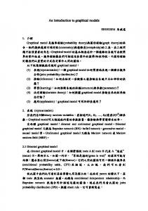
Causal Structure • The flu causes sinus inflamma;on • Allergies also cause sinus inflamma;on • Sinus inflamma;on causes a runny nose • Sinus inflamma;on causes headaches
Causal Structure • The flu causes sinus inflamma;on • Allergies also cause sinus inflamma;on • Sinus inflamma;on causes a runny nose • Sinus inflamma;on causes headaches
Flu
All.
S.I.
R.N.
H
Factored Joint Distribu;on P(F, A, S, R, H) = P(F) P(A) P(S | F, A) P(R | S) P(H | S)
P(F)
Flu
P(S | F, A)
P(R | S)
R.N.
P(A)
All.
S.I.
P(H | S)
H.
A Bigger Example: Star;ng Car • 18 variables • The car doesn’t start. The radio works. • What do we conclude about the “gas in tank”?
Causality and Independence • “A causes B” implies “A and B dependent” • “A and B dependent” does not imply “A causes B”
e.g. smoking, cancer, yellow-‐fingers
15
Querying the Model • Marginal Inference P(F) or P(F|H=t)
Flu
• MAP* Inference
S.I.
argmax f,a P(F=f, A=a|H=t)
• Ac0ve data collec0on In solving one of the two above problems, which variable to query next.
All.
N
H.
* “Maximum Aposteriori,” also someKmes called “MPE Inference” (Most Probable ExplanaKon)
Queries and Reasoning PaRerns • Causal Reasoning or Predic0on
Flu
All.
(downstream)
S.I.
• Eviden0al Reasoning (upstream)
• Inter-‐causal Reasoning
N
(sideways between parents)
“explaining away”
Nothing magical. Underneath everything comes from joint P table.
H.
Reading Independencies from the Graph We used some independencies when building the BN. Once built the BN expresses some independencies itself. How do we read these from the graph?
• N ⊥ F | S (follows from BN def’n)
F
S
S
N
H.
Can we judge independence by the existence of paths with no “blocking” observed variables?
The BN Independence Assump;on again
• Local Markov Assump0on: A variable X is independent of its non-‐descendants given its parents (and only its parents). X ⊥ NonDescendants(X) | Parents(X)
Reading Independencies from the Graph We used some independencies when building the BN. Once built the BN expresses some independencies itself. How do we read these from the graph?
• R ⊥ F | S (follows from BN def’n)
F
A
S
• R ⊥ F | ∅ ? • Answer – Can we imagine a case in which independence does not hold? (reason by converse)
N
H.
Can we judge independence by the existence of paths with no “blocking” observed variables?
A Puzzle • F ⊥ A | S ?
F
P(F)
P(S | F, A)
P(R | S)
N
P(A)
A
S
P(H | S)
H.
A Puzzle • F ⊥ A | S ? P(S|F, A)
F = true, A = true
F
P(F) F = true, A = false
F = false, A = true
F = false, A = false
S = true
0
1
1
0
S = false
1
0
0
1
P(S | F, A)
P(R | S)
N
P(A)
A
S
P(H | S)
H.
A Puzzle • F ⊥ A | S ? P(S|F, A)
F = true, A = true
F = true, A = false
true
0.2
false
0.8 P(F)
F = false, A = true
F = false, A = false
S = true
0
1
1
0
S = false
1
0
0
1
F
P(S | F, A)
P(R | S)
N
true
0.2
false
0.8
P(A)
A
S
P(H | S)
H.
A Puzzle • F ⊥ A | S ? P(S|F, A)
F = true, A = true
F = true, A = false
true
0.2
false
0.8 P(F)
F = false, A = true
F = false, A = false
S = true
0
1
1
0
S = false
1
0
0
1
F
P(S | F, A)
P(R | S)
N
• P(F = true) = 0.2 • P(F = true | S = true) = 0.5 • P(F = true | S = true, A = true) = 0
true
0.2
false
0.8
P(A)
A
S
P(H | S)
H.
A Puzzle • F ⊥ A | S ? • In general, no. – This independence statement does not follow from the Local Markov assump;on.
F
P(F)
P(S | F, A)
P(R | S)
N
P(A)
A
S
P(H | S)
H.
• ¬ (F ⊥ A | S) Discuss Pearl’s “Alarm” network “Explaining away”
Reading Dependencies from the Graph We used some independencies when building the BN. Once built the BN expresses some independencies itself. How do we read these from the graph?
• Direct Connec0on F → S, ¬ F ⊥ S S unob served
• Indirect Causal Effect F → S → H, ¬ F ⊥ H
F
• Indirect Eviden0al Effect H ← S ← F, ¬ H ⊥ F • Common Cause N ← S → H, ¬ N ⊥ H
• Common Effect F → S ← A, S observed ¬ F ⊥ A | S
A
S
N
H.
Reading Independencies from the Graph ¬ F ⊥ S
F ⊥ S
Direct Connec0on X → Y Indirect Causal Effect X → Z → Y Indirect Eviden0al Effect X ← Z ← Y Common Cause X ← Z → Y Common Effect X → Z ← Y
X
Y
X
Z
Y
X
Z
Y
X
Z
Y
X
Z
Y
Z X
“V -‐st
ruc X tu r e” “explaining away”
Z
Z Y
X
Y
Y
X
Y
or an observed descendant!
Z
Ac;ve Trail
“AcKve trail” ~ dependent
Let G be a BN structure and X1 … Xn a trail in G. Let Z be a subset of observed variables. The trail is “ac$ve” given Z if
• whenever we have a v-‐structure Xi-‐1 → Xi → Xi+1, then Xi or one of its descendants are in Z;
• no other node along the trail is in Z. 28
D-‐Separa;on
“Separated” ~ independent
“Directed SeparaKon”
Let X, Y, Z be three sets of nodes in G. We say that X and Y are “d-‐separated” given Z, d-‐sepG(X ; Y | Z), if there is no “ac2ve trail” between any node X ∈ X and Y ∈ Y given Z.
29
D-‐Separa;on Algorithm • Ques;on: Are X and Y d-‐separated given Z? – (How many possible trails?)
1. Traverse the graph boRom up, marking any node that is in Z or with a descendent in Z. 2. Breadth-‐first search from X, only along ac;ve trails; finds reachable set R. – Extra bookkeeping required to keep track of each node being reached via children vs. via parents!
3. X and Y are d-‐separated iff Y ∉ R.
Y
Y
Bayes Ball Algorithm
(due to Ross Shachter)
Another expression of “acKve trails” and d-‐separaKon. X
X
Y
Behavior going from X to Z on path through Y.
Z
X
X (a)
Y
Y
(a)Y
Y
X
Z
Z
X
Y
(b) Z
X
X
(a)(b) X
X
Behavior at end Xpoints.
Z
X
Diagrams from M. Jordan Y
X Z
(a)
X
Y
X
Y
(b)
Y
X
(b)
Y
31
(b)
X1 Y
(b)
Y
(a)
X
Y
(a) (b)
Y
Z(a)
(a)
Y Y
Y
X
Z
(b)
Y X
Z
(b)
X
(a) X
Z
X2
X
X3
X
Y4
X5
D-‐Separa;on and Dependencies Theorem 3.4, (K&F p73): Let G be a BN structure. If X and Y are not d-‐separated given Z in G, then X and Y are dependent given Z in some distribuXon P that factorizes over G.
We use I(G) to denote the set of independencies that correspond to d-‐separaXon: I(G) = { (X ⊥ Y | Z) : d-‐sepG(X ; Y | Z)}. I(G) = the set of independencies guaranteed in all PG
32
What’s Independent? • F ⊥ A | ∅ • A ⊥ F | ∅ • S? • R ⊥ {F, A, H} | S • H ⊥ {F, A, R} | S
P(F)
Flu
P(S | F, A)
P(R | S)
R.N.
P(A)
All.
S.I.
P(H | S)
H.
New Edge: What’s Independent? • F ⊥ A | ∅
P(F)
• A ⊥ F | ∅ • S? • R ⊥ {F, A, H} | S, F • H ⊥ {F, A, R} | S
Flu
P(S | F, A)
P(R | S, F)
R.N.
P(A)
All.
S.I.
P(H | S)
H.
New Edge: What’s Independent? • F ⊥ A | ∅
P(F)
• A ⊥ F | ∅ • • • •
S? R ⊥ {F, A, H} | S, F H ⊥ {F, A, R} | S F ⊥ A | H ?
Flu
P(S | F, A)
P(R | S, F)
R.N.
P(A)
All.
S.I.
P(H | S)
H.
Ques;ons 1. Given a BN, what distribu;ons can be represented? 2. Given a distribu;on, what BNs can represent it? 3. In addi;on to the Local Markov Assump;on, what other independence assump;ons are encoded in a given BN?
Reality vs. Model • World: true distribu;on P – true independencies – true factored form (beyond chain rule)
• Model: Bayesian network – a graph encoding local independence assump;ons
• Any connec;ons?
Representa;on Theorem The condi;onal independencies in our BN are a subset of the independencies in P.
P (X) =
• Given a graph G, can find I(G). • Given a distribu;on P, can find I(P) (in theory anyway) • I-‐Map: I(G) ⊂ I(P) • I-‐Equivalence: I(G1) = I(G2)
n �
i=1
P (Xi | Parents(Xi ))
I-‐Equivalence • Two graphs G1 and G2 are I-‐Equivalent if I(G1) = I(G2) • Define “Skeleton”: undirected version of G. • Theorem 3.7. If G1 and G2 have the same skeleton and the same set of v-‐structures, then they are I-‐equivalent.
39
Minimal and Perfect I-‐Maps • G is a Minimal I-‐Map for I if – G is an I-‐Map for I, and – the removal of any single edge would make it no longer an I-‐Map.
• G is a P-‐Map (Perfect Map) for I if – I(G) = I
• Is there a directed graphical model P-‐Map for every I? – No! 40
Homework #1 • Describe and discuss.
41


![[PDF] Graphical Models - Google Sites](https://m.moam.info/img/260x300/pdf-graphical-models-google-sites_647866f6097c474e708cc5a1.jpg)