Gravitational Collapse of Spherical Interstellar Clouds

PASJ: Publ. Astron. Soc. Japan 5 1 , 637-651 (1999)

Gravitational Collapse of Spherical Interstellar Clouds Shinya

OGINO,

Kohji

TOMISAKA,

and Fumitaka

NAKAMURA

Faculty of Education and Human Sciences, Niigata University, 8050 Ikarashi-2, Niigata, Niigata 950-2181 E-mail (KT): [email protected] (Received 1999 March 24; accepted 1999 July 28) Abstract In this paper, the gravitational collapse of spherical interstellar clouds is discussed based on hydrodynamical simulations. The evolution is divided into two phases: former runaway collapse phase, in which the central density increases greatly on a finite time scale, and later contraction, associated with accretion onto a newborn star. The initial density distribution is expressed using a ratio of the gravitational force to the pressure force a. The equation of state for a polytropic gas is used. The central, high-density part of the solution converges on a self-similar solution, which was first derived for the runaway collapse by Larson and Penston (LP). In the later accretion phase, gas behaves like a particle, and the infall speed is accelerated by the gravity of the central object. The solution at this stage is qualitatively similar to the inside-out similarity solutions first found by Shu. However, it is shown that the gas-inflow (accretion) rate is time-dependent, in contrast to the constant rate of the inside-out similarity solutions. For isothermal models in which the pressure is important, 1 < a < 3.35, the accretion rate reaches its maximum when the central part, which obeys the LP solution, contracts and accretes. On the other hand, in isothermal models in which gravity is dominant, a ^ 3.35, the accretion becomes most active at the epoch when the outer part of the cloud falls onto the center. The effect of the non-isothermal equation of state is discussed. K e y words: Gravitation — Hydrodynamics — Interstellar: clouds — Stars: formation

1.

Introduction

The subject of star formation has attracted much attention. In particular, the relationship between a newborn star and the parent cloud is one of the most important subjects. Since the mid 1960's, the gravitational collapse of clouds has been studied by a number of authors (e.g., Bodenheimer, Sweigart 1968; Larson 1969; Nakano 1979; Boss 1987; Fiedler, Mouschovias 1993; Burkert, Bodenheimer 1993; Ciolek, Mouschovias 1994; Basu, Mouschovias 1994; Tomisaka 1995; Nakamura et al. 1995; Truelove et al. 1998; Bate 1998). For molecular gas with a density lower than 10 10 c m - 3 , radiative cooling is very efficient because the dust opacity is very low. Therefore, the gas is essentially isothermal. Thus, most studies have been performed under the assumption that the gas is isothermal. Many hydrodynamical calculations have shown that the collapse of interstellar clouds proceeds nonhomologously (e.g., Bodenheimer, Sweigart 1968; Larson 1969; Hunter 1977; Foster, Chevalier 1993). Bodenheimer and Sweigart (1968) and Larson (1969) made simulations on the gravitational collapse of spherical clouds which have initially uniform density distributions. They found that even if a cloud is initially uniform, a density gradient develops as the collapse pro-

ceeds. Only the central high-density region essentially collapses because the dynamical time scale, or the local free-fall time, is proportional to ( G p ) - 1 / 2 , where G is the gravitational constant and p is the local gas density. The density is then approximated by a function of the radial distance (r), as p ~ A/(r2 - f a 2 ) , where the coefficient A is constant and the core radius a decreases with time. Moreover, the coefficient A is proportional to the square of the sound speed (cs) and the inverse of the gravitational constant, A oc c 2 /G. These behavior suggests the existence of similarity solutions describing the cloud contraction. One of the similarity solutions for an isothermal spherical cloud was first derived by Larson (1969) and Penston (1969). As the collapse proceeds, the central density increases drastically in a finite time. Consequently, a small dense core, or a protostellar core, is formed at the center. After the core is formed, the envelope gas begins to accrete onto the central core. The accreting gas is accelerated by the gravity of the central core, and its infall speed thus reaches the free-fall one. Then, the radial profiles of the density and velocity follow p oc r - 3 / 2 and v o c r " 1 / 2 , respectively (Boss, Black 1982). The free-falling central region propagates outward as the mass of the central core increases with time. These behavior is also reproduced

© Astronomical Society of Japan • Provided by the NASA Astrophysics Data System

638

S. Ogino, K. Tomisaka, and F. Nakamura

qualitatively by another type of similarity solutions (Shu 1977; Hunter 1977; Whitworth, Summers 1985). These solutions anticipate steady mass-accretion rates onto the central core. Recent multi-dimensional numerical simulations have shown that isothermal clouds with magnetic fields and/or rotation also collapse self-similarly (e.g., Ciolek, Mouschovias 1994; Basu, Mouschovias 1994; Tomisaka 1995, 1996a, 1996b; Nakamura et al. 1995; Matsumoto et al. 1997; Nakamura et al. 1999). This indicates that self-similar collapse is a common feature of isothermal clouds. However, it is only poorly understood how the contraction converges to the similarity solutions. Only a few studies have made quantitative comparisons between the similarity solutions and the numerical results (Foster, Chevalier 1993; Tomisaka 1996a; Matsumoto et al. 1997; Basu 1997; Nakamura et al. 1999). In this paper, we thus examine how the contraction of spherical clouds approaches the similarity solutions. Foster and Chevalier (1993) reexamined the spherical collapse of an isothermal sphere close to hydrostatic equilibrium by using numerical hydrodynamics, and made a comparison between their numerical results and the similarity solutions. They found that the flow in the collapsing sphere approaches the Larson and Penston (LP) solution only near the center before core formation. Most parts of the cloud deviate appreciably from the LP solution because the pressure force significantly retards the contraction in the outer part. As a result, after core formation, the mass-accretion rate declines, contrary to what is expected from the similarity solutions. Their calculations indicate that the collapse depends on the initial condition of the cloud, except in the central small region. In this paper, we extend Foster and Chevalier's (1993) calculations to more general cases. We study how the evolution depends on the initial dynamical state of the cloud because real interstellar clouds are likely to be in various dynamical states. Numerical simulations have also shown that interstellar clouds are prone to fragment into nonequilibrium cores in which gravity is dominant, rather than into cores close to hydrostatic equilibrium (e.g., Tomisaka 1995; Nakamura et al. 1995; Bonnell et al. 1996). We also study the effect of varying the gas equation of state on the cloud collapse because real interstellar gas is not exactly isothermal, and often has appreciable nonthermal internal motions which seem to play an important role in cloud dynamics (e.g., Myers, Fuller 1992). The outline of this paper is as follows. In section 2, we describe our model and numerical methods. The numerical results are given in sections 3 and 4. In section 5, we study the evolution of the mass-accretion rate onto the central core and discuss implications to observations. Finally, in section 6, we summarize our main results.

[Vol. 51,

M o d e l s and N u m e r i c a l M e t h o d s 2.1. Basic Equations and Initial Model To pursue the dynamical collapse of spherical clouds, we constructed a one-dimensional spherically symmetric hydrodynamical scheme. We assume that the system is spherically-symmetric and that the medium consists of ideal gas. The basic equations are then described in the spherical coordinates by dp dt

+

d(pv) dt

1 d(r2pv) dr

+

0

d(r2pv2) dr

(i) GMp

dP_ dr

= 0.

(2)

and

f

47rr'2pdr'

M(r) = M0 + MgAS(r) = M 0 + /

(3)

Jo

where p is the density, v is the radial velocity, P is the pressure, and G is the gravitational constant. The gravitational source comes from two parts: M g a s (the gas mass within radius r) and Mo (the mass of a central point-like object, see subsection 2.2). We assume that the medium is a polytropic gas, :7

-12

I

P

(4)

where 7 is constant and cs denotes the sound speed at the radius at which the density is equal to peq- In this paper, 7 is restricted to 7 < 4/3 because a sphere with 7 > 4/3 is stable to dynamical collapse. The initial models are made in the following manner: (1) The density distribution po(r) is computed by using the hydrostatic equilibrium condition, dP/dr + GMp IT1 = 0. (2) The initial density distribution of the model cloud is assumed to have p(r) = apo(r). This leads to a density by a factor of a higher than that in hydrostatic equilibrium. It is worth noting that a is equal to the ratio of the gravitational force to the pressure force. In the models shown in the present paper, we take po (r = 0) = peq- The initial density at the cloud center is then equal to apeq. We assume that the cloud extends from r = 0 to r o u t . The initial model is then specified by three parameters: a, 7, and r ou t- In our standard model, we set r o u t = 1.82cs/'y/GpecL, which is slightly larger than a critical radius beyond which the isothermal equilibrium sphere is unstable to gravitational collapse (Bonner 1956). The cloud mass and radius are then equal to /

T

\

Mtotal.5.6M.(—j

3 / 2

/

(

p

w

^s)

\-i/2

,


(5)

Gravitational Collapse of Spherical Interstellar Clouds

No. 5]

639

Table 1. Initial conditions of models. a

Model

1.1 4 10 1.1 4 10 1.1 4 10 1.1 4 10 1.1 4 10 1.1 4 10

Al. A2. A3. A4. A5. A6. Bl . B2. B3. B4. B5. B6. CI . C2, C3 C4. C5 C6

and /

T

\1/2 /

routc0.22pc(—)

(

w

^

p = s

)

\-i/2

,

(6)

for the model with a = 1, 7 = 1, and r ou t = 1.82cs/y/Gpeq. In table 1, we summarize the initial conditions of the models calculated in this paper. 2.2. Numerical Methods We solved numerically the one-dimensional hydrodynamical equations (l)-(4) with a TVD Lax-Wendroff code having second-order accuracy in space and time (Davis 1984). We set the fixed boundaries at r = 0 and r ou t- The numerical grid points are non-uniformly distributed so as to enhance the spatial resolution near the center. The grid-spacing increases by 5% for each grid zone with increasing distance from the center. In our standard runs, we used 148 grid points ranging from r = 0 to r o u t • To confirm the effect of varying the spatial resolution, we also calculated several models in table 1 with different numbers of grid points, e.g., 296 and 592 grid points. We found that the numerical results are essentially the same as those with 148 grid points. Many numerical simulations have shown that the collapse of an isothermal sphere accelerates in the central high-density region. The central density increases drastically in a finite time. Thus, the characteristic length and time scales shorten as the collapse proceeds, this phase being referred to as runaway collapse phase. Therefore, it is difficult to resolve the central high-density region sufficiently at the late stages of computation even if we

7 1 1 1 1 1 1 0.8 0.8 0.8 0.8 0.8 0.8 1.2 1.2 1.2 1.2 1.2 1.2

Tout/ y/Gpeq 1.82 1.82 1.82 18.2 18.2 18.2 1.82 1.82 1.82 18.2 18.2 18.2 1.82 1.82 1.82 18.2 18.2 18.2

Psink/Peq 10 6 , 10 6 , 10 6 , 10 6 , 10 6 , 10 6 , 106 106 106 106 106 106 106 106 106 106 106 106

10 13 10 13 10 13 10 13 10 13 10 13

calculate the cloud evolution with very fine grids. However, in real evolution, when the central density reaches ~ 1010 c m - 3 , the effects of dust opacity become important. Cooling radiation can no longer leave the clouds easily. It gets reabsorbed, and the gas begins to heat up. Thus, the assumption of isothermality breaks down, and the equation of state becomes approximately adiabatic. A first hydrostatic core is then formed. When the temperature in the hydrostatic core reaches 2000 K, molecular hydrogen begins to dissociate, resulting in a second collapse within the hydrostatic core. When the dissociation is complete, the collapse is finally stopped with the formation of a second hydrostatic, or protostellar, core (Larson 1969; Bate 1998). After the core formation, the envelope gas begins to accrete onto the central core, and the mass of the central core thus grows in time, this phase being referred to as the accretion phase. To pursue the evolution of the accreting envelope gas, we adopted the sink-cell method when the central density reaches a reference density psink (Boss, Black 1982; Tomisaka 1996a,b). We assign the innermost several cells to sink cells. The excess density (p — psink) and the corresponding momentum are removed from the sink cells in every time step. The removed mass is added to a central point-like object. Mo in equation (3) is equal to the total excess mass removed from the sink cells. Note that Mo is zero before the sink-cell method is applied. We confirmed that the infall near the sink cells is always supersonic during the accretion phase computation. Thus, the structure in the sink cells does not affect the evolution of the envelope. We also calculated several models with



640

i

_ -

1

1

a =4 7=1 r*sink r

out~

7

\ t=nnnn

\ r 1

-4

i

i

i

1

i

\\

ii

i

i

1

0.363

^0 o

1

I

l

l

|

l

I

l

]

V

_ -

1 1 1

-4

y

/

/

\

/

j/

0.326 /

-

1

-2 log(r)

0.329 /

-J

L

l

a.82 1

JH

A\s

I

1 1

(b)

J J

*V

-

i

1

0.631 0.495 ^

= io6/d 1

0.293

i

1

-

J

-

-2

i

(a) J

0.329 0.363 \ \ 0.495 >^\ \ 0.631 \ \ \ \ X

\\ \

V ° 2 l-

i

1

[Vol. 51,

a=4

7=1 1 /W = 1 ° 8 />J ^ = 1-82 1

t=0.293/ l

-6

l

1 l

-4

i

J

i

1

i

i

i

1

i

i

i

1

-2 log(r)

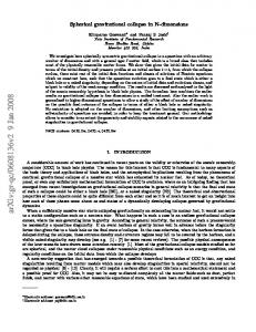
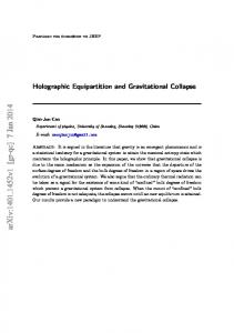
Fig. 1. Radial profiles of (a) density and (b) velocity for the a = 4 isothermal model (model A2). The solid and dashed curves denote the physical quantities before and after core formation, respectively. The number attached to each curve denotes the evolution time from the initial state. In this model, we set p s i n k = 106peq-

different sizes of the sink-cell region and confirmed that the numerical results are essentially the same as those of the models presented in this paper. In the following, we take the central density of a hydrostatic equilibrium cloud (peq) as the unit of density, c s as the unit of velocity, and ( G p e q ) - 1 / 2 as the unit of time. 3.

Collapse of Isothermal Spheres

In this section, we extend Foster and Chevalier's (1993) calculations to more general cases. They studied the collapse of an isothermal sphere close to hydrostatic equilibrium and made a comparison between their numerical results and the similarity solutions. We study the collapse of isothermal spheres in various dynamical states. 3.1. Standard (A 2) Model: a = 4 In this subsection, we investigate the evolution of an isothermal sphere with a = 4 (model A2). Such a nonequilibrium sphere can be formed through the gravitational fragmentation process of a long filamentary cloud without magnetic fields (Tomisaka 1995; Nakamura et al. 1995). In this model, we apply the sink-cell method after the central density reaches 10 6 p e q(= Psink)- When /9eq is taken to be 104 c m - 3 , the density psink is nearly equal to a critical density beyond which isothermality breaks down (psink ~ 10 10 c m - 3 ) . Figure 1 shows the density and velocity distributions of model A2 at seven different stages. The solid and dashed curves denote the radial profiles of the physical quanti-

ties during the runaway collapse and accretion phases, respectively. During the runaway collapse phase, the density profile is nearly uniform in the central part and nearly proportional to r~2 in the envelope. The radial velocity is proportional to r near the center and takes a constant value of ~ 3.3 Cg in the envelope. The central uniform region shrinks in size as the collapse progresses. This evolution seems to be similar to that of the LarsonPenston (LP) solution. After core formation, the density and velocity profiles are proportional to r - 3 / 2 and r - 1 / 2 , respectively, near the center, these values being qualitatively similar to those of the similarity solutions after core formation (Shu 1977; Hunter 1977). To see whether or not the evolution approaches the LP solution, we compared our numerical solutions with the LP solution. The original LP solution derived by Larson (1969) and Penston (1969) is the similarity solution describing the flow during the runaway collapse phase. Hunter (1977, see also Whitworth, Summers 1985) showed that the original LP solution can be extended to the stages after core formation. In the following, this solution extended by Hunter (1977) is referred to as the LP solution. During the runaway collapse phase, the density and velocity distributions of the LP solution are approximated as 1.672 ATTGT2

P= \

8.86c2 I 47rGr2


(7)


641

accuracy of 10% by the stage at which the central density reaches around 30p eq [r ~ — 1.153(Gp eq )~ 1//2 ]. After core formation, the collapse follows the LP solution until (8) about 70% of the cloud mass collapses into the central core [r ~ +0.235(Gp eq )~ 1/2 ]- Thereafter, the evolution 3.28 cs oo deviates gradually from the LP solution. respectively, where r denotes the time measured from To see the effect of varying the threshold density psmk, the epoch of core formation, r = t — to (r < 0 prior to we calculated the evolution of model A2 with a higher core formation). The core formation time t$ is defined as threshold density pSink = 1013peq- The numerical results the time at which the central density reaches an infinite of the models with psink = 1013peq are shown in figure 2 value. We evaluated the core formation time by linear with thin lines. It is found that the evolution is almost extrapolation of pZ (t) because pZ (t) is proportional independent of the value of p i k except at the very late Sn to r when the collapse proceeds self-similarly. stages of the runaway collapse phase (see also subsecDuring the accretion phase, the density and velocity tion 3.2). distributions of the LP solution have qualitatively similar properties to the inside-out similarity solutions found by 3.2. Dependence on a Shu (1977) and are approximated as In this subsection, we discuss the dependence of the evolution on a, comparing all three different sets of cfm 0 1 •0 curves in figures 2 and 3 with each other (models Al, 47rG V 2r 3 r (9) A2, and A3). Our model with a = 1.1 (model Al) is P= \ 8.86c2 essentially the same as the standard model of Foster and oo 2 Chevalier (1993). 47rGr Figures 3a and 3b show the density and velocity proand files during the runaway collapse phase for models Al, 2csm0T A2, and A3. The early evolution depends on a. For the -Cs (10) model with a smaller a, the density profile has a steeper slope in the envelope (p oc r~18, r - 2 , and r~22 for mod-3.28cs oo els A3, A2, and Al, respectively) and the infall speed is respectively, where mo denotes the nondimensional mass- slower in the envelope. However, at the late stages of the accretion rate and is equal to 46.84 for the LP solution runaway collapse phase, both the density and velocity (mo = 0.975 for the inside-out solution by Shu). Note profiles seem to approach a single state near the center. that the density and velocity distributions in the outer This implies that the collapse asymptotically approaches region are the same as those prior to the core formation. the LP solution in the high-density region. Figures 3c and 3d show the density and velocity profiles Figures 2a and 2c show the deviations of pc and the ratio v/r from those of the LP solution [pc,LP and (v/r)i,p], after core formation for models Al, A2, and A3. They respectively, prior to core formation, where pc denotes are plotted at the two stages at which the mass of the the central density. The ratio v/r is defined as a median central core reaches 0.1 Meeq and 0.8 M e q , where M e q of v/r on the 3 grid points nearest to the center. Fig- denotes the mass of the hydrostatic equilibrium sphere The density and velocity ures 2b and 2d show the deviations of pin and i>in from with r o u t = l.S2cs/y/Gpeq. those of the LP solution (pin,LP and t>in,Lp)5 respectively, profiles follow the power laws of p oc r~~3/2 and v oc r - 1 / 2 , after core formation, where the values pin and vm denote respectively, near the center. The regions at which the the density and velocity at the grid point just outside the density and velocity distributions are fitted by power laws sink cells. The solid curves denote the deviations from p oc r~ 3 / 2 and v oc r - 1 / 2 , respectively, widens as the the LP solution for model A2. The deviation of pc from central mass increases in time. It is worth noting that the LP solution is defined as the velocity profiles coincide with the free-fall speed v& = y/2GMcore/r, where Mcore denotes the mass inside the Pc ~ lc,LP Apc = (11) Pc,LP sink cells, and MCOTe = MQ +/ / 4nr2pdr, where rSink Jo The deviations of v/r, pm, and v-m are defined in the is the radius of the sink-cell region. For a comparison, we same manner as the above equation. In the following indicate the free-fall speed v& with dashed-dotted lines we only concentrate at the middle curve in figure 2. (In in figure 3d. The evolution is qualitatively similar to subsection 3.2, we compare all three different set of curves those expected from the similarity solutions after core with each other.) formation. Figure 2 shows that the density and velocity at the To study the approach to the LP solution more quancenter converge on those of the LP solution within an



642 1 1

1

II' li

'%\ ' %

1

1 1 1 1 1 1 1 1 j

•

(a)1 •

| i

p ^

1

4

""•""••••••

1

7=1

10

r

= 10^

j

oUt = 1 - 8 2

i1...._,

1

' 1

7=1 1.82

-0.5

•=ZPsin>=l° pJ

J^33sink

1 1 1 1 1 1 1 11

-2 -4 log(-T)

1

J 6

1 1 11

, i

0.5 h

^0

rAPc -MPC -1

zr~\

J

-2

o

h

-4 I

8

I

-

I

I

6

I

I

I

-

I

4

I

I

I

I

I

I

- 2 log(r)

I

I

0

I

I

L

2

1

1

1

1

1

1

1

1

1

-

1

1

(d) j

K

\ X

_

oo

°2

oo o

0.8 M,

J \o-8^ \ \

=l -\ ^ , = 1.82

r

O.lAf, >*^ ^ V eq

-

0 log(r)

0

^v\%\ \ \ •' Xs-\

'

\ \ \

-J

H J H J

\\: X

i

i

1

i

\

\V4X \i \x a = l.l\

\V3 \\ N

-2

J

1

^ | %

-

-4

H

^§>^_ > ^

0 h

-1

j

i

-2

i

1

i

i

J 1

i

0 log(r)

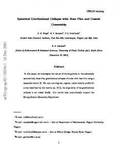
Fig. 3. Density and velocity profiles in the radial direction for isothermal models with a = 1.1 (model A4, dotted curves), 4 (model A5, solid curves), and 10 (model A6, dashed curves). Panels (a) and (c) display the radial density distributions for the runaway collapse phase and the accretion phase, respectively. Panels (b) and (d) are for infall velocities in the runaway collapse phase and the accretion phase, respectively. In panels (c) and (d), two stages are plotted at which the mass of the central core (MCOre) reaches 0.1 M e q and 0.8 M e q . In panel (d), free-fall speeds vg = (2GM C O re/^) - 1 / ' 2 are shown by dashed-dotted lines.

the runaway collapse similarity solutions except the LP solution are very unstable to spherical perturbations (see also Ori, Piran 1988; Silk, Suto 1988). Therefore, it is expected that if the spherical collapse always proceeds self-similarly, the flow must approach the LP solution. When a is closer to 4, the region which obeys the LP solution is wider. For the models with a = 4, 1.1, and 10 (models A2, Al, and A3), the central regions with a mass of 0.7M tot ai, 4 x 10~ 3 M to tai, and 2 x 10" 5 M to tai can be approximated by the LP solution within an accuracy of 20% at the epoch of core formation, respectively.

Here, Mtotai denotes the total mass of the cloud. This is related to the fact that the ratio of the gravitational force to the pressure force is nearly equal to 4 for the LP solution. Therefore, the evolution of model A2 is better approximated by the LP solution even in later stages than those of models Al and A3. In figure 2, there is small deviation between thick (Psink = 106peq) and thin (1013/9eq) lines for each model with the same a during the runaway collapse phase. The deviation is mainly due to the difference in the core formation time to we used for thick and thin lines. As men-



644

1

1

1

1

1

[Vol. 51,

1

1

1

1

1

1 1

l

1 1

(b)

sink

2.958 2.958^ \ 2.458^^^^

"eq

so o

0h 2.362/

2.359 /

/

/

/

\

a==1

/

/

.1

J

7=1

/

"sink

/

1

out

= 1.82 J

i

1

i

2.317

-4

-2 log(r)

0

1

-6

i

i

1

-4

i

i

i

1

i

i

i

i

l

-2 log(r)

Fig. 4. Same as figure 1, but for the model with a = 1.1 and 7 = 0.8 (model Bl). Radial profiles of (a) the density and (b) velocity.

tioned in the previous subsection, we evaluated the core— 1/2

formation time by linear extrapolation of pc (t). If the collapse converges to the LP solution, then the evaluated core-formation time will coincide with the core-formation time expected from the LP solution. In reality, the degree of convergence depends on the adopted value of pSink, i.e., the stages at which we evaluated the core-formation time to. Since the collapses near the center do not converge completely to the LP solution during the runaway collapse phase for all the models calculated in this paper, the evaluated values of to are slightly different from those for the models with different pSink- This difference causes a deviation between the thick and thin curves for each model having the same a. The deviation is largest for model Al because the convergence to the LP solution is slowest for a given r. This slow convergence comes from the dominant pressure effects of model Al. 4.

Collapse of Polytropic Spheres

In the previous section, we considered the collapse of spherical clouds under the assumption that the interstellar gas is isothermal. However, observations have shown that real interstellar gas is not exactly isothermal. Observed cloud cores also have appreciable nonthermal internal motions which are thought to be due to interstellar turbulence. Myers and Fuller (1992, 1993; also Caselli, Myers 1995; Maloney 1988) modeled the turbulent pressure as that of a polytropic gas with 7 < 1. The pressure of such a polytropic gas seems to reproduce well that of observed nonthermal motions [see also Lizano and Shu (1989) and McLaughlin and Pudritz (1996, 1997) for the

other type of the equation of state]. Recently, VazquezSemadeni, Canto, and Lizano (1998) also made a numerical simulation of a turbulent isothermal cloud undergoing gravitational collapse. They found that the turbulent gas seems to behave as a polytropic gas with 7 > 1 when the turbulent motions do not dissipate appreciably during gravitational collapse. Thus, in this section, to clarify the effect of the equation of state, we investigate the evolution of polytropic spheres. When 7 > 4/3, the cloud is stable to gravitational collapse. We thus restrict 7 to 7 < 4/3 in this paper. 11. Effect of 7 Figures 4 and 5 show the evolutions of the density and velocity profiles for models Bl and CI, respectively. For these models, we apply the sink-cell method after the central density reaches psm^ = 106peq- Prior to core formation, for the model with a large 7, the uniform central region is wider, and the density distribution in the envelope is steeper at the stages at which the central density reaches the same value (p oc r ~ 2 6 and r - 1 8 for models CI and Bl, respectively). This power-law distribution of the density is qualitatively similar to that of the similarity solutions for a polytropic sphere. For the similarity solutions of polytropic spheres, the density profile is proportional to r - 2 ^ 2 - 7 ^ in the envelope (p oc r - 2 5 and r - 5 / 3 for models CI and Bl, respectively. See, e.g., Larson 1969). On the other hand, once the core forms at the center, the density and velocity profiles at the inner region follow the power laws of p oc r - 3 / 2 and v oc r - 1 / 2 , respectively. Such behavior is similar to that of the isothermal



No. 5]

-i

1

r-

I

1.50 &08\

1.506

'

'

1

'

1

1

1

1

1

1

1

645

i

1

T " "[ •

(a) j

\^ 1.562\

V ^ A

1

1

1

(b)

a = l.l 7 = 1.2

-

r _ = 1.82 ^

-

H

1.766 1.562^^ 1.508\

^ °2

L_

00

1.412

o

-

_2 i - 6

-2 — h

t=0.000-

i

i

i

I i - 4

i

i

I • - 2

i

i

I' i 0

i_

-4

log(r)

|

0 h 1.506

L_

1

1

-6

a = l.l

/

I

7=12 1.499 /

/

1A12' , , 1 ,

.

„A

/°»i n Jc= 106 /°J

.

l

1

I

1

1

1

I

1

-2 log(r)

Fig. 5. Same as figure 1, but for the model with a = 1.1 and 7 = 1.2 (model CI).

model. The region at which the p oc r~ 3 / 2 and v oc r - 1 / 2 profiles are applicable becomes wide outwardly as the collapse proceeds. This behavior is also similar to that of the similarity solution of a polytropic sphere after core formation. It is worth noting that for the model with 7 ~ 0.6, the power index of the density profile does not change during the contraction. Therefore, for the model with 7 ~ 0.6, it is very difficult to distinguish the evolution phases of cloud contraction (i.e., prior to and after core formation) from the density profile. 4.2. Approach to the LP-Type Solution As shown in the previous subsection, polytropic spheres seem to collapse self-similarly. Several authors have also obtained similarity solutions for a polytropic sphere (Larson 1969; Cheng 1978; Goldreich, Weber 1980; Yahil 1983; Suto, Silk 1988; Blottiau et al. 1988; McLaughlin, Pudritz 1997). In the following, we investigate how the evolution asymptotically approaches the similarity solutions for a polytropic sphere. The similarity solutions for a polytropic sphere show that in the runaway collapse phase, the central density evolves in proportion to r - 2 , and the velocity near the center evolves as v/r = 2/(3r). Unfortunately, we do not know the proportional coefficients of the central density for the similarity solutions with 7 ^ 1 [cf. equation (7) for the isothermal models]. To compare the numerical results with the similarity solutions, we thus measured the nondimensional central density, 47rGpcr2, (figures 6a and 6c for the models with 7 = 0.8 and 1.2, respectively) and the deviation of v/r from the similarity solutions (figures 6b and 6d for the models with 7 = 0.8 and 1.2, respectively), where the nondimensional central density

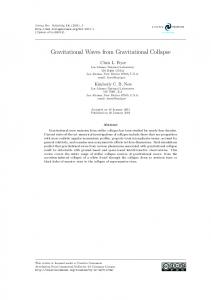
stays constant if the evolution converges to the similarity solution. Figure 6 indicates that for the models with the same 7, the nondimensional central densities seem to asymptotically approach a single constant value, irrespective of a. For the models with 7 = 0.8 and 1.2, the asymptotic values are expected to be nearly equal to 47rGpcr2 = 0.765 ± 0.07 and 6.93 ± 0.35, respectively. The deviation of the velocity from the similarity solution is also very small for both models. We have also calculated the evolutions of the models with different 7 in the range o f 0 . 8 < 7 < 1 . 2 , finding that the asymptotic value of the nondimensional central density smoothly approaches the LP value as 7 —> 1. In other words, the collapse of a polytropic sphere asymptotically approaches the LP-type solution. 5.

Mass-Accretion Rates

In this section, we discuss the evolution of the massaccretion rate onto the central core. For all the models in this section, we apply the sink-cell method when the central density reaches psink = 106/9eq5.1. Isothermal Clouds Figure 7 shows the evolutions of the mass-accretion rates for models Al, A2, and A3. The thick solid curves denote the models with r o u t = 1.82cs/^s/Gp^. For all models, the difference of M is not very large at the early stages (r < 10" 3 , M - 50±30c 3 /G for 1 < a < 10). This is because the central region has approached the LP solution just before core formation. However, later evolutions are different from each other. For model A2, the mass-



646

r

it

i

• |

i

i

i

|

i

i

i

|

i

-i—I—i—i

i

.

1

[Vol. 51,

i

1

r-

1 I 1

*

\

1.5 -h

(b)

(a>

\«=i.i

r-o.a

\

j

7=0.8 Vl.82

roul=1.82 1

1 1 1 1.. 1—1

loW^^I^B-

L

j

~ ^ *

0.5 h

r, i

. . .

1 . . .

1 . . .

-2

1 .

-4

-6

10

-I—1—1 1

lOg(-T)

|

-

...1 — L

1 1 1 1 1

j

1

]

>

1

1

.

1 1

i— r

T — | — T

(d) 7=1.2 J 'out-1-82 1

-

•

•

!

>

-6

if

-j

\4 MI10

f -1

•]

^ - T < ^ ^

'0 h

A/>c=io /w 1

1

-

-0.5 H

-2 -4 log(-r)

1

0.5 h

. ..

I . I

1

a = l.l

_ -

8

10

1

1

r oul =l-82

V/ 1

-1

1

\

7=1.2

i */y

1 1

1

1

(c)

1 - I"l

|

/*'

6 h

2 h

1

"""*-.^ «...

-

^

1

.. a = 1.1

8 h

^ §fc

1

1

/ f 1 1,1 , ,

J

] 1 , , , 1 -2 -4 lOg(-T)

...1.1 -6

Fig. 6. (a) Nondimensional central density 47rGpcr2 and (b) Av/r as a function of r for the models with 7 = 0.8 (models B l , B2, and B3). (c) 47cGpcT2 and (d) Av/r as a function of r for the models with 7 = 1.2 (models CI, C2, and C3). Both are for the runaway collapse phase. Solid, dashed, and dotted curves denote the models with a = 4, 10, and 1.1, respectively. The filled circles, triangles, and squares denote the stages at which the central density reaches 10 3 , 10 6 , and 10 9 p e q , respectively.

accretion rate stays nearly constant at M ~ 50cj?/£? until the central region with a mass of about 0.7 M to tai accretes onto the central core. This indicates that, for this model, the central region with a mass of about 0.7 M to tai converges to the LP solution by the epoch of core formation. After the central region with a mass of 0.7 Mtotai collapses into the central core, the mass-accretion rate declines below the LP value because almost all the cloud mass has already collapsed into the central core. On the other hand, the mass-accretion rates for models Al and A3 begin to deviate appreciably from the LP solution at earlier stages than for model A2. [From the numerical

results of the models with psink = 1013peq5 we found that at the very early stages (r < 10 - 4 ), the accretion rates of models Al and A3 nearly coincide with the LP value, beginning to deviate from the LP value as the collapse proceeds. This behavior is not remarkable for the models with psink = 106peq-] For the models with large a, M becomes larger than the LP value, while for the models with small a, it declines below the LP value. It is therefore concluded that the evolution of the mass-accretion rate depends strongly on the initial condition. To clarify the evolution of the mass-accretion rate, we measured the maximum of the mass-accretion rate as a



No. 5]

647

300

200

I 100

0.2

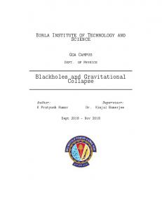
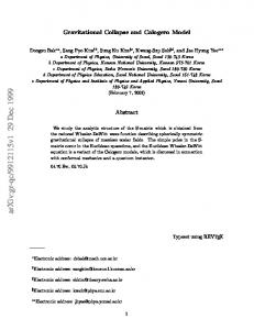
log(r) Fig. 7. Mass-accretion rates as a function of r for the isothermal models with a — 1.1, 4, and 10 (models A l , A2, A3, A4, A5, and A6). The unit of the mass-accretion rate is taken to be Cg/G, which is equal to 1.6 x 1 0 - 6 M® y r _ 1 for T = 10 K. The unit of time is taken to be l / ^ / G p e q , which is equal to 6.3 x 10 5 yr for peq = 10 4 c m - 3 . Thick and thin solid curves denote the models with ^out = l.82cs/\/Gpeq (models A l , A2, and A3) and 18.2c s /\ZGp e q (models A4, A5, and A6), respectively. The filled circles, triangles, and squares denote the stages at which the mass of the central core reaches 0.1 M t o t a i , 0.5 M t o t a i , and 0.8 M to tai> respectively. For a comparison, the mass-accretion rates of the pressure-free model and the LP solution are plotted by dotted and dashed-dotted lines, respectively.

0.4

0.6 0.8 log (a)

1.2

Fig. 8. Maximum of mass-accretion rate as a function of a for the models with various 7. The unit of the mass-accretion rate is taken to be cf/G, which is equal to 1.6 x 1 0 - 6 M® y r - 1 for Cs = 0.19 km s _ 1 (T = 10 K). The unit of time is taken to be 1/y/Gpeq, which is equal to 6.3 X 10 5 yr for peq = 10 4 c m - 3 . The number attached with each line denotes the value of 7. For each line, we calculated many models with different a, i.e., a = 1.1,1.5, 2, 2 . 5 , . . . , 10.

those models are shown by thin solid curves in figure 7. For the models with a large radius, the mass-accretion rates converge well to those of the pressure-free model at the late stages of the computation (see figure 7). This is particularly true for models A5 and A6, in which the gravity is dominant in the envelope. function of a, which is shown in figure 8. In this subsecThe evolution of the mass-accretion rate for the tion we only concentrate at the curve with 7 = 1. (In pressure-free cloud is expressed by equation (A7). When subsection 5.2, we compare all four different sets of curves 7 = 1, the density distribution in the envelope is nearly with each other.) For the isothermal models in which proportional to r~2 [p ~ ac%/(2irGr2)] and, therethe pressure is important, l < a < 3 . 3 5 , the maximum fore, the mass within radius r is nearly proportional accretion rate depends only weakly on a (Mmax oc a 1 / 5 ) to r (M rsj 2ac2r/G). Thus, the mass-accretion rate exand is close to the LP value ( M L P — 47Cg/G). On the pected from the pressure-free model is nearly constant, other hand, for the isothermal models in which the grav- M ~ 7ra3/2Cg /G, while the power-law envelope mass conity is dominant, a > 3.35, the maximum accretion rate tinues to accrete onto the central body, r > 10. exceeds the LP value and increases in proportion to a 3 / 2 . This dependence of M(oc a 3 / 2 ) can be reproduced by 5.2. Dependence on 7 a pressure-free collapse model for all the models with Figure 9 shows the mass-accretion rates as a function a ti 3.35. In the Appendix, we derived the mass-accretion of r for the models with 7 = 0.8, 1, and 1.2. The rate for the pressure-free sphere as a function of time. For mass-accretion rate strongly depends on 7. For the moda comparison, in figure 7, the time evolution of the mass- els with 7 = 1.2 (models CI, C2, and C3), the massaccretion rate for the pressure-free sphere is shown with accretion rates reach their maxima just after core fordotted curves. mation. The maximum of M depends only weakly on a To see the effect of cloud size, we calculated the evo- (see figure 8). These maxima of M are expected to be lution of models A4, A5, and A6, which have 10 times nearly equal to the accretion rate of the LP-type solution larger radii (r ou t = 18.2cs/-\/Gpe(i). The evolutions of for 7 = 1.2 because the central part seems to converge


648


[Vol. 51,

auu

«-10

/(b)

-]

7=12\ 400

200

/ 100

n

-4

2

;

1 i

J

,/^^\TV

J

0.8

-

-

\ i

1.2

.

1 8

L.I 1 i . 1

-

.u.=

.1. 1

300

r

k

__J / ^ 0.8

\\

1 1_... J

-2

J

1

^^.^-^

V

1

-T-»-J

0

H l

log(r) Fig. 9. Dependence of the mass-accretion rates on 7 for (a) the a = 1.1 and (b) a = 10 models. The unit of the massaccretion rate is taken to be cf /G, which is equal to 1.6 x 1 0 - 6 M® y r _ 1 for Cg = 0.19 km s - 1 (T = 10 K). The thick and thin solid curves denote the models with r o u t = e q and 18.2c s /A/Gpeq, respectively. For a comparison, the mass-accretion rate of the pressure-free model is shown by dotted curves.

well to the LP-type solution just before the core formation (see figure 6). The maximum of M is much larger compared to the other models with smaller 7 because the sound speed near the center increases with increasing central density when 7 > 1. After the mass-accretion rate reaches its maximum, it quickly declines. On the other hand, for the models with 7 — 0.8 (models Bl, B2, and B3), the evolution of M is very different from that of the 7 = 1.2 models. The mass-accretion rate increases at the later stages of the computation, in particular, when the cloud has an extended envelope and a is large. Such evolution is explained as follows. At the late stages, the evolution of the mass-accretion rates is reproduced well by the pressure-free model, particularly for models with a large a, in which gravity is dominant. For the models with a small a, the mass-accretion rates of the pressure-free model do not fit those of the numerical solutions well during the computation because the pressure force plays a significant role in the contraction. For a comparison, we show M of the pressure-free model with the dotted lines in figure 9. In the pressure-free model, the evolution of M depends on the initial density distribution (see the Appendix). For polytropic clouds, the density distribution in the envelope is nearly proportional to p oc r ~ 2 / ( 2 - 7 ) . Then, when the envelope gas at the initial radius #0 accretes onto the center, the massaccretion rate is expected to be nearly proportional to M (xRt2(l- 7 )/(2-7) . Hence, for 7 > 1 (7 < 1), the massaccretion rate decreases (increases) with time as long as the envelope gas accretes onto the center. See also fig-

ures 8 and 9 and equation (A8) in the Appendix. 5.3. Implications to Observations As shown in the previous subsections, the massaccretion rate is time-dependent, and its evolutional path depends both on a and 7. Thus, comparing our numerical results with observations, we can specify the parameters a and 7 and determine the evolutional path of observed cloud cores from the evolution of M. Observationally, the amount of the envelope-gas mass (M e n v = -Mtotai — Afcore) is likely to be a good indicator of the evolutional stage of an observed isolated cloud core because M e n v monotonicly decreases with time owing to accretion onto a central protostar. [If the cloud cores interact with each other, then the accretion of the envelope gas may be influenced by the interaction and tidal torque. See, e.g., Bonnell et al. (1997) and Klessen et al. (1998).] In the following, we thus obtain the mass-accretion rate as a function of M e n v • Figure 10 shows the mass-accretion rates as a function of the envelope mass normalized by the total cloud mass (M env /Mtotai) for several models calculated in the previous sections. The mass-accretion rates of all the models in figure 10 are calculated until 80% of the total mass accretes onto the central core. The evolutional path of M depends mainly on a except at the very early stages. Although the very early evolution of M is remarkably different for the models having different 7, it may be difficult to observe the early evolution of M because of a short evolution-time scale (At < 104 yr for p e q = 105 c m - 3 ) . During the accretion phase, there is no


No. 5]


-|—i—i—|—i—i—i—|—i—i—i—|—i—i—i—|—i—i—i—|—r

-7=0.8 _.-*-

-0.6

-0.4

•"31

-

\og(AM/MloU1) Fig. 10. Mass-accretion rate as a function of envelope mass normalized by total cloud mass. The solid, dashed, and dotted curves denote the massaccretion rates for the models with 7 = 1, 0.8, and 1.2, respectively. The filled circles denote the stages at which the evolution time is equal to t — O.l(aGpeq)-1/2, O ^ a G p e q ) - 1 7 2 , 0 . 3 ( a G p e q ) - 1 / 2 , . . . , where apeq denotes the initial central density.

appreciable change in the mass-accretion rates of any of the models, except at the very early stages. Observed young stellar objects (YSOs) are often classified into several empirical evolutional stages from starless dense core to main sequence star (e.g., Andre et al. 1993). The youngest observed YSOs are called Class 0 sources, which are interpreted to be in a phase at which the envelope gas still has more mass than the central hydrostatic protostellar core. More evolved YSOs are called Class I sources. Recently, Bontemps et al. (1996) and Henriksen et al. (1997) suggested that if the CO outflow rate is proportional to the mass-accretion rate onto the central star, the mass-accretion rates of Class 0 sources are a factor of 10 larger on average than those of Class I sources. This implies that the mass-accretion rate is time-dependent, contrary to the standard theory of star formation by Shu and coworkers (e.g., Shu et al. 1987). They also suggested that mass-accretion history may vary from region to region; in the p Ophiuchi region, the accretion rates of Class 0 sources decline with time, while in Taurus, they stay nearly constant during Class 0 and Class I phases. Constructing a simplified pressure-free spherical collapse model, Henriksen et al. (1997) proposed that in the p Ophiuchi region, the observed dispersion of M for Class 0 sources is due to the time evolution of M. In our hydrodynamical model, however, pressure force plays an important role in dynamical evolution and significantly retards the rapid change of M

649

when the central region accretes onto the central core. In other words, even for the models with large a (~ 10), the pressure-free model is not applicable at the early stages of the accretion phase. By a comparison with figure 7 of Henriksen et al. (1997), we thus suggest that the dispersion of the accretion rate for Class 0 sources comes mainly from the different initial dynamical state (i.e., various a) if the variation of the gas temperature is not important. Therefore, for Class 0 sources in the p Ophiuchi region observed by Bontemps et al. (1996), the parent cloud cores may have been in various dynamical states (various a ) , while, in Taurus, they may be close to hydrostatic equilibrium (a~l). In the above scenario, it seems difficult to explain the difference of M between Class 0 sources and Class I sources except for the a ~ 1 models. [In our models with a — 4 and 10, M does not change appreciably as M e n v decreases (see figure 10).] This difference may come from their different accretion mechanisms. In Class 0 phase, gas infall is more dynamical than that in Class I phase. Thus, outflow rate driven by dynamical infall is expected to be high because of high accretion rate (M ~ 10-5M@) yr" 1 ; see Tomisaka 1998). On the other hand, in Class I phase, outflow is likely to be driven by viscous accretion of a centrifugally supported disk near the central star, the rate of which is expected to be a factor of 10 smaller than that of the dynamical model (M ~ 10~ 6 M® y r - 1 ) . This implies that the outflow rate of Class I sources is a factor of 10 smaller than that of Class 0 sources if the outflow rate is nearly proportional to the accretion rate and its proportional coefficient does not change significantly in both the Class 0 and Class I phases. 6.

Summary

We studied the gravitational collapse of isothermal and polytropic spherical clouds in various dynamical states. For both isothermal and polytropic models, the flow near the center asymptotically approaches the LP-type solution reaching core formation, irrespective of the initial conditions. The density profile in the envelope follows the power-law distribution p oc r~2^2~y\ When the ratio of the gravitational force to the pressure force is closer to that of the LP-type solution at the initial state, the flow near the center converges to the LP solution at the earlier stages of the contraction. At the epoch of core formation, the central regions with a mass of 0.7 Mtotai5 4 x 10~ 3 M to tai 7 and 2 x 10~ 5 M to tai have converged to the LP solution within an accuracy of 20% for the isothermal models with a = 4, 1.1, and 10 (models A2, Al, and A3), respectively. The evolution of model A2 quickly converges to the LP solution. If spherical cores are formed through the gravitational fragmentation of a long fila-


650


mentary cloud, then they are likely to have a ~ 4 (e.g., Tomisaka 1995; Nakamura et al. 1995). Thus, for such a core, the LP solution is applicable to the core as a whole. After core formation, until the region converging to the LP solution by the epoch of core formation accretes onto the central core, the flow can be approximated by that of the LP solution. Thereafter, the flow appreciably deviates from the LP solution. The subsequent flow is determined mainly by the initial conditions. Thus, after the region converging to the LP solution accretes onto the central core, the mass-accretion rate becomes time-dependent, in contrast to the constant rate of the similarity solutions. In the isothermal models in which the pressure is important ( l < a < 3 . 3 5 ) , the mass-accretion rate reaches its maximum when the central region which obeys the LP solution accretes onto the central core. On the other hand, in the isothermal models in which the gravity is dominant (a > 3.35), the accretion is very high and reaches its maximum at the stages at which the outer part of the cloud accretes onto the center. If the isothermal cloud has a very extended envelope, then M tends to approach a constant rate which depends on a. The evolution of the mass-accretion rate depends strongly on 7. When 7 > 1, M reaches its maximum at the early stages and quickly declines thereafter. On the other hand, when 7 < 1 and the cloud has an extended envelope, M increases with time and thus reaches its maximum at the nearly final stage of the computation. The later evolution of M can be approximated by the pressure-free model except for the models with a ~ 1. By a comparison with figure 7 of Henriksen et al. (1997), we suggest that the dispersion of the massaccretion rate for Class 0 sources comes mainly from the different initial dynamical state (i.e., various a) if the variation of the gas temperature is not important. We are grateful to T. Hanawa for useful discussions on the similarity solutions for a polytropic sphere. We also thank an anonymous referee for valuable comments that improved the paper. Numerical computations were carried out on VX/4R at the Astronomical Data Analysis Center of the National Astronomical Observatory. This work was financially supported by Grants-in-Aid for Scientific Research of the Ministry of Education, Science, Sports and Culture (10147105, 10147205, 11134203, 11640231). Appendix. Mass-Accretion Rate of a PressureFree Sphere Here in this appendix, a formula to estimate the massaccretion rate is given assuming that a cloud contracts in a free-fall manner (pressure-free cloud, see also Henriksen

[Vol. 51,

et al. 1997). The equation of motion for a mass-shell is written in terms of the distance from the center R as GM(Rp) R* '

dR dt

(Al)

where RQ represents the distance at the epoch of t — 0 and M{R) indicates the mass included within the distance R as

f

M(R)

4nr pdr.

(A2)

Jo the mass-shell is initially static, the total Assuming that (kinetic 4- potential) energy of the system must be negative. In this case, the motion for a mass-shell R(t) whose initial position was R = RQ at t — 0 can be expressed using a parameter 0 as 1/2

Ro [2GM(Ro)

Ro(6 + sm6)

(A3)

and R =

Ro(l + cosQ)

(A4)

0 = 0 corresponds to the initial state (R = Ro and t — 0), while 6 = ir represents the epoch at which the shell reaches the center R = 0. Therefore, the necessary time for a mass-shell at Ro to reach the center (free-fall time) is expressed as T(Ro) =

Ro 2GM{Ro)

1/2

nRo

(A5)

Consider two shells whose initial radii are equal to Ro and Ro + ARQ. The time difference for these two shells to reach the center AT(Ro) can be expressed using equation (A5) as AT(Eo) =

7T.Ro

1/2

2 3 / 2 [GM(#o)] 1 / 2 3 RQ dM(Ro) AiJo. 2 ~ 2M(Ro) dRo J

(A6)

The mass in the shell between #0 and Ro + A,Ro, A M = M(Ro + ARo) - M(Ro) = (dM/dRo)ARo, accretes on the central object in AT(Ro). Thus, the mass-accretion rate for a pressure-free cloud is expressed as AM/AT. This leads to the expression as

£

2 3/2

X

Gl/2M(J?())3/2

Ro3/2 Ro dM(Ro) M(RQ) dRp 3 RQ dMjRy) 2 ~ 2M(Ro) dRo

'


(A7)

No. 5]


Coupled with equation (A3), this gives the time variation of t h e accretion rate. Typical time variations are plotted in figure 7. Consider two clouds with the same density distribution dlogp/dr b u t different a, as t h e models shown in figure 7. Since these two clouds have the same d\ogM(Ro)/d\ogRo, the mass-accretion rate depends only on M(RQ)/RQ and is expressed as

dM (Ro)oc IT

M(R0) JRO

3/2

oc a

3/2

(A8)

This indicates t h a t the accretion r a t e is proportional t o a 3 / 2 , while t h e time scale is proportional to a - 1 / 2 . This seems to correspond to t h e fact t h a t t h e m a x i m u m accretion rate is well expressed in proportion to a 3 / 2 for models a > 3.35 (7 = 1). W h e n t h e initial density distribution is t h e singular isothermal sphere (Chandrasekhar 1939) as p oc r ~ 2 , t h e mass included inside Ro is proportional to radius M(Ro) oc Ro. Since T(RQ) oc R30/2/M(Ro)1/2, t h e freefall time is also proportional t o Ro. In this case, equation (A7) gives a constant accretion rate in time. References Andre P., Ward-Thompson D., Barsony M. 1993, ApJ 406, 122 Basu S. 1997, ApJ 485, 240 Basu S., Mouschovias T.Ch. 1994, ApJ 432, 720 Bate M.R. 1998, ApJ 508, L95 Blottiau P., Bouquet S., Chieze J.P. 1988, A&A 207, 24 Bodenheimer P., Sweigart A. 1968, ApJ 152, 515 Bonnell I.A., Bate M.R., Clarke C.J., Pringle, J.E. 1997, MNRAS 285, 201 Bonnell LA., Bate M.R., Price N.M. 1996, MNRAS 279, 121 Bonner W.B. 1956, MNRAS 116, 351 Bontemps S., Andre P., Terebey S., Cabrit S. 1996, A&A 311, 858 Boss A.R 1987, ApJ 319, 149 Boss A.R, Black D.C. 1982, ApJ 258, 270

651

Burkert A., Bodenheimer P. 1993, MNRAS 264, 798 Caselli P., Myers P.C. 1995, ApJ 446, 665 Chandrasekhar S. 1939, Introduction to the Study of Stellar Structure (University of Chicago Press, Chicago) sect22 Cheng A.F. 1978, ApJ 221, 320 Ciolek G.E., Mouschovias T.Ch. 1994, ApJ 425, 142 Davis S.F. 1984, NASA Contractor Report 172373, ICASE REPORT No. 8420 Fiedler R.A., Mouschovias T.Ch. 1993, ApJ 415, 680 Foster P.N., Chevalier R A . 1993, ApJ 416, 303 Goldreich P., Weber S.V. 1980, ApJ 238, 991 Hanawa T., Nakayama K. 1997, ApJ 484, 238 Henriksen R., Andre P., Bontemps S. 1997, A&A 323, 549 Hunter C. 1977, ApJ 218, 834 Klessen R.S., Burkert A., Bate M.S. 1998, ApJ 501, L205 Larson R.B. 1969, MNRAS 145, 271 Lizano S., Shu F.H. 1989, ApJ 342, 834 Maloney P. 1988, ApJ 334, 761 Matsumoto T., Hanawa T., Nakamura F. 1997, ApJ 478, 569 McLaughlin D.E., Pudritz R.E. 1996, ApJ 469, 194 McLaughlin D.E., Pudritz R.E. 1997, ApJ 476, 750 Myers P . C , Fuller G A . 1992, ApJ 396, 631 Myers P . C , Fuller G A . 1993, ApJ 402, 635 Nakamura F., Hanawa T., Nakano T. 1995, ApJ 444, 770 Nakamura F., Matsumoto T., Hanawa T., Tomisaka K. 1999, ApJ 510, 274 Nakano T. 1979, PAS J 31, 697 Ori A., Piran T. 1988, MNRAS 234, 821 Penston M.V. 1969, MNRAS 144, 425 Shu F.H. 1977, ApJ 214, 488 Shu F.H., Adams F . C , Lizano S. 1987, ARA&A 25, 23 Silk J., Suto Y. 1988, ApJ 335, 295 Suto Y., Silk J. 1988, ApJ 326, 527 Tomisaka K. 1995, ApJ 438, 226 Tomisaka K. 1996a, PAS J 48, L97 Tomisaka K. 1996b, PASJ, 48, 701 Tomisaka K. 1998, ApJ 502, L163 Truelove J.K., Klein R.I., McKee C.F., Holliman J.H. II, Howell L.H., Greenough J.A., Woods D.T. 1998, ApJ 495, 821 Vazquez-Semadeni E., Canto J., Lizano S. 1998, ApJ 492, 596 Whitworth A., Summers D. 1985, MNRAS 214, 1 Yahil A. 1983, ApJ 265, 1047
