Green and energy efficiency in access networks and cloud ...

Green and energy efficiency in access networks and cloud infrastructures Ahmed Amokrane

To cite this version: Ahmed Amokrane. Green and energy efficiency in access networks and cloud infrastructures. Mobile Computing. Universit´e Pierre et Marie Curie - Paris VI, 2014. English. .

HAL Id: tel-01150569 https://tel.archives-ouvertes.fr/tel-01150569 Submitted on 11 May 2015

HAL is a multi-disciplinary open access archive for the deposit and dissemination of scientific research documents, whether they are published or not. The documents may come from teaching and research institutions in France or abroad, or from public or private research centers.

L’archive ouverte pluridisciplinaire HAL, est destin´ee au d´epˆot et `a la diffusion de documents scientifiques de niveau recherche, publi´es ou non, ´emanant des ´etablissements d’enseignement et de recherche fran¸cais ou ´etrangers, des laboratoires publics ou priv´es.

` THESE DE DOCTORAT DE ´ l’UNIVERSITE PIERRE ET MARIE CURIE Sp´ecialit´e Informatique Ecole doctorale Informatique, T´el´ecommunications et Electronique (Paris)

Pr´esent´ee par

Ahmed AMOKRANE Pour obtenir le grade de ´ PIERRE ET MARIE CURIE DOCTEUR de l’UNIVERSITE

Sujet de la th`ese :

Green et Efficacit´ e en Energie dans les R´ eseaux d’Acc` es et les Infrastructures Cloud

Soutenance le 8 D´ecembre 2014 Devant le jury compos´e de : Pr. Dr. Pr. Dr. Dr. Pr. Pr. Dr.

Olivier Festor Nathalie Mitton Raouf Boutaba Jin Xiao Marcelo Dias de Amorim Jean-Louis Rougier Guy Pujolle Rami Langar

Rapporteur, INRIA Nancy, France Rapporteur, INRIA Lille-Nord Europe, Lille, France Examinateur, University of Waterloo, Ontario, Canada Examinateur, IBM Research, T.J. Watson, New York, USA Examinateur, UPMC (Paris 6), France Examinateur, Telecom ParisTech, Paris, France Directeur de th`ese, UPMC (Paris 6), France Co-directeur de th`ese, UPMC (Paris 6), France

ii

Abstract Over the last decade, there has been an increasing use of personal wireless communications devices, such as mobile phones, wireless-enabled laptops, smartphones and tablets. With the widespread availability of wireless broadband access, an environment in which anywhere, any-time access to data and services has been created. These services are supported by data storage and processing infrastructure (commonly referred to as the cloud) located in large centralized facilities spread around the globe. Accessing cloud services over wireless networks has then rapidly emerged as the driving trend. However, such wireless cloud network consumes a non-negligible amount of energy. Indeed, according to recent studies, the number of wireless cloud users worldwide has been grown by 69% in 2014 and will have the same carbon footprint as adding another 4.9 million cars onto the roads by 2015. Consequently, the cloud infrastructure energy consumption and carbon emission are becoming a major concern in IT industry. In this context, we address, in this thesis, the problem of reducing energy consumption and carbon footprint, as well as building green infrastructures in the two di↵erent parts of the wireless cloud: (i) wireless access networks including wireless mesh and campus networks, and (ii) data centers in a cloud infrastructure. In the first part of the thesis, we present an energy-efficient framework for joint routing and link scheduling in multihop TDMA-based wireless networks. Our objective is to find an optimal tradeo↵ between the achieved network throughput and energy consumption. To do so, we first proposed an optimal approach, called Optimal Green Routing and Link Scheduling (O-GRLS), by formulating the problem as an Integer Linear Program (ILP). As this problem is NP-Hard, we then proposed a simple yet efficient heuristic algorithm based on Ant Colony, called AC-GRLS. At a later stage, we extended this framework to cover campus networks using the emerging Software Defined Networking (SDN) paradigm. Indeed, an online flow-based routing approach that allows dynamic reconfiguration of existing flows as well as dynamic link rate adaptation is proposed. The formulated objective function has been then extended to take into account the costs for switching between sleeping and active modes of nodes, as well as re-routing or consolidating existing flows. Our proposed approach takes into account users’ demands and mobility, and is compliant with the SDN paradigm since it can be integrated as an application on top of an SDN controller that monitors and manages the network and decides on flow routes and link rates. Results show that our approaches are able to achieve significant gains in terms of energy consumption, compared to conventional routing solutions, such as the shortest path routing, the minimum link residual capacity routing metric, and the load-balancing scheme. In the second part of this thesis, we address the problem of reducing energy consumption and carbon footprint of cloud infrastructures. Specifically, we proposed optimization approaches for reducing the energy costs and carbon emissions of a cloud provider owning distributed infrastructures of data centers with variable electricity prices and carbon emissions from two di↵erent perspectives. First, we propose Greenhead, a holistic management framework for embedding Virtual Data Centers (i.e., virtual machines with guaranteed bandwidth between them) across geographically distributed data centers connected through a backbone network. Our objective here is to maximize the cloud provider’s revenue while ensuring that the infrastructure is as environment-friendly as possible. Then, we investigated how a cloud provider can meet Service Level Agreements (SLAs) with

iii

green requirements; that is, a cloud customer requires a maximum amount of carbon emission generated by the resources leased from the cloud provider. We hence propose Greenslater, a resource management framework that allows cloud providers to provision resources in the form of VDCs across their geo-distributed infrastructure with the aim of reducing operational costs and green SLA violation penalties. Results show that the proposed solutions improve requests’ acceptance ratio and maximize the cloud provider’s profit, as well as minimize the violation of green SLAs, while ensuring high usage of renewable energy and minimal carbon footprint.

Key Words Energy Efficiency, Green, Wireless Mesh Networks, Campus Networks, Cloud, Distributed Clouds, Virtual Data Center, VDC Embedding, Optimization, Ant Colony, Green SLA

List of Figures 1 2 3 4 5 6 7 3.1 3.2 3.3 3.4 3.5 3.6 3.7 3.8 4.1 4.2 4.3 4.4

R´esultats de simulation de comparaison de AC-GRLS, SP et MRC in dans le cas de grands r´eseaux mesh (100 noeuds) avec 95 clients . . . . . . . . . 4 Architecture typique d’un r´eseau de campus . . . . . . . . . . . . . . . . . 5 Comparison des valuers moyennes de di↵´erentes m´etriques (100 APs, 27 switchs avec 2 Gateways, taux d’arriv´ee des client dans le r´eseau `a 70 requˆetes/hour) . . . . . . . . . . . . . . . . . . . . . . . . . . . . . . . . . 6 Exemple de delpoiment d’un VDC dans une infrastructure Cloud distribu´ee 8 Placement de VDCs dans une infrastructure Cloud distribu´ee . . . . . . . . 9 Comparison des valeurs moyennes de di↵´erentes m´etriques . . . . . . . . . 10 Comparaison des valeurs cumulatives de di↵´erentes m´etriques . . . . . . . 13 Comparison of the objective function values for O-GRLS, AC-GRLS, SP and MRC in small-sized WMNs . . . . . . . . . . . . . . . . . . . . . . . . Simulation results for O-GRLS, AC-GRLS, SP and MRC in small-sized WMNs with 15 clients . . . . . . . . . . . . . . . . . . . . . . . . . . . . . Simulation results for AC-GRLS, SP and MRC in large-sized WMNs with 95 clients . . . . . . . . . . . . . . . . . . . . . . . . . . . . . . . . . . . . Achieved throughput, flow acceptance ratio, and proportion of used nodes vs. Number of mesh clients (100 nodes, 9 gateways, ↵ = 0.45) . . . . . . . Achieved throughput, flow acceptance ratio, and proportion of used nodes vs. Number of mesh clients (100 nodes, 9 gateways, ↵ = 0.75) . . . . . . . Impact of number of sub-channels on AC-GRLS in small-sized WMNs with 15 clients . . . . . . . . . . . . . . . . . . . . . . . . . . . . . . . . . . . . Impact of number of sub-channels on AC-GRLS in large-sized WMNs with 95 clients . . . . . . . . . . . . . . . . . . . . . . . . . . . . . . . . . . . . Achieved throughput and consumed energy when varying the number of mesh clients and ↵ (100 nodes, 9 gateways, 4 sub-channels) . . . . . . . . . A typical campus network topology . . . . . . . . . . . . . . . . . . . . . . Comparison of energy consumption for variable arrival rates (100 APs, 27 switches with 2 gateway routers) . . . . . . . . . . . . . . . . . . . . . . . Comparison of energy consumption for variable reconfiguration intervals (100 APs, 27 switches with 2 gateway routers, = 50 requests/hour) . . . Comparison of power consumption and acceptance ratio over time for = 80 requests/hour (100 APs, 27 switches with 2 gateway routers) . . . . . .

iv

35 36 37 38 39 40 41 42 45 59 60 61

v

4.5 4.6 6.1 6.2 6.3

Comparison of the average values of the di↵erent metrics switches with 2 gateway routers, = 80 requests/hour) . . Comparison of the average values of the di↵erent metrics switches with 4 Gateways, = 90 requests/hour) . . . . .

(100 . . . (250 . . .

APs, 27 . . . . . . 62 APs, 40 . . . . . . 63

Example of VDC deployment over a distributed infrastructure . VDC embedding across multiple data centers . . . . . . . . . . . Available renewables, electricity price, carbon footprint per unit and cost per unit of carbon in the data centers . . . . . . . . . .

75 77

. . . . . . . . . . . . of power . . . . . . 6.4 Cumulative objective function obtained with Greenhead, the baseline and the ILP solver . . . 6.5 Greenhead vs the baseline. ( = 8 requests/hour, 1/µ = 6 hours, Ploc = 0.15, duration=48 hours) . . . . . . . . . . . . . . . . . . . . . . . . . . . . 6.6 Acceptance ratio and revenue for di↵erent arrival rates (Ploc = 0.10) . . . . 6.7 Impact of the fraction of location-constrained VMs. ( = 8 requests/hour) 6.8 Power consumption across the infrastructure ( = 8 requests/hour, Ploc = 0.20) . . . . . . . . . . . . . . . . . . . . . . . . . . . . . . . . . . . . . . . 6.9 The utilization of the renewables in all data centers for di↵erent fractions of location-contained nodes Ploc for Greenhead ( = 8 requests/hour) . . . 6.10 Comparison of the average values of the di↵erent metrics . . . . . . . . . . 6.11 The carbon footprint (normalized values) of the whole infrastructure with variable cost per ton of carbon . . . . . . . . . . . . . . . . . . . . . . . . . 6.12 The power from the grid (normalized values) used in di↵erent data centers with variable cost per ton of carbon ↵ . . . . . . . . . . . . . . . . . . . . 7.1 7.2 7.3 7.4 7.5 7.6

Proposed Greenslater framework . . . . . . . . . . . . . . . . . . . . . . . . Impact of variable arrival rate (Ploc = 0.05, T = 24 hours, ⌧ = 4 hours) . Impact of variable location probability Ploc ( = 4 requests/hour, T = 24 hours, ⌧ = 4 hours) . . . . . . . . . . . . . . . . . . . . . . . . . . . . . . . Impact of variable reporting period T ( = 4 requests/hour, Ploc = 0.05, ⌧ = 4 hours) . . . . . . . . . . . . . . . . . . . . . . . . . . . . . . . . . . . Impact of variable reconfiguration interval ⌧ ( = 4 requests/hour, Ploc = 0.05, T = 24 hours) . . . . . . . . . . . . . . . . . . . . . . . . . . . . . . . Comparison of the cumulative values of the di↵erent metrics ( = 4 requests/hour, Ploc = 0.05, T = 24 hours, ⌧ = 4 hours) . . . . . . . . . . . .

84 87 88 89 90 90 91 92 92 93 96 105 105 106 107 107

List of Tables 3.1 3.2

AC-GRLS simulation parameters . . . . . . . . . . . . . . . . . . . . . . . 34 Computation time (in seconds) for O-GRLS, AC-GRLS, MRC, and SP schemes . . . . . . . . . . . . . . . . . . . . . . . . . . . . . . . . . . . . . 34

4.1 4.2 4.3 4.4

Table of notations . . . . . . . . . . . . . . . . . . . AC-OFER simulation parameters . . . . . . . . . . Energy saving comparison with the optimal solution Computation time comparison (in milliseconds) . .

6.1 6.2

Table of notations . . . . . . . . . . . . . . . . . . . . . . . . . . . . . . . . 78 Computation time for Greenhead, the baseline and the ILP solver (in milliseconds) . . . . . . . . . . . . . . . . . . . . . . . . . . . . . . . . . . . . 89

vi

. . . .

. . . .

. . . .

. . . .

. . . .

. . . .

. . . .

. . . .

. . . .

. . . .

. . . .

. . . .

. . . .

48 58 58 58

Table of Contents List of Figures

iv

List of Tables

vi

R´ esum´ e de la th` ese

1

1

Introduction . . . . . . . . . . . . . . . . . . . . . . . . . . . . . . . . . . . .

1

2

Contexte et motivations . . . . . . . . . . . . . . . . . . . . . . . . . . . . . .

1

3

Contributions

2

3.1

. . . . . . . . . . . . . . . . . . . . . . . . . . . . . . . . . . .

Routage et ordonnancement des liens efficace en ´energie dans les r´eseaux multi-sauts de type TDMA . . . . . . . . . . . . . . . . . . . . . . . .

3.2

Gestion des flux de trafic de mani`ere dynamique pour une efficacit´e ´energ´etique dans les r´eseaux de campus . . . . . . . . . . . . . . . . .

3.3

4

4

Greenhead: Placement de data center virtuels (Virtual Data Centers) dans une infrastructure distribu´ee de data centers . . . . . . . . . . .

3.4

2

6

Greenslater: Les Green SLAs dans les infrastructures Cloud distibu´ees 11

Organisation de la th`ese . . . . . . . . . . . . . . . . . . . . . . . . . . . . . .

1 Introduction

13 14

1.1

Context and Motivations . . . . . . . . . . . . . . . . . . . . . . . . . . . . .

14

1.2

Contributions

15

1.2.1

Green Routing and Link Scheduling in TDMA-based Multihop Networks 15

1.2.2

Online flow-based management for energy efficient campus networks

1.2.3

Greenhead: Virtual Data Center Embedding Across Distributed In-

15

frastructures . . . . . . . . . . . . . . . . . . . . . . . . . . . . . . . .

16

Greenslater: Providing green SLA in distributed clouds . . . . . . . .

16

Outline . . . . . . . . . . . . . . . . . . . . . . . . . . . . . . . . . . . . . . .

16

1.2.4 1.3

. . . . . . . . . . . . . . . . . . . . . . . . . . . . . . . . . . .

vii

viii

I

Energy Efficiency in Access Networks

18

2 Energy Reduction in Wireless and Wired Networks: State of the Art

19

2.1

Introduction . . . . . . . . . . . . . . . . . . . . . . . . . . . . . . . . . . . .

19

2.2

Energy Reduction in WLANs and Campus Networks . . . . . . . . . . . . .

19

2.3

Energy Reduction in WMNs . . . . . . . . . . . . . . . . . . . . . . . . . . .

20

2.4

Energy Reduction in Cellular Networks . . . . . . . . . . . . . . . . . . . . .

21

2.5

Energy Reduction in Wired Networks . . . . . . . . . . . . . . . . . . . . . .

22

2.6

Discussion . . . . . . . . . . . . . . . . . . . . . . . . . . . . . . . . . . . . .

23

2.7

Conclusion . . . . . . . . . . . . . . . . . . . . . . . . . . . . . . . . . . . . .

24

3 Energy Efficient TDMA-based Wireless Mesh Networks

25

3.1

Introduction . . . . . . . . . . . . . . . . . . . . . . . . . . . . . . . . . . . .

25

3.2

System Model . . . . . . . . . . . . . . . . . . . . . . . . . . . . . . . . . . .

25

3.2.1

Network Model

. . . . . . . . . . . . . . . . . . . . . . . . . . . . . .

25

3.2.2

Interference Model . . . . . . . . . . . . . . . . . . . . . . . . . . . . .

26

3.2.3

AP Energy Consumption Model . . . . . . . . . . . . . . . . . . . . .

26

3.2.4

Traffic Model . . . . . . . . . . . . . . . . . . . . . . . . . . . . . . . .

27

3.2.5

Problem Formulation . . . . . . . . . . . . . . . . . . . . . . . . . . .

27

3.3

3.4

3.5

A Framework for Energy Efficient Management in TDMA-based WMNs

. .

28

3.3.1

O-GRLS Method . . . . . . . . . . . . . . . . . . . . . . . . . . . . .

28

3.3.2

AC-GRLS Method

. . . . . . . . . . . . . . . . . . . . . . . . . . . .

30

. . . . . . . . . . . . . . . . . . . . . . . . . . . . .

34

3.4.1

Single channel WMNs . . . . . . . . . . . . . . . . . . . . . . . . . . .

36

3.4.2

Multichannel WMNs . . . . . . . . . . . . . . . . . . . . . . . . . . .

40

Conclusion . . . . . . . . . . . . . . . . . . . . . . . . . . . . . . . . . . . . .

43

Performance Evaluation

4 Online Flow-based Routing for Energy Efficient Campus Networks

44

4.1

Introduction . . . . . . . . . . . . . . . . . . . . . . . . . . . . . . . . . . . .

44

4.2

System Model . . . . . . . . . . . . . . . . . . . . . . . . . . . . . . . . . . .

45

4.2.1

Network Model

. . . . . . . . . . . . . . . . . . . . . . . . . . . . . .

45

4.2.2

AP Energy Consumption Model . . . . . . . . . . . . . . . . . . . . .

45

4.2.3

Switch Energy Consumption Model . . . . . . . . . . . . . . . . . . .

47

4.2.4

Traffic Model . . . . . . . . . . . . . . . . . . . . . . . . . . . . . . . .

47

4.3

Problem Formulation . . . . . . . . . . . . . . . . . . . . . . . . . . . . . . .

47

4.4

AC-OFER Proposal . . . . . . . . . . . . . . . . . . . . . . . . . . . . . . . .

52

4.4.1

52

Network Event Handling . . . . . . . . . . . . . . . . . . . . . . . . .

ix 4.4.2

Dynamic network reconfiguration using Ant Colony Online Flow-based Energy efficient Routing (AC-OFER) . . . . . . . . . . . . . . . . . .

4.5

4.6

II

Performance Evaluation

53

. . . . . . . . . . . . . . . . . . . . . . . . . . . . .

56

4.5.1

Baselines . . . . . . . . . . . . . . . . . . . . . . . . . . . . . . . . . .

56

4.5.2

Simulation parameters . . . . . . . . . . . . . . . . . . . . . . . . . .

57

4.5.3

Convergence to the optimal solution and computation time . . . . . .

57

4.5.4

Impact of arrival rate

59

4.5.5

Impact of the reconfiguration time T

. . . . . . . . . . . . . . . . . .

60

4.5.6

Power consumption over time . . . . . . . . . . . . . . . . . . . . . .

60

4.5.7

Scalability of AC-OFER . . . . . . . . . . . . . . . . . . . . . . . . .

62

Conclusion . . . . . . . . . . . . . . . . . . . . . . . . . . . . . . . . . . . . .

63

. . . . . . . . . . . . . . . . . . . . . . . . . .

Energy Efficient and Green Distributed Clouds

64

5 Green and Energy Reduction in Clouds: State of the Art

65

5.1

Introduction . . . . . . . . . . . . . . . . . . . . . . . . . . . . . . . . . . . .

65

5.2

Greening Cloud Infrastructures: Motivations . . . . . . . . . . . . . . . . . .

66

5.3

Energy reduction inside a single data center

67

5.4

Energy Reduction Across Multiple Data Centers

. . . . . . . . . . . . . . .

68

5.5

Virtual Network Embedding and Mapping . . . . . . . . . . . . . . . . . . .

70

5.6

Green Service Level Agreements in the Cloud

. . . . . . . . . . . . . . . . .

71

5.7

Discussion . . . . . . . . . . . . . . . . . . . . . . . . . . . . . . . . . . . . .

72

5.8

Conclusion . . . . . . . . . . . . . . . . . . . . . . . . . . . . . . . . . . . . .

73

. . . . . . . . . . . . . . . . . .

6 Greenhead: Virtual Data Center Embedding Across Distributed Infrastructures

74

6.1

Introduction . . . . . . . . . . . . . . . . . . . . . . . . . . . . . . . . . . . .

74

6.2

System Architecture

. . . . . . . . . . . . . . . . . . . . . . . . . . . . . . .

76

6.3

Problem Formulation . . . . . . . . . . . . . . . . . . . . . . . . . . . . . . .

78

6.4

VDC Partitioning And Embedding

. . . . . . . . . . . . . . . . . . . . . . .

82

6.4.1

VDC Partitioning . . . . . . . . . . . . . . . . . . . . . . . . . . . . .

82

6.4.2

Partition Embedding Problem . . . . . . . . . . . . . . . . . . . . . .

84

6.5

6.6

Performance Evaluation

. . . . . . . . . . . . . . . . . . . . . . . . . . . . .

85

6.5.1

Simulation Settings . . . . . . . . . . . . . . . . . . . . . . . . . . . .

85

6.5.2

Simulation results . . . . . . . . . . . . . . . . . . . . . . . . . . . . .

87

Conclusion . . . . . . . . . . . . . . . . . . . . . . . . . . . . . . . . . . . . .

93

x 7 Greenslater: On Providing Green SLAs in Distributed Clouds 7.1

Introduction . . . . . . . . . . . . . . . . . . . . . . . . . . . . . . . . . . . .

94

7.2

System Architecture

. . . . . . . . . . . . . . . . . . . . . . . . . . . . . . .

95

7.2.1

Architecture Overview . . . . . . . . . . . . . . . . . . . . . . . . . .

95

7.2.2

Green SLA Definition

. . . . . . . . . . . . . . . . . . . . . . . . . .

95

7.3

Problem Formulation . . . . . . . . . . . . . . . . . . . . . . . . . . . . . . .

96

7.4

Green SLA opTimzER (Greenslater)

7.5

7.6

III

94

. . . . . . . . . . . . . . . . . . . . . . 101

7.4.1

VDC Partitioning . . . . . . . . . . . . . . . . . . . . . . . . . . . . . 101

7.4.2

Admission Control . . . . . . . . . . . . . . . . . . . . . . . . . . . . . 101

7.4.3

Partitions Embedding . . . . . . . . . . . . . . . . . . . . . . . . . . . 102

7.4.4

Dynamic Partition Relocation . . . . . . . . . . . . . . . . . . . . . . 102

Performance Evaluation

. . . . . . . . . . . . . . . . . . . . . . . . . . . . . 103

7.5.1

Simulation Settings . . . . . . . . . . . . . . . . . . . . . . . . . . . . 104

7.5.2

Simulation Results . . . . . . . . . . . . . . . . . . . . . . . . . . . . . 105

Conclusion . . . . . . . . . . . . . . . . . . . . . . . . . . . . . . . . . . . . . 108

Conclusion and Future Work 8 Conclusion and Future Work

109 110

8.1

Conclusions . . . . . . . . . . . . . . . . . . . . . . . . . . . . . . . . . . . . . 110

8.2

Future Work . . . . . . . . . . . . . . . . . . . . . . . . . . . . . . . . . . . . 111

List of Publications Bibliography

113 114

R´ esum´ e de la th` ese 1

Introduction

Dans cette th`ese, nous nous sommes int´eress´es `a la r´eduction de la consommation d’´energie dans les r´eseaux d’acc`es sans fil et dans les infrastructures Clouds distribu´ees. Dans ce chapitre, nous r´esumons le contexte et les contributions de cette th`ese. Nous commencerons par le contexte et les motivations de nos travaux autours de la r´eduction de la consommation d’´energie et l’empreinte en carbone des Technologies de l’Information et de la Communication (TIC) d’aujourd’hui. Puis, nous d´ecrirons les approches qu’on a propos´ees pour les r´eseaux sans fil multi-sauts, les r´eseaux de campus et les infrastructures Cloud distribu´ees.

2

Contexte et motivations

Au cours des deni`eres ann´ees, le secteur des TIC a vu augmenter sa consommation d’´energie d’une mani`ere sp´ectaculaire. A cela s’ajoute une augmentation dans les empreintes en carbone. En e↵et, le secteur des TIC ` a lui seul a consomm´e 3% de l’´energie dans le monde et son empreinte en carbone ´etait de 2% en 2010. Ce chi↵re est ´equivalent `a celui du secteur de l’a´eronautique et au quart de celui de l’automobile [1]. De plus, selon un r´ecent rapport publi´e en ligne par le directeur g´en´eral du groupe Digital Power Mark Mills [2], l’´ecosyst`eme des TIC, qui comprend le Cloud ainsi que les appareils num´eriques et les r´eseaux sans fil permettant d’acc´eder `a ses services, enregistre actuellement une consommation proche de 10 % de la consommation d’´electricit´e dans le monde entier. De plus, l’analyse mise `a jour du rapport SMART 2020 [3] montre un changement par rapport ` a l’empreinte ´energ´etique du secteur des TIC des smartphones et t´el´ephones mobiles vers les data centers et les r´eseaux. Plus particuli`erement, les r´eseaux et les data centers compteront chacun d’eux pour 25 % de la consommation ´energ´etique des TIC [3,4]. Cette augmentation de la consommation d’´energie est principalement dˆ ue `a la prolif´eration et la g´en´eralisation de l’acc`es haut d´ebit sans fil et la migration massive des services vers le Cloud. En e↵et, d’un cˆ ot´e, les r´eseaux d’acc`es sont de plus en plus gourmands en ´energie et extrˆemement polluants. Plus pr´ecis´ement, au cours de la derni`ere d´ecennie, il y a eu une utilisation croissante des ´equipements de communication personnels sans fil, tels que les t´el´ephones mobiles, les smartphones, les tablettes et les ordinateurs portables. Avec la g´en´eralisation de l’acc`es haut d´ebit sans fil, un environnement dans lequel n’importe o` u, l’acc`es `a tout moment aux donn´ees et aux services a ´et´e cr´e´e. De ce fait, l’acc`es `a ces services h´eberg´es dans le Cloud moyennant des r´eseaux sans fil est ensuite rapidement apparu comme une tendance incontournable. Cependant, cette association r´eseau sans fil et could (appel´e Cloud sans fil), dont le traffic augmente de 95% chaque ann´ee [5, 6], consomme une quantit´e consid´erable d’´energie. En e↵et, selon des ´etudes r´ecentes, le nombre d’utilisateurs du Cloud sans fil dans le monde entier a progress´e de 69 % en 2014, et l’empreinte en carbone qui en r´esultera serait ´equivalente `a l’ajout de 4,9 millions de 1

3. Contributions

2

voitures sur les routes d’ici ` a 2015 [6]. D’autre part, ces services sont h´eberg´es par des infrastructures de stockage de donn´ees et de traitement (commun´ement appel´e le Cloud) situ´es dans les grands data centers r´epartis dans le monde. Selon un rapport publi´e par Greenpeace en 2013 [4], si le Cloud ´etait un pays, il se serait class´e au sixi`eme rang des pays les plus consommateurs en ´electricit´e. En outre, la demande en ´energie des data centers ` a elle seule a augment´e de 40 GW en 2013, soit une augmentation de 7 % par rapport ` a 2012 [7]. Ce chi↵re continuera sa hausse de mani`ere significative d’ici 2020 [3]. De plus, cette forte consommation d’´energie est accompagn´ee d’´emissions ´elev´ees en carbone, pour la simple raison que les principaux modes de production d’´electricit´e reposent sur des sources fossiles et non renouvelables [8, 9]. De ce fait, l’´economie d’´energie et la r´eduction des empreintes en carbone dans les r´eseaux et les infrastructures Cloud devient un important axe de recherche au sein de la communaut´e des chercheurs et les industriels du secteur. En e↵et, plusieurs ´etudes ont montr´e un mouvement vers la r´eduction de la consommation d’´energie et les ´emissions en carbone des entreprises du secteur des TIC [10–13]. Le premier objectif de ces entreprises ´etant de r´eduire les coˆ uts d’op´eration dus au prix de l’´electricit´e qui peut ˆetre assez cons´equent. De plus, ces entreprises souhaitent afficher leurs responsabilit´es quant `a la contribution `a la r´eduction du r´echau↵ement climatique. Dans ce contexte, les infrastructures ´economes et efficaces en ´energie se sont impos´ees comme une solution prometteuse pour r´eduire les coˆ uts op´eratoires, augmenter la rentabilit´e et assurer la durabilit´e des r´eseaux d’acc`es et des infrastructures Cloud. Dans ce contexte, nous nous sommes int´eress´es dans cette th`ese aux solutions et strat´egies pour des r´eseaux d’acc`es et infrastructures Cloud ´economes en ´energie et d’empreinte en carbone r´eduite. Plus particuli`erement, nous nous sommes focalis´es sur les infrastructures Cloud qui vont des r´eseaux d’acc`es aux data centers coeurs. En e↵et, nous nous sommes int´eress´es d’abord ` a la r´eduction de la consommation d’´energie dans les r´eseaux d’acc`es sans fil de types mesh et les r´eseaux de campus. Ensuite, avons travaill´e sur les infrastructures Cloud. Dans ce cas, avons pr´esent´e des solutions des solutions pour la gestion d’infrastructures Cloud distribu´ees. Dans ce qui suit, nous r´esumons les contributions de cette th`ese.

3

Contributions

Dans cette th`ese, nous avons abord´e deux d´efis majeurs dans les infrastructures de Cloud mobiles. Plus pr´ecis´ement, nous pr´esentons quatre contributions pour les infrastructures ´efficaces en ´energie et ´ecologiques, dans les r´eseaux d’acc`es et dans le Cloud. La premi`ere contribution traite la r´eduction de l’´energie dans les r´eseaux sans fil multi-sauts op´erant en TDMA. La deuxi`eme contribution traite l’efficacit´e ´energ´etique `a l’´echelle des r´eseaux de campus. Puis, les deux derni`eres contributions s’int´eressent `a l’efficacit´e ´energ´etique et les infrastructures green dans les Clouds distribu´es. Plus pr´ecis´ement, la troisi`eme contribution aborde le probl`eme de la r´eduction de la consommation d’´energie, les coˆ uts et l’empreinte en carbone dans les Clouds distribu´es. La quatri`eme contribution s’int´eresse au probl`eme de r´eduction de l’empreinte en carbone dans le cadre des Green SLA, dans les Clouds distribu´es moyennant la reconfiguration dynamique.

3.1

Routage et ordonnancement des liens efficace en ´ energie dans les r´ eseaux multi-sauts de type TDMA

Dans cette premi`ere contribution, nous pr´esentons un framework qui permet de r´eduire la consommation d’´energie et qui traite le probl`eme conjoint de routage et ordonnancement des liens

3. Contributions

3

dans les r´eseaux sans fil multi-sauts de type TDMA. Notre objectif est de trouver un compromis optimal entre le d´ebit du r´eseau et la consommation d’´energie. Typiquement, un r´eseau sans fil multi-sauts est constitu´e d’un certains nombre de routeurs/point d’acc`es sans fil. Certains de ces routeurs sont connect´es `a l’Internet. Ces routeurs sont ainsi appel´es gateway ou passerelle. Le reste des routeurs communiquent avec ces routeurs gateway pour acheminer le trafic depuis/vers l’Internet par le biais d’un routage multi-sauts. Les utilisateurs se connectent d’abord sur un des routeurs sans fil. Leurs trafic est par la suite rout´e par le biais d’un routage multi-sauts pour atteindre une passerelle. La passerelle `a son tour transf`ere le trafic en direction de l’Internet. Dans le cas des r´eseaux de type TDMA, le probl`eme ´etant de trouver pour le trafic des utilisateurs un chemin depuis le routeur d’attachement jusqu’`a une passerelle qui donne acc`es `a l’Internet. De plus, le mod`ele TDMA stipule qu’il faut aussi d´efinir l’ordonnancement des transmissions sur les di↵´erents liens sans fil. Ainsi, il faut prendre en consid´eration le probl`eme de capacit´e des liens et le probl`eme des interf´erences. En e↵et, les liens sans fil se trouvant `a proximit´e les uns des autres ne peuvent pas transmettre durant le mˆeme slot de temps. Ceci est due au fait que le m´edia de transmission est partag´e et que le m´elange des signaux envoy´es par plusieurs routeurs finit par ˆetre non d´ecodable par les receveurs. Pour r´esoudre ce probl`eme de routage et ordonnancement des liens, nous proposons d’abord une approche optimale, Optimal Green Routing and Link Scheduling (O-GRLS), en formulant le probl`eme comme un programme lin´eaire en nombre entiers (ILP). Les variables de d´ecision ´etant la definition de quel trafic un lien doit router durant quel slot de temps. Comme ce probl`eme est N P-Difficile, son temps de calcul devient prohibitif pour les grands r´eseaux et/ou ` a forte demande de trafic. Pour pallier ` a ce probl`eme, nous proposons un algorithme heuristique simple et efficace bas´e sur les colonie de fourmis (Ant Colony), appel´e AC-GRLS. AC-GRLS utilise une formulation en liens de l’ILP et utilise les colonies de fourmis pour acc´el´erer la recherche dans l’espace des solutions. En d’autres termes, chaque flux, parmi les L flux de trafic ` a router, a pour source un client mesh. Pour chaque client, on liste K chemins alternatifs pour son flux de trafic. Ainsi, l’algorithme des colonies de fournis est appliqu´e pour trouver la combinaison proche de l’optimale pour les chemins choisis pour les flux. Notons que l’algorithme des colonies de fourmis est am´elior´e dans ce cas pour prendre en compte les interf´erences et les capacit´e des liens. Ainsi, l’espace des solutions est r´eduit `a l’espace des solutions faisables. De plus, nous proposons un algorithme vorace pour l’ordonnancement des liens. Ainsi, la construction de la solution au fur et `a mesure par les fourmis utilise l’algorithme d’ordonnancement pour calculer le coˆ ut en termes d’´energie et le d´ebit du r´eseau. A travers des simulations, nous montrons que les deux approches, O-GRLS et AC-GRLS, peuvent r´ealiser des gains significatifs en termes de consommation d’´energie, d´ebit du r´eseau, taux d’acceptation des requˆetes des utilisateurs, par rapport au routage utilisant le plus court chemin (Shortest Path ou SP) et le routage qui utilise la m´etrique de la plus petite capacit´e r´esiduelle des liens (Minimum Residual Capacity, MRC). Le routage par le plus court chemin ´etant le plus dominant dans les r´eseaux et le MRC a ´et´e propos´e pour r´eduire la consommation d’´energie des r´eseaux en regroupant les flux de trafic sur les mˆemes chemins. La Figure 1 montrent les r´esultats obtenus dans le cas d’un grand r´eseau mesh. En particulier, les r´esultats montrent que les mˆemes performances que SP ou MRC en termes de d´ebit moyen du r´eseau peuvent ˆetre atteintes avec des ´economies d’´energie qui peuvent aller jusqu’`a 20%. D’autre part, avec le mˆeme coˆ ut en ´energie, nos approches am´eliorent le taux d’acceptation dans le r´eseaux d’un facteur allant jusqu’` a 35 % en moyenne. De cela r´esulte une augmentation du d´ebit moyen du r´eseau d’environ 50% et 52%, par rapport `a SP et MRC, respectivement. Notons que cette contribution a fait l’objet de deux publications, une publication dans une

3. Contributions

4 0.5

AC−GRLS Shortest Path MRC

3.5 3 2.5 2 1.5 1 0

0.2

0.4 0.6 Alpha Values

65

0.8

0.35 0.3

0.4 0.6 Alpha Values

0.8

1

3.2

55 50 45 40

0.2

0.2

(b) Consommation d’´energie

AC−GRLS Shortest Path MRC

60

0.2 0

1

Average Path Length (hops)

Proportion Of Used Nodes (%)

0.4

0.25

(a) Debit du r´eseau (flux/slot)

35 0

AC−GRLS Shortest Path MRC

0.45 Energy Consumption

Achieved Throughput (flow/slot)

4

0.4 0.6 Alpha Values

(c) Utilisation des noeuds mesh%)

0.8

1

AC−GRLS Shortest Path MRC

3 2.8 2.6 2.4 2.2 0

0.2

0.4 0.6 Alpha Values

0.8

1

(d) Longueur moyenne des chemins

Figure 1: R´esultats de simulation de comparaison de AC-GRLS, SP et MRC in dans le cas de grands r´eseaux mesh (100 noeuds) avec 95 clients conf´erence international (CNSM) [14] et une publication dans le journal Computer Networks [15].

3.2

Gestion des flux de trafic de mani` ere dynamique pour une efficacit´ e´ energ´ etique dans les r´ eseaux de campus

Dans cette deuxi`eme contribution, nous pr´esentons un framework qui permet de r´eduire la consommation d’´energie dans les r´eseaux de campus. Plus particuli`erement, nous nous sommes int´eress´es au cas o` u les utilisateurs arrivent et quittent le syst`eme de mani`ere impr´evisible. En g´en´eral, un r´eseau de campus est compos´e d’une partie sans fil principalement constitu´es de plusieurs points d’acc`es (AP) et un r´eseau backbone `a base de cuivre (Ethernet) constitu´e de couches de switchs. Ces switchs se terminent par des routeurs coeurs qui donnent acc`es ` a l’Internet. Un exemple de topologie d’un r´eseau de campus est illustr´e dans la Figure 2. De la mˆeme mani`ere que le cas des r´eseaux sans fil multi-sauts, le probl`eme ´etant de trouver un chemin pour chaque flux ´emanant d’un utilisateur depuis son point d’acc`es de rattachement jusqu’` a un des routeurs coeur qui donne acc`es `a Internet. Plus pr´ecis´ement, nous proposons une approche de routage qui traite les flux de trafic qui ´emanent des utilisateurs qui arrivent dans le syst`eme de fa¸con dynamique et impr´evisible. Elle

3. Contributions

5

Figure 2: Architecture typique d’un r´eseau de campus permet d’acheminer de nouveaux flux entrants (flux de trafic de nouveaux utilisateurs se connectant au r´eseau) au moment o` u ils rentrent dans le syst`eme. De plus, elle permet la reconfiguration dynamique des flux existants ainsi que l’adaptation dynamique du d´ebit des liens filaires, tout en tenant compte des exigences et de la mobilit´e des utilisateurs. Ainsi, le r´eseau est remis dans un ´etat consolid´e et non fragment´e, puisque la fragmentation peut r´esulter du d´epart de quelques utilisateurs. En outre, notre approche est compatible avec le paradigme du Software Defined Networking (SDN). En e↵et, notre proposition peut ˆetre int´egr´ee en tant qu’application qui peut tourner sur un contrˆ oleur SDN. De mani`ere d´etaill´ee, nous avons d’abord formul´e le probl`eme comme un programme lin´eaire (ILP), dont l’objectif est de r´eduire la consommation totale d’´energie dans les parties filaires et sans fil du r´eseau. De plus, la fonction objective de l’ILP prend en compte les coˆ uts de passage de l’´etat de veille (ou ´eteint) ` a l’´etat actif pour un noeud du r´eseau (points d’acc`es, switchs et routeurs gateway), ainsi que les coˆ uts re-routage ou de consolidation de flux existants. Comme ce probl`eme est connu pour ˆetre N P-difficile [16, 17], nous proposons alors une approche bas´ee sur les colonies de fourmis (Ant Colony), appel´ee Ant Colony Online Flow-based Energy efficient Routing (AC-OFER) pour r´esoudre l’ILP. AC-OFER se base sur trois algorithmes. Le premier est une version modifi´ee de l’algorithme du plus court chemin. On utilise cet algorithme pour router chaque nouveau flux qui arrive dans le syst`eme sans changer les chemins des flux d´ej`a existants. La m´etrique de calcul du coˆ ut d’un chemin n’est pas sa longueur en termes de nombre de sauts mais plutˆot son coˆ ut en ´energie. Ainsi, chaque flux qui arrive est rout´e suivant le chemin le moins consommateur en ´energie. Comme la configuration du r´eseau peut ne pas ˆetre adapt´ee apr`es plusieurs arriv´ees et d´eparts d’utilisateurs, nous avons propos´e un deuxi`eme algorithme qui reconfigure l’´etat global du r´eseau. L’objectif de la reconfiguration est de re-router les flux existants de sorte `a minimiser la consommation d’´energie dans le r´eseau. Plus pr´ecis´ement, les flux de trafic sont regroup´es pour suivre les mˆemes chemins et utiliser un nombre r´eduit de noeuds dans le r´eseau. Pour ce faire, nous avons propos´e un algorithme de reconfiguration qui utilise les colonies de fourmis pour trouver une solution proche de la solution optimale en un temps de calcul r´eduit. De plus, nous proposons un troisi`eme algorithme qui ajuste le d´ebit des liens filaire en fonction du trafic qu’ils acheminent. En e↵et, la consommation d’´energie d’un lien filaire Ethernet d´epend de son d´ebit de transmission par pallier (10Mbps, 100 Mbps, 1Gbps, 10Gbps). Par exemple, la consommation

3. Contributions

6 1

Normalized values

0.8 0.6 0.4 0.2

AC−OFER Greedy−OFER MRC SP LB

0

s y s s s ion s o ati erg t AP che AP che ink e R d En in M Swit ed M Swit ed L tiliza c n s y U s e a n d U nk U se pt sum nerg gy i U Li ce E ner Ac Con E

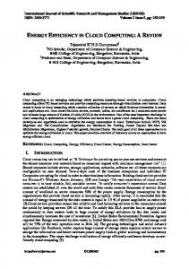
Figure 3: Comparison des valuers moyennes de di↵´erentes m´etriques (100 APs, 27 switchs avec 2 Gateways, taux d’arriv´ee des client dans le r´eseau `a 70 requˆetes/hour) d’´energie d’un lien n´egoci´e ` a 1Gbps est plus importante que la consommation d’´energie dans le cas d’un lien n´egoci´e ` a 10Mbps. Notons que cet algorithme d’adaptation des d´ebits des liens filaires est utilis´e par l’algorithme de reconfiguration pour calculer la consommation d’´energie au moment de la configuration. Pour ´evaluer les performances de notre approche, nous l’avons test´ee `a travers des simulations pour di↵´erentes configurations de r´eseaux et di↵´erentes charges de trafic dans le r´eseau. Grˆ ace ` a ces simulations, nous avons montr´e que notre approche propos´ee est capable de r´ealiser des gains significatifs en termes de consommation d’´energie, par rapport aux solutions de routage classiques telles que le routage par les plus courts chemins (Shortest Path, SP), le routage qui utilise la m´etrique de la plus petite capacit´e r´esiduelle des liens (Minimum Residual Capacity, MRC) et l’´equilibrage de charge (Load Balancing, LB). De plus, nous avons compar´ee notre approche avec celle bas´ee sur un algorithme heuristique vorace (Greedy-OFER) au lieu des colonies de fourmis (meta-heuristique). Quelques r´esultats de simulations sont montr´es dans la Figure 3. Plus pr´ecis´ement, nous montrons que notre approche permet de r´eduire la consommation d’´energie jusqu’`a 4%, 15%, 43% and 52%, par rapport `a Greedy-OFER, MRC, SP et LB, respectivement, tout en assurant la qualit´e de service (QoS) requise par les flux utilisateurs. Notons que cette contribution a fait l’objet de deux publications, une publication dans une conf´erence internationale (Globecom) [18] et une publication en cours de soumission dans le journal IEEE Transactions on Networks and Service Management (TNSM) [19].

3.3

Greenhead: Placement de data center virtuels (Virtual Data Centers) dans une infrastructure distribu´ ee de data centers

Le Cloud a r´ecemment gagn´e en popularit´e comme un mod`ele rentable pour l’h´ebergement de services en ligne ` a grande ´echelle dans de grands data centers. Dans un environnement de Cloud computing, un fournisseur d’infrastructure ou fournisseur Cloud (CP) partitionne les ressources physiques ` a l’int´erieur de chaque data center en ressources virtuelles (par exemple, les machines virtuelles (VM)) et les loue aux fournisseurs de services (SP) `a la demande. D’autre part, un fournisseur de services (SP) utilise ces ressources pour d´eployer ses applications et services, dans

3. Contributions

7

le but de les fournir ` a ses utilisateurs finaux `a travers l’Internet. Actuellement, les fournisseurs Cloud comme Amazon EC2 [20] o↵rent principalement ces ressources en termes de machines virtuelles sans fournir aucune garantie de performances en termes de bande passante et de d´elais de propagation entre les di↵´erentes machines virtuelles. L’absence de telles garanties peut a↵ecter de mani`ere significative les performances des services et applications d´eploy´es [21]. Pour rem´edier `a cette limitation, des propositions de recherche [22] et des o↵res Cloud [23] ont pr´econis´e d’o↵rir des ressources pour les fournisseurs de services sous la forme de data center virtuels ou Virtual Data Center (VDC). Un VDC est une collection de machines virtuelles, de switchs et routeurs virtuels reli´es entre eux par des liens virtuels. Chaque lien virtuel est caract´eris´e par sa capacit´e en bande passante et son d´elai de propagation. Par rapport ` a des o↵res de type machines virtuelles uniquement sans garanties de bandes passantes entre ces derni`eres, les VDCs sont en mesure de fournir une meilleure isolation des ressources du r´eseau, et ainsi am´eliorer les performances des applications et services. Malgr´e ses avantages, o↵rir un VDC comme un service pr´esente un nouveau d´efi pour les fournisseurs Cloud appel´es le probl`eme de VDC embedding (ou placement de VDC), qui vise `a placer les resources virtuelles (par exemple, machines virtuelles, les switchs, les routeurs) sur l’infrastructure physique. Jusqu’` a pr´esent, peu de travaux ont abord´e ce probl`eme [21, 24, 25]. Ces travaux ont consid´er´e uniquement le cas o` u toutes les composantes du VDC sont plac´ees dans le mˆeme data center. Il est ` a noter que ces o↵res en forme de VDC sont tr`es attractives pour les fournisseurs de services et les fournisseurs Cloud. En particulier, un fournisseur de services utilise son VDC pour d´eployer divers services qui fonctionnent ensemble afin de r´epondre aux demandes des utilisateurs finaux. Comme le montre la Figure 4, certains services peuvent exiger d’ˆetre dans la proximit´e des utilisateurs finaux (par exemple, les serveurs web) alors que d’autres peuvent ne pas avoir de telles contraintes de localisation et peuvent ˆetre plac´es dans n’importe quel data center (par exemple, les jobs MapReduce). D’autre part, les fournisseurs Cloud peuvent ´egalement b´en´eficier du placement de VDC dans leurs infrastructures distribu´ees. En particulier, ils peuvent profiter de l’abondance des ressources disponibles dans leurs data centers et d’atteindre divers objectifs, notamment maximiser les revenus, r´eduire les coˆ uts et r´eduire l’empreinte en carbone de leurs infrastructures. Dans cette troisi`eme contribution, nous proposons un framework capable d’orchestrer l’allocation de ressources aux VDC dans une infrastructure Cloud distribu´ee. Les principaux objectifs dans ce cas peuvent ˆetre r´esum´es comme suit: - Maximiser les revenus Certes, l’objectif ultime d’un fournisseur Cloud est d’augmenter son chi↵re d’a↵aires en maximisant la quantit´e de ressources allou´ees et le nombre de demandes de VDC satisfaites. Cependant, le placement des VDC n´ecessite la satisfaction de plusieurs contraintes, `a savoir la capacit´e et les contraintes de localisation g´eographiques. De toute ´evidence, le placement doit veiller ` a ce que la capacit´e de l’infrastructure physique ne soit jamais d´epass´ee. En outre, il doit satisfaire des contraintes de localisation des machines virtuelles impos´ees par les fournisseurs de services. - R´ eduire la charge du r´ eseau dans le r´ eseau backbone inter-data centers Pour faire face ` a la demande croissante du trafic entre les data centers, les fournisseurs d’infrastructures ont tendance ` a construire leur propre r´eseaux WAN de large ´echelle pour interconnecter leurs installations de data centers (par exemple, le r´eseau G-Scale de Google [26]). Dans ce contexte, l’un des objectifs cl´es du placement de VDCs est de minimiser le trafic dans le r´eseau backbone. En e↵et, il a ´et´e montr´e r´ecemment que le coˆ ut de construction d’un r´eseau d’interconnexion de data centers est beaucoup plus ´elev´e que le coˆ ut du r´eseau intra-data center, et il repr´esente 15%

3. Contributions

8

Figure 4: Exemple de delpoiment d’un VDC dans une infrastructure Cloud distribu´ee

du coˆ ut total de l’infrastructure [27]. En outre, selon plusieurs ´etudes [28], le r´eseau de transport inter-data center est le principal contributeur aux frais de transport de donn´ees. Par cons´equent, il est crucial de r´eduire le trafic r´eseau entre les data centers et placer les machines virtuelles qui ont besoin de communiquer beaucoup entre elles dans le mˆeme data center, `a chaque fois que cela est possible. - R´ eduire les coˆ uts op´ erationnels des data centers R´eduire les coˆ uts op´erationnels des data centers est un objectif principal de tout fournisseur Cloud puisque ceci impacte son budget de fonctionnement et sa croissance. Ceci peut ˆetre r´ealis´e en minimisant les coˆ uts de l’´energie, qui constitue une partie importante des d´epenses de fonctionnement total. Pour ce faire, deux techniques peuvent ˆetre adopt´ees: (1) mettre davantage de charge dans les data centers les plus ´econome en ´energie, et (2) profiter de la di↵´erence de prix de l’´electricit´e entre les emplacements des data centers pour utiliser les data centers qui pr´esente un prix d’´electricit´e minimal. De plus, les data centers ´economes en ´energie se distinguent par leurs Power Usage E↵ectiveness (PUE), qui donne le surplus d’´energie consomm´e par le data center pour refroidissements et d’autres fonctions annexes. Ainsi, les data centers `a faible PUE sont favoris´es pour accueillir plus de machines virtuelles. En outre, le fournisseur Cloud peut obtenir davantage d’´economies en tenant compte de la fluctuation des prix de l’´electricit´e au fil du temps et la di↵´erence de prix entre les emplacements des data centers. Par cons´equent, les machines virtuelles peuvent ˆetre efficacement plac´ees de telle sorte que le coˆ ut total de l’´electricit´e est minimis´e.

3. Contributions

9

Figure 5: Placement de VDCs dans une infrastructure Cloud distribu´ee

- R´ eduire l’empreinte en carbone Des recherches r´ecentes ont indiqu´e qu’en 2012, les ´emissions en carbone des data centers ` a travers le monde ont repr´esent´e 0, 25% des ´emissions en carbone dans le monde entier, ce qui repr´esente 10 % des ´emissions du secteur des TIC [29]. Par cons´equent, les fournisseurs Cloud sont confront´es ` a beaucoup de pression pour utiliser des sources d’´energie renouvelables (telles que l’´electricit´e g´en´er´ee par les ´eoliennes ou l’´energie solaire) pour rendre leurs infrastructures moins polluantes et respectueuses de l’environnement. Partant de ces observations, un placement efficace des VDCs devrait permettre de maximiser l’utilisation des ´energies renouvelables et de tenir compte de leurs disponibilit´e, ce qui d´epend de l’emplacement g´eographique du data center, la p´eriode de la journ´ee (par exemple, le jour pour l’´energie solaire) ainsi que les conditions m´et´eorologiques (par exemple, le vent, la pression atmosph´erique). En outre, chaque fois que l’´electricit´e du r´eseau ´electrique est utilis´ee, le fournisseur Cloud doit minimiser l’empreinte en carbone de son infrastructure. Dans ce cas, le placement des machines virtuelles est critique car l’empreinte en carbone par watt d’´electrict´e consomm´ee varie d’un endroit `a un autre. Dans ce contexte, nous proposons dans cette contribution Greenhead, un framework de gestion des ressources pour le placement des VDCs dans une infrastructure Cloud distribu´ee. Greenhead vise ` a maximiser les revenus du fournisseur Cloud en minimisant les coˆ uts d’´energie, tout en s’assurant que l’infrastructure est aussi respectueuse de l’environnement que possible. Greenhead op`ere en deux ´etapes. Nous partitionnons d’abord une requˆete VDC en plusieurs partitions telle que la demande en bande passante inter-partition est r´eduite au minimum et la bande passante intra-partition est maximis´ee. L’objectif de ce partitionnement est de mettre les machines virtuelles qui s’´echangent de gros volumes de donn´ees dans le mˆeme data center. Cela r´eduit consid´erablement le trafic achemin´e par le r´eseaux backbone d’interconnexion entre les data centers, et am´eliore ainsi le taux d’acceptation des requˆetes. Le partionnement du VDC

3. Contributions

10 1

0.8

0.6

0.4

0.2 Greenhead Baseline 0

io

e nc

pta

ce

Ac

rat

e tiv

t

ofi

pr

la

mu

Cu

e

on

kb

c Ba

k

or

tw ne

d

me

su

n Co

on er

st

les

ue

ati

liz uti

eq rr

pe

w po

of

a

iliz

Ut

n tio

re

on

int

st

ue

ab

w ne

eq rr

pe

r otp

fo

rb Ca

Figure 6: Comparison des valeurs moyennes de di↵´erentes m´etriques utilise une version modifi´ee de l’Algorithme de Louvain [30]. Par la suite, nous proposons un algorithme simple et efficace pour l’attribution des partitions aux data centers en fonction des contraintes g´eograpiques de certaines machines virtuelles, du prix de l’´electricit´e, du PUE de chaque data center, de la disponibilit´e des ´energies renouvelables et de l’empreinte en carbone par unit´e de d’´electricit´e dans les data centers. De mani`ere plus d´etaill´ee, l’architecture de Greenhead est illustr´e dans la Figure 5. Comme montr´e sur la figure, un fournisseur de services envoie sa requˆete de VDC au fournisseur Cloud, qui a la responsabilit´e d’allouer les ressources n´ecessaires. Naturellement, le fournisseur Cloud fera usage de son infrastructure distribu´ee avec l’objectif de maximiser son chi↵re d’a↵aires et r´eduire les coˆ uts d’´energie ainsi que l’empreinte en carbone. C’est l`a que Greenhead entre en sc`ene. Greenhead est compos´e de deux types d’entit´es de gestion: (1) un contrˆoleur central qui g`ere l’ensemble de l’infrastructure et (2) un contrˆoleur local d´eploy´e dans chaque data center pour g´erer les ressources internes du data center. L’entit´e centrale comprend cinq modules comme repr´esent´e dans la Figure 5: • Le module de partitionnement est responsable du partitionnement des VDCs de telle sorte que la bande passante inter-partition est r´eduite au minimum. L’objectif de ce module est de r´eduire le nombre de liens virtuels `a allouer entre les data centers. Chaque partition est cens´ee ˆetre enti`erement plac´ee dans un data center unique. • Le module de placement des partitions est responsable du placement des partitions dans les di↵´erents data centers en se basant sur sur des statistiques d’ex´ecution collect´ees par le module de monitoring. Il veille `a ce que toutes les partitions soient plac´ees tout en r´ealisant la rentabilit´e, l’efficacit´e ´energ´etique telle que la r´eduction des coˆ uts de l’´electricit´e du r´eseau ´electrique et de maximiser l’utilisation des sources d’´energie renouvelables. • Le module d’allocation de liens virtuels entre les data centers alloue les liens virtuels dans le r´eseau backbone qui interconnecte les data centers. Ces liens virtuels interconnectent les machines virtuelles qui ont ´et´e plac´ees dans di↵´erents data centers. • Le module de monitoring est responsable de la collecte des di↵´erentes statistiques des

3. Contributions

11

di↵´erents data centers. Les informations collect´ees incluent les PUE, l’utilisation des ressources, la temp´erature ext´erieure, le prix de l’´electricit´e et la quantit´e d’´energie renouvelable disponible. • La base de donn´ees des VDCs contient toutes les informations sur les VDC pr´esents dans le syst`eme, leurs partitions et la cartographie de leur placement dans les data centers et dans le r´eseau backbone d’interconnexion des data centers. Enfin, chaque contrˆ oleur local d’un data center a pour mission d’allouer les resources au partitions qui lui ont ´et´e attribu´ees par le contrˆoleur central. Pour montrer Greenhead en action, nous avons e↵ectu´e plusieurs simulations dans une infrastructure de 4 data centers dans 4 villes am´ericaines, interconnect´ees par le r´eseau NSFNet. Greenhead a ´et´e compar´e avec l’approche de base qui n’utilise pas de partionnement des VDCs. Nous avons mesur´e di↵´erentes metriques de performances telles que le taux d’acceptation des requˆetes VDC, le coˆ ut de consommation d’´electricit´e, l’utilisation de l’´energie renouvelable, l’empreinte en carbone et l’utilisation du r´eseau backbone inter-data center. Les r´esultats, comme pr´esent´es dans la Figure 6, montrent que Greenhead peut g´en´erer plus de revenue tout en minimisant les coˆ uts en ´electricit´e et les empreintes en carbone. Notons que cette contribution a fait l’objet d’une publication dans le journal IEEE Transactions on Cloud Computing [31].

3.4

Greenslater: Les Green SLAs dans les infrastructures Cloud distibu´ ees

Dans la contribution pr´ec´edente, nous nous sommes int´eress´es au cas du fournisseur Cloud qui souhaiterait r´eduire ses coˆ uts op´erationnels et ses empreintes en carbone tout en maximisant ses revenues, mais sans que le fournisseur de services n’intervienne sur les ´emissions en carbone des resources allou´ees ` a son VDC. Dans cette nouvelle contribution, nous nous int´eressons au cas o` u les fournisseurs de services qui utilisent les VDCs allou´es par le fournisseur Cloud, rajoutent des contraintes en termes d’emissions en cabone caus´ees par leurs VDCs. Les motivations de ce travail viennent de plusieurs ´etudes et rapports publi´es r´ecemment par di↵´erents organismes. En e↵et, avec l’augmentation de la consommation d’´energie et l’impact environnemental des infrastructures Cloud, le secteur des TIC connait un mouvement ascendant vers l’´ecologisation des infrastructures et des services Cloud. Ce movement est propuls´e d’un ˆot´e par des consid´erations de marketing et de l’autre par plusieurs r´eglementations gouvernementales. Par exemple, une ´etude r´ecente [32] a montr´e que la valeur des entreprises diminuerait de fa¸con significative si elles ont une empreinte en carbone ´elev´ee. Le mˆeme constat est fait, selon la mˆeme ´etude, pour les entreprises qui refusent de divulguer des informations sur leurs taux d’´emission en carbone. Par cons´equent, de nombreuses entreprises informatiques ont volontairement choisi de rendre publique leurs ´emissions en carbone et rendre compte r´eguli`erement de leurs e↵orts pour le d´eploiement de solutions et de services respectueux de l’environnement [33]. D’autre part, les gouvernements imposent des taxes sur les ´emissions en carbone dans l’espoir de pousser plus loin cette ´evolution vers l’adoption de sources d’´energie renouvelables et la r´eduction des ´emissions en carbone [34]. Par exemple, le gouvernement britannique exige que les entreprises consommant plus de 6 GWh d’´energie par ann´ee ach`etent des cr´edits de carbone [35]. De plus, certains gouvernements ont impos´e des taxes sur les ´emissions en carbone, dont le coˆ ut par tonne de CO2 ´emise est d’environ 30 Dollars [36]. Par cons´equent, ces taxes auront un impact financier sur les entreprises [34]. Dans le contexte du Cloud, les fournisseurs Cloud sont responsables de l’allocation des ressources pour les VDCs ` a travers leurs infrastructures Cloud distribu´ees dans le but de

3. Contributions

12

minimiser les coˆ uts d’exploitation et en essayant de respecter l’environnement en augmentant l’utilisation des ´energies renouvelables. Toutefois, r´ecemment, les fournisseurs de services ´etaient ´egalement tenus de prendre en compte les objectifs environnementaux et veiller `a ce que leurs services soient fournis avec des ´emissions en carbone r´eduites. Ainsi, de nombreux conseils consultatifs et commissions (par exemple, Open Data Center Alliance [37] et le SLA Expert Subgroup du Cloud Selected Industry Group de la commission europ´eene [38]) poussent vers la d´efinition des Green SLAs dans lesquels les fournisseurs de services exigent de leurs fournisseurs Cloud une limite sur les ´emissions en carbone g´en´er´ees pour h´eberger leurs services. Ceci s’est accompagn´e de propositions et de travaux de recherche. Par exemple, r´ecemment, des travaux de recherche ont pr´econis´e l’utilisation de ce type de SLA dans les Clouds de type High Performance Computing (HPC) [39–43]. Typiquement, les termes green des Green SLAs sp´ecifient soit des limites sur les ´emissions en carbone g´en´er´ees par le fournisseur Cloud pour h´eb´erger les services des fournisseurs de services [39–42], soit la quantit´e minimale d’´energie renouvelable ` a ˆetre consomm´ee par les ressources allou´ees au fournisseur de services [43]. Toutefois, ces propositions n’ont par abord´e le cas des VDCs, et ne tiennent donc pas compte de l’existence des demandes de bande passante (liens virtuels) et ne visent qu’`a allouer les machines virtuelles au sein d’un mˆeme data center. Dans ce contexte, nous avons ´etudi´e comment un fournisseur Cloud peut satisfaire les Green SLAs (i.e.; des SLAs avec des exigences green). En particulier, nous avons consid´er´e les Green SLAs qui sp´ecifient une limite sur les ´emissions en carbone g´en´er´ees par le VDC de chaque fournisseur de services. Pour cela, nous avons propos´e Greenslater, un framework qui orchestre l’approvisionnement et l’optimisation des ressources pour les multiples VDC h´eberg´es par le fournisseur Cloud dans une infrastructure distribu´ee. Du point de vue du fournisseur Cloud, l’objectif est de maximiser les revenus tout en minimisant les coˆ uts op´erationnels et les potentiels coˆ uts dus aux violations des termes des Green SLAs. Greenslater profite de la variabilit´e dans l’espace et dans le temps des ´energies renouvelables disponibles et les prix de l’´electricit´e dans les di↵´erents data centers. De plus, Greenslater utilise la reconfiguration dynamique pour optimiser dynamiquement l’allocation des ressources au fil du temps, tout en satisfaisant les contraintes des Green SLAs. L’architecture de Greenslater est similaire `a celle de Greenhead. En e↵et, Greeslater est compos´e de deux types d’entit´es de gestion: (1) un contrˆoleur central qui g`ere l’ensemble de l’infrastructure et (2) un contrˆoleur local d´eploy´e dans chaque data center pour g´erer ses ressources internes. Le contrˆ oleur central dispose en plus d’un module de migration dynamique de partitions. Le but ´etant de migrer des parties de VDC depuis les data centers qui n’ont pas d’´energie renouvelable disponible vers des data centers qui ont de l’´energie renouvelable disponible. Ainsi, les ´emissions en carbone sont r´eduites et les violations des Green SLAs sont minimis´ees, voire ´evit´ees. Greenslater utilise le mˆeme algorithme pour partitioner les VDCs en partitions dont les demandes en bandes passantes entre di↵´erentes partitions sont r´eduites. Par la suite, un algorithme heuristique pour placer les di↵´erentes partitions dans di↵´erents data centers est utilis´e. Comme la disponibilit´e des ´energies renouvelables dans les data centers ainsi que le prix de l’´electricit´e varient dans le temps, on utilise un algorithme de reconfiguration qui d´ecide de migrer des parties de VDC vers des data centers qui ont de l’´energie renouvelable disponible. Pour ´evaluer les performances de Greenslater, nous avons fait des simulations dans une infrastructure distribu´ee de 4 data centers interconnect´es par le biais du r´eseau NSFNet. Nous l’avons compar´e avec trois autres approches: (i) Greenhead [31], (ii) Greenhead sans partitionnement (NP) (i.e., chaque machine virtuelle d’un VDC est consid´er´ee comme ´etant une paritition), et (iii) l’approche Load Balancing (LB) [44]. Nous avons consid´er´e cinq metriques pour l’´evaluation:

4. Organisation de la th`ese

13

1

0.8

0.6

0.4 Greenslater Greenhead Greenhead NP Load Balancing

0.2

0 p

ce

Ac

o

ati

er

c tan

ve ati

l

mu

Cu

t

on ati

of

int

les

ofi

pr

tpr

ab

re

w ne

o

rb

Ca

oo nf

ion

lat

A

SL

vio

iliz

Ut

Figure 7: Comparaison des valeurs cumulatives de di↵´erentes m´etriques (i) le profit empoch´e par le fournisseur Cloud, qui est la di↵´erence entre les revenues et la somme des coˆ uts d’exploitation (c’est-` a-dire les coˆ uts de l’´energie, le r´eseau d’interconnexion des data centers et les coˆ uts de violation des Green SLAs), (ii) le taux d’acceptation (d´efini comme le rapport des requˆetes accept´ees sur un total des requˆetes), (iii) l’empreinte en carbone g´en´er´ee par l’ensemble de l’infrastructure, (iv) l’utilisation de l’´energie renouvelable et (v) les violations des Green SLA. Quelques r´esultats sont donn´es par la Figure 7. Ces r´esultats montrent que Greenslater permet toujours d’obtenir des profits plus ´elev´es, assure une plus grande utilisation des ´energies renouvelables et moins d’´emissions en carbone avec un minimum de violations des Green SLAs. Par exemple, le gain en termes de profit donn´e par Greenslater est d’environ 33%, 53% et 120%, par rapport ` a Greenhead, Greenhead NP et l’approche de Load Balancing, respectivement. Notons que cette contribution a fait l’objet d’une publication dans la conf´erence internationale CNSM [45].

4

Organisation de la th` ese

Le reste de cette th`ese est organis´e en deux parties. La premi`ere partie traite la r´eduction de la consommation d’´energie dans les r´eseaux d’acc`es sans fil et les r´eseaux de campus. On commence dans un premier temps par un ´etat de l’art d´etaill´e des travaux autours de cette th´ematique. Puis nous pr´esentons dans les deux chapitres suivants nos contributions dans les r´eseaux sans fil multi-saut et les r´eseaux de campus. La deuxi`eme partie de la th`ese traite la r´eduction de la consommation d’´energie et les ´emissions en carbone des infrastructures Cloud. Comme pour la premi`ere partie, nous nous int´eressons `a l’´etat de l’art autours de cette th´ematique. Puis nous d´ecrivons nos deux contributions dans les deux chapitres suivants qui consistent en la r´eduction de la consommation d’´energie, l’exploitation des energies renouvelables disponibles et la r´eduction des ´emissions en carbone dans les infrastructures Cloud distribu´ees, dans deux contextes di↵´erents: le cas d’un founisseur Cloud qui veut r´eduire ses coˆ uts et le cas o` u les clients du fournisseur Cloud demandent des garanties sur les ´emissions en carbone de leurs services h´eberg´es dans le Cloud.

Chapter 1

Introduction 1.1

Context and Motivations

Over the last few years, the Information and Communication Technologies (ICT) became a considerable power consumer and polluter. In fact, the ICT sector consumes alone 3% of world wide energy consumption, and its CO2 emission was around 2% in 2010. This is equivalent to airplanes emission and a quarter of cars emissions [1]. Moreover, according to a recent report posted online by the CEO of Digital Power Group Mark Mills [2], the ICT ecosystem, which includes the cloud as well as the digital devices and wireless networks that access its services, is approaching 10% of the world’s electricity usage. Furthermore, the updated analysis of the SMART 2020 report [3] shows the relative shift in the energy footprint of the ICT sector from devices to data center and networks. In fact, networks and data center will account each of them for 25% of the power ICT consumption [3,4]. This increase in energy consumption is mainly due to the widespread availability of wireless broadband access and the massive migration towards the cloud for service provisioning. Indeed, over the last decade, there has been an increasing use of personal wireless communications devices, such as smartphones and tablets. This trend is pushing faster and harder the wireless cloud (i.e., cloud services consumed though wireless devices) [5, 6]. In fact, the traffic of wireless cloud is increasing by 95% every year [5, 6]. Consequently, the amount of consumed power in the access networks is expected to soar as a significant amount of power is consumed by the transport of data when traffic is exchanged between a service provider and the end users [46]. Specifically, according to a study published in 2013 [6], the wireless cloud services energy consumption, in which wireless access networks represent 90%, will increase by 460% in 2015 to reach 43 TWh, up from 9.2 TWh only in 2012. According to this same study, this will result is an increase in its carbon footprint from 6 megatonnes of CO2 in 2012 to up to 30 megatonnes in 2015, which represents the equivalent of adding 4.9 million cars to the roads. These services are supported by data storage and processing infrastructure (commonly referred to as the cloud) located in large data centers spread around the globe. According to a report published by Greenpeace in 2013 [4], if the cloud was a country, it would have the sixth highest power consumption in the world. Furthermore, data centers energy demand alone grew to an estimated 40GW in 2013, an increase of 7% over 2012 [7]. This number is expected to increase significantly by 2020 [3]. To make the matter worse, this high power consumption is accompanied by high carbon emission as the dominant source for power generation rely on non renewable sources [8, 9]. In light of this, energy efficient networking and green clouds are becoming an important 14

1.2. Contributions

15

research direction among the research community and ICT industry. In fact, several studies have shown keenness to reduce energy consumption and carbon emissions from ICT companies [10–13]. The main objective is to reduce operational costs and achieve social corporate responsibility. As such, energy efficient infrastructures have emerged as a promising solution to achieve sustainable and cost e↵ective operations of access networks and cloud infrastructures. In this context, this thesis addresses the problem of building and running green and energy efficient infrastructures. We focus on cloud infrastructures, from access networks to core data centers. More specifically, we first address the energy reduction in wireless access networks and campus networks. Then, we present a framework for energy efficient and green distributed cloud infrastructure. In what follows, we summarize the di↵erent contributions in Section 1.2. Then, we present the organization of this thesis in Section 1.3.

1.2

Contributions

In this thesis, we addressed two major challenges in mobile cloud infrastructures. Specifically, we present four contributions for energy efficient and green infrastructures, in both access networks and distributed cloud infrastructures. The first contribution addresses the energy reduction in TDMA multihop wireless networks. The second contribution extends the energy efficiency to the scale of a campus network. Then, the last two contributions addressed the energy efficiency and green infrastructures in distributed clouds. More specifically, we first address the problem of reducing energy consumption, costs and carbon footprint in distributed clouds. Then, we extend the problem to o↵er Green SLAs, through dynamic reconfiguration. In what follows, we present in a nutshell these contributions.

1.2.1

Green Routing and Link Scheduling in TDMA-based Multihop Networks

As a first contribution, we propose an energy-efficient framework for joint routing and link scheduling in multihop TDMA-based wireless networks. Our objective is to find an optimal tradeo↵ between the achieved network throughput and energy consumption. To do so, we first propose an Optimal approach, called Optimal Green Routing and Link Scheduling (OGRLS), by formulating the problem as an integer linear program (ILP). As this problem is N P-Hard, we then propose a simple yet efficient heuristic algorithm based on Ant Colony, called AC-GRLS. Through extensive simulations, we show that both approaches can achieve significant gains in terms of energy consumption, flow acceptance ratio and achieved throughput, compared to the Shortest Path (SP) routing, and the Minimum link Residual Capacity (MRC) based routing. This contribution is the object of a conference publication in the International Conference on Network and System Management (CNSM) [14] and a journal publication in Computer Networks [15].

1.2.2

Online flow-based management for energy efficient campus networks

As a second contribution, we propose a flow-based management framework to achieve energy efficiency in campus networks. Typically, a campus network is composed of a wireless part mainly Access Points (APs) and a copper based backbone network made up by layers of switches. We address the problem from the dynamic perspective, in that users come and leave the system in unpredictable way. This is new compared to the previous contribution where traffic and users are assumed to be known and fixed in advance at the planning stage. Specifically, we propose

1.3. Outline

16

an online flow-based routing approach, that allows dynamic reconfiguration of existing flows as well as dynamic link rate adaptation, while taking into account users’ demands and mobility. Our approach is compliant with the emerging Software Defined Networking (SDN) paradigm since it can be integrated as an application on top of an SDN controller. To achieve this, we first formulate the flow-based routing problem as an integer linear program (ILP). As this problem is known to be N P-hard, we then propose a simple yet efficient Ant Colony-based approach to solve the formulated ILP. Through extensive simulations, we show that our proposed approach is able to achieve significant gains in terms of energy consumption, compared to a heuristic solution, conventional routing solutions such as the Shortest Path routing (SP), the Minimum link Residual Capacity routing metric (MRC) and the load balancing (LB) scheme. Note that this contribution is the object of a conference publication in the the Global Communication conference (Globecom) [18] and the forthcoming publication [19].

1.2.3

Greenhead: Virtual Data Center Embedding Across Distributed Infrastructures

In the second part of our research, we propose Greenhead, a holistic resource management framework for embedding Virtual Data Centers (VDCs) (i.e., a set of virtual machines and virtual links with guaranteed bandwidth) across geographically distributed data centers connected through a backbone network. The goal of Greenhead is to maximize the cloud provider’s (CP) revenue while ensuring that the infrastructure is as environment-friendly as possible. To do so, we first divide a VDC request into partitions such that the inter-partition bandwidth demand is minimized. Then, we propose an efficient algorithm for assigning partitions to data centers based on energy cost and carbon footprint metrics. To evaluate the e↵ectiveness of our proposal, we conducted extensive simulations of four data centers connected through the NSFNet topology. Note that this contribution is the object of a journal publication in Transactions on Cloud Computing (TCC) [31].

1.2.4

Greenslater: Providing green SLA in distributed clouds

In the last part of this dissertation, we provide a solution for how can cloud providers meet Service Level Agreements (SLAs) with green requirements. In such SLAs, an SP requires from CPs that carbon emissions generated by the leased resources should not exceed a fixed bound. To do so, we propose Greenslater, a resource management framework allowing a CP to provision resources in the form of VDCs across a geo-distributed infrastructure with the aim of reducing operational costs and green SLA violation penalties. Through extensive simulations, we show that the proposed solution maximizes the cloud provider’s profit and minimizes the violation of green SLAs. Note that this contribution is the object of a publication in the International Conference on Network and Service management (CNSM) [45].

1.3

Outline

This thesis is organized into two parts. The first part addresses the energy reduction in wireless mesh and campus networks. In view of this, we first present in Chapter 2 relevant related work dealing with energy reduction in wired networks, wireless local area networks (WLANs), campus networks, wireless mesh networks (WMNs), and cellular networks. Then, we present, respectively, in Chapter 3 and Chapter 4, our

1.3. Outline

17

first two contributions, namely, Green Routing and Link Scheduling in TDMA-based Multihop Wireless Networks, and Online flow-based Routing for Energy Efficient Campus Networks. In the second part, we address the problem of running green cloud infrastructures. More specifically, we first present in chapter 5 the state of the art regarding green and energy reduction in clouds. Specifically, we start by highlighting the motivations towards greening the cloud infrastructures. Then, we present relevant work dealing with energy reduction inside a single data center, across multiple data centers, and virtual network embedding and mapping. Finally, a presentation of green service level agreements in the Cloud concludes the chapter. The, we present our two contributions in Chapter 6 and Chapter 7, respectively. Specifically, Chapter 6 presents Greenhead, our third contribution focusing on reducing the energy costs and carbon footprints of a distributed cloud infrastructure under a best e↵ort case. Chapter 7 investigates how can Cloud Providers meet Green SLAs by presenting our last contribution Greenslater, which aims to embed VDCs across distributed cloud infrastructure under explicit green constraints. Finally, Chapter 8 concludes this thesis and presents a perspective for future work.

Part I

Energy Efficiency in Access Networks

18

Chapter 2

Energy Reduction in Wireless and Wired Networks: State of the Art 2.1

Introduction

Energy management has been an active research area in the last few years. A plethora of works addressed this problem in di↵erent types of networks, at di↵erent scales (small, medium and large networks) and for di↵erent technologies (wireless, copper and optical networks). The proposed approaches aim at reducing the network power consumption by using smart on/o↵ techniques. Indeed, access and core networks are designed to handle peak surges of traffic. As such, during low traffic periods, parts of the network are under-utilized, and yet consume a considerable amount of energy. In this chapter, we summarize existing works on reducing energy consumption in wireless and wired networks. For the sake of presentation, we organize these works according to the type of network under study. We first start by the wireless LANs and campus networks in Section 2.2, followed by Wireless Mesh Networks (WMNs) in Section 2.3. Energy reduction in cellular networks is presented in section 2.4. Section 2.5 presents relevant works dealing with energy reduction in wired networks. Section 2.6 discusses these works and positions our contributions in this research area. Finally, Section 2.7 concludes this chapter.

2.2

Energy Reduction in WLANs and Campus Networks

A WLAN or campus network is typically composed of a set of Access Points (APs) deployed in an enterprise or university campuses. These APs are connected to layers of switches that compose the access, aggregation and core enterprise network. The APs serve the mobile users and use the layers of switches in the network to provide connectivity to the Internet through core router gateways. These networks drain a considerable amount of power as they are designed to handle peak traffic demands. As such, in low traffic demand, parts of the network are not used or underutilized, which results in power wastage. To address this problem, existing works in the literature proposed energy efficient techniques to reduce the amount of consumed power. For instance, authors in [47] presented strategies based on the resource on-demand concept. The idea is to power on/o↵ WLAN APs dynamically, based on the volume and location of user demand in a high-density WLANs (i.e., redundant coverage and connectivity in the network). More specifically, authors proposed SEAR (Survey, Evaluate, Adapt, and Repeat), which uses online measurement of the resource consumption in the network 19

2.3. Energy Reduction in WMNs

20

and user traffic estimation to provide the minimum number of nodes in the network to be used to accommodate the traffic load. As such, users traffic is drained with the required QoS and with a minimum power consumption. SEAR relies on a central controller for information collecting and decision making. More specifically, it uses a clustering algorithm to group the APs that are close to each other. Then, through demand estimation of users’ traffic, a number of APs to be turned on is selected to match the traffic demand. In the same context as [47], authors in [48, 49] proposed an analytical model to assess the e↵ectiveness of policies that activate APs in dense WLANs, according to users’ demands and QoS requirements. This model assumes dense WLANs with a centralized controller. A clustering algorithm groups the APs in close proximity of each other, and the proposed model focuses on the behavior inside a single cluster. More specifically, they model user association to APs policies where the number of APs to switch on is defined by the number of associated users to APs of the same cluster. The number of APs is defined using predefined thresholds. The authors also propose a traffic-based policy model, which uses the amount of traffic received by the APs instead of the number of associated users. From a practical implementation point of view, some works evaluated the impact on a production network. For instance, authors in [50] evaluated the implementation of the Resource on Demand policies proposed in [48] in a student study room of Politecnico di Torino (PoliTo). Their results confirm energy saving in a campus WLAN environment, depending on the times of the day, the days of the week, and the period of the year. From the industry perspective, solutions that integrate energy management in WLAN infrastructures exist. For instance, cisco EnergyWise solutions [51] propose to set up predefined profiles for network nodes. The profiles contain periods of operation/sleep of the nodes. As such, parts of the network are switched o↵ in times of non-utilization such as night times in corporate buildings, to reduce the energy consumption.

2.3

Energy Reduction in WMNs

In the context of Wireless Mesh Networks (WMNs), classical routing and link scheduling algorithms focus on the performance in terms of network throughput and delay. A survey of some of the existing works in literature is presented in [52]. However, these works did not address the energy consumption issue. Recently, energy consumption in WMNs has gained importance. The most relevant works on energy efficiency are reported in [53–59]. Specifically, authors in [53] propose to reduce energy consumption in wireless-optical broadband access networks (WOBAN) by reducing the number of used optical and mesh nodes. In WOBAN, end-users receive broadband services through a WMN, which is connected to an optical backbone network via gateway nodes. Authors formulate the problem as mixed integer linear program (MILP) model for multi commodity flow and provide the optimal routing to reduce the number of used nodes. The objective is to reduce the number of optical nodes to use in the backbone network. The traffic in the wireless part of the network (WMN) is routed using the minimum residual capacity as a routing metric, which aims at consolidating the traffic into a reduced number of nodes in the network. In [54], the authors considered the case of WMNs where the clients can choose the AP they connect to. To do so, they formulate the problem as an ILP, where the objective is to minimize the number of used nodes (APs and gateways), while the demand is always satisfied. This work was extended in [55] to include the cost of nodes’ deployment. In the latter work, the objective is to choose between the energy cost (OpEx) and the deployment cost (CapEx) of a WMN.

2.4. Energy Reduction in Cellular Networks

21

However, in these two works, the authors did not take into account the interference between APs since directional antennas are assumed. In addition, they focus only on optimizing energy consumption without addressing the network throughput issue. Another energy management study in WMNs is provided in [56], where a combination between di↵erent modulation techniques and power adaptation is presented and column generation is used to solve the problem. Authors in [58] present an energy and throughput-aware routing protocol in WMNs. The proposed algorithm admits as many flows as possible while satisfying their throughput demands, and at the same time uses as few nodes as possible by switching o↵ the unused ones. The problem was formulated as a multi-commodity flow problem. However, the authors assume a pre-established channel assignment in WMNs in order to avoid undesired interferences. As such, the proposed routing protocol targets only 802.11-based networks. Authors in [59] proposed an approach for video delivery in battery operated WMNs. The context of battery operated WMNs is similar to Wireless Sensor Networks where the energy supply is limited at each node and is in constant decrease. However, the di↵erence in WMNs is that users are mobile, which adds more constraints and challenges. Their proposed approach seeks a balance between the energy saving and network delivery performance and user perceived quality. More specifically, it consists of a MAC layer mesh point operation cycle management scheme, which controls the sleep pattern of APs, and a routing metric that integrates the remaining energy, distance to the destination and traffic load of each node along the path. This defined metric is used in an extension of the OLSR routing protocol [60]. To address the problem of designing and operating green WMNs, authors in [57, 61] investigated the possibility of using renewable energy to power WMNs. The objective is to make use of the available renewable energy to satisfy the QoS of the traffic carried in the network. As such, the fundamental design criterion and main performance metric have shifted from energy efficiency to energy sustainability. Consequently, the authors’ proposals aimed at ensuring traffic routing in the network using the dynamically harvested green power. To this end, authors first addressed in [57] the placement problem of green access points (i.e., APs powered by sustainable energy sources) to meet users’ QoS demand, followed by a resource management scheme to address the unreliability of renewable energy. Recently, they proposed in [61] a queuing theory model for the energy bu↵er in a WMN, and proposed a resource management scheme that balances the traffic in the network based on the available renewable energy at the mesh nodes. Their proposed approach further includes a distributed admission control at the mesh APs level to seek a trade-o↵ between resource utilization and quality of service provisioning, which literally means limiting the number of users in the network to guarantee the QoS under the intermittent availability of renewable power. In the same context of operating sustainable WMNs, authors in [62] addressed the problem of green relay nodes deployment (i.e., relay nodes operated by renewable power) and subcarrier allocation. They first formulated the problem as a non-linear programming problem and proposed two heuristic algorithms to solve it.

2.4

Energy Reduction in Cellular Networks

Similar to WMNs and WLANs, cellular networks are designed to handle peak traffic demands, with cell towers covering significant geographic areas. As such, solutions that aim at reducing the energy consumption of such networks by shutting down unused cells have been proposed. Some proposals in this direction are [63, 64]. In view of this, authors in [63] present an analytical model energy-aware management of cellular access networks, where the objective is to characterize the potential energy saving by reducing the number of active cells during periods

2.5. Energy Reduction in Wired Networks

22

of low traffic. Similarly, authors in [64] investigate energy saving procedures by turning o↵ both transmission components during signal-free symbols and cells during low traffic periods. In fact, such control is more fine-grained compared to the previous approach and results in additional energy saving in this particular case of cellular networks, where the transmission component consume a considerable amount of power. In [65], the authors propose a framework for green communications in wireless heterogeneous networks. A heterogenous network is mainly composed of small cells and macrocells. This framework is cognitive in the holistic sense and aims at improving energy efficiency of the whole system, rather than one isolated part of the network. In the same context, authors in [66] investigated the design and the associated tradeo↵s of energy efficient cellular networks through the deployment of sleeping strategies (i.e., switching o↵ unused base stations) and use small cells, which are less power hungry, to o✏oad the macrocells. Moreover, authors in [67] provide a baseline for the potential of energy saving in cellular networks, by a combination of macro and femtocells. The objective is to find the set of base stations (BSs) to turn on in order to insure an entire coverage and minimize the energy. They presented a heuristic that identifies the BSs that are more likely to have clients and turn them on, and BSs that are more likely not to have clients and shut them down. Additional works on reducing the energy consumption in cellular networks are summarized in [68, 69].

2.5

Energy Reduction in Wired Networks

Numerous proposals have been presented to reduce energy consumption in wired networks [53, 70–80].These works aim at reducing the energy consumption by mainly switching o↵ unused nodes in the network, under low traffic demands, and adapt the links’ rates to adjust to the network demand. Orgerie et al. [81] proposed to use bandwidth reservation requests to plan network resources and reduce the number of used nodes in dedicated networks (e.g., across banks network). Their proposed solution aims at reducing the number of used nodes in the network, by having an end-toend control over the network. The proposed framework exploits the energy consumption profiles of the nodes in the network, the bandwidth reservation requests, the available bandwidth over the links in a centralized manner, and schedules the flows through computed paths. Moreover, authors use rate adaptation in the network to adjust the transmission rate of links to the actual load, to further achieve energy reduction. In the context of ISP core networks, authors in [70] proposed an approach to reduce the number of used nodes and links in a core network. Their proposal tries to shut down nodes one by one and verify that the network still routes the required traffic (i.e., the constraints are not violated). The same authors discussed a specific case study of wired backbone networks in [71], and presented an overall energy saving in the Internet scale in [72]. Authors in [77] proposed a solution that is time-driven and relies on the observation that ISP networks exhibit regular/predictive traffic patterns during specified time windows. Hence, they first propose a heuristic that shuts down unnecessary links, and then an algorithm to compute the duration of the time window. This approach is shown to be able to achieve up to 18% energy saving (in terms of used links) without significantly impacting the network performance. In [73], authors investigated a model based on gradient optimization to reduce energy consumption in wired networks. They started from routing paths given by a shortest path routing. Then, they used a routing policy named Energy-Aware Routing Protocol (EARP) [74], which switches o↵ some nodes in the network and re-routes the flows that are routed through these

2.6. Discussion

23

nodes. Their approach helps to reduce the energy consumption by up to 10% given that the required QoS is satisfied. Online flow-based routing also has been used in [75]. In an online approach, flows are assumed to come and leave the system in a dynamic way. Authors in [75] presented E2 -MCRA, a flow-based routing approach that reduces the number of used nodes in an ISP network, while satisfying the QoS constraints. The idea is to route incoming flows by choosing among the possible paths, the one that achieves the best combination between the path length and the number of additional nodes to turn on. Their path search strategy is based on Depth-Firth Search. Regarding decency on the physical cabling, authors in [76] target the specific bundled wired backbone networks. In a bundled backbone network, each link is composed of a set of aggregated cables. Their solution proposes to reduce the number of used cables in a link, while assuring the bandwidth demands of the flows using that link. Their approache starts from a configuration where all the cables are turned on. Then, they use a heuristic to select which cable to turn o↵ without altering the QoS of routed flows.

2.6

Discussion

In our study, we focus on WMNs and campus networks, two popular networks, providing last few miles last few hops connectivity. The particularity of these networks is that the traffic patterns are dynamic, and the load is variable over time. In this context, we propose a routing and link scheduling approach for traffic flows, in a centralized manner, which is suitable for the emerging SDN paradigm. We first focus on TDMA-based wireless multihop networks since TDMA-based channel access facilitates the use of Quality of Service (QoS)-aware link scheduling and routing [82,83]. Indeed, while the IEEE 802.11 protocol is the de facto standard for multihop wireless networks, its MAC protocol (Carrier Sense Multiple Access with Collision Avoidance, CSMA/CA) performs poorly in WMNs and it is almost impossible to guarantee QoS [83, 84]. To guarantee QoS, packet collisions must be avoided by scheduling interfering links to transmit in non-overlapping frequency or time intervals [83]. This is why several developments were provided using multihop MAC protocols based on TDMA, such as the IEEE 802.16 mesh protocol (e.g., WiMAX) [85], the 802.11s mesh deterministic access (MDA) protocol [86], and the software-based 802.11 overlay TDMA MAC protocol [83]. In this context, novel green and energy efficient routing and link scheduling strategies are needed to take into account energy consumption of wireless nodes when powered on. In this case, important questions arise: how many APs need to be active to route a traffic within a WMN and what is the optimal tradeo↵ between the achieved network throughput and energy consumption? To answer these questions, we first propose in the next chapter a holistic management framework that provides the WMN administrator with a parameterized objective function to achieve the desired trade-o↵ between network throughput and energy consumption. Our proposed approach takes explicitly into account the interference in a wireless environment, as opposed to existing schemes such as [53–55]. In addition, we focus on reducing the energy consumption by reducing the used nodes in the network, as opposed to approaches that focus on transmission power adaptation such as the ones listed in [87]. Moreover, online approaches for flow routing and dynamic reconfiguration have not been well studied in the literature. To fill this gap, we propose in Chapter 4, a new scheme that takes into account a dynamic scenario, where traffic patterns are not stable over time, and users’ arrivals

2.7. Conclusion

24

and departure are dynamic and unpredictable. Last but not least, our proposed approaches rely on meta-heuristics to find a near optimal solution in a reasonable time compared to brute force exhaustive search for the optimal solution. This makes our schemes more scalable and applicable in practice.

2.7

Conclusion

With the increasing demand for power in access networks, energy efficient solutions for network design and management are required based on the used technology, density and network load. In this chapter, we presented the most relevant works dealing with energy reduction in wireless and wired networks. In particular, we presented existing approaches related to WLANs, WMNs, cellular networks and wired networks. We then positioned our contributions in this research area. In the following two chapters, we detail our proposed approaches for reducing the energy consumption in TDMA-based wireless multihop networks and campus networks.

Chapter 3

Energy Efficient TDMA-based Wireless Mesh Networks 3.1

Introduction

The application of green networking to multihop wireless networks, in particular Wireless Mesh Networks (WMN), has seldom been reported in the literature. Typically, a WMN [88] comprises wireless mesh routers, also called access points (APs). Each AP serves multiple mobile users and connects them through multihop wireless routing to the wired network. The mesh nodes connected directly to the wired network (i.e., connecting the WMN to the wired network) are called gateways. They represent, respectively, the sources and sinks of downlink and uplink traffic in the WMN. Since such networks are expected to proliferate in the next few years, their energy consumption will impact the overall energy consumption of the Internet [89]. In this chapter, we focus on TDMA-based wireless multihop networks since TDMA-based channel access facilitates the use of QoS-aware link scheduling and routing [82, 83]. In this context, important questions arise: how many APs need to be active to route a traffic within a WMN and what is the optimal trade-o↵ between the achieved network throughput and energy consumption. To answer these questions, we propose in this chapter a holistic management framework that provides the WMN administrator with a parameterized objective function to achieve the desired tradeo↵ between network throughput and energy consumption. Specifically, we propose two methods: (i) an optimal one, called Optimal Green Routing and Link Scheduling (O-GRLS), and (ii) an heuristic one, called Ant Colony Green Routing and Link Scheduling (AC-GRLS). The reminder of this chapter is organized as follows. Section 3.2 presents the system model and the problem statement. Section 3.3 describes our proposed framework for energy management through green joint routing and link scheduling. First, we introduce the O-GRLS method, then we present the AC-GRLS algorithm. Simulation results are presented in Section 3.4. Finally, Section 3.5 concludes this chapter.

3.2

System Model

3.2.1

Network Model

We represent a WMN by a directed graph G(V, E), called a connectivity graph, where V = {v1 , ..., vn } is the set of n nodes and E is the set of possible direct communication links. Each 25

3.2. System Model

26

node vi 2 V represents an AP with a circular transmission range Rt (i) and an interference range RI (i). Among the set V of all wireless nodes, some of them are gateways, that provide the connectivity to the Internet. For simplicity, let S = {s1 , s2 , ..., sm } be the set of m gateway nodes, where si is the node vn+i m , for 1  i  m. All other wireless nodes vi (1  i  n m) 2 V \S are ordinary mesh nodes. Each ordinary mesh node will receive the traffic from all its attached users and then route it to the Internet through some gateway nodes. We assume that each node vi 2 V has a limited capacity to serve its attached clients, denoted by Ci , whereas the capacity between any gateway node to the Internet (to forward its incoming traffic to the Internet) is sufficiently large. During the transmission of the node vi 2 V , all the nodes residing in its transmission range, and thus representing its neighborhood denoted by Ne (i), receive the signal from vi with a power strength such that correct decoding is possible with high probability. A unidirectional wireless link exists between vi and every neighbor vj 2 Ne (i) and is represented by the directed edge (i, j) 2 E. Each link (i, j) contains a certain number of orthogonal channels, denoted by ncij . The capacity along each channel k (1  k  ncij ) is limited and denoted by Cijk . We represent the connectivity graph G(V, E) by a connectivity matrix, denoted by M . The connectivity matrix M is a matrix with rows and columns labeled by the graph vertices V , with a 1 or 0 in position (i, j) according to whether vi and vj are directly connected or not. Having the same structure, the number of channels in each link is modeled by a channel matrix, denoted by N C. If there is no direct link between i and j, then ncij = 0, and hence Cijk = 0.

3.2.2

Interference Model

In this chapter, we adopt the protocol interference model [52]. In this model, a node vj is interfered by the signal from vi whenever ||vi vj ||  RI (i) and vj is not the intended receiver. Recall that ||vi vj || (denoted also by dij for simplicity) refers to the Euclidean distance between vi and vj . To schedule two links at the same time slot, we must ensure that the scheduler will avoid the link interference. In other words, the transmission from vi to vj is viewed successful if ||vk vj || > RI (k) for every node vk transmitting in the same time slot on the same channel m (i.e., the receiver is interference free, as in [52]). Recall that the channels are assumed to be orthogonal. Hence, non-interfering links as well as interfering links operating on di↵erent channels can transmit in parallel during the same time slot. Note however that no simultaneous transmission and reception is allowed on the same node. Given a connectivity graph G(V, E), we use the conflict graph FG to represent the interference in G. Each vertex of FG corresponds to a directed link (i, j) in the connectivity graph G. There is a directed edge from vertex (i, j) to vertex (p, q) in FG if and only if the transmission of link (i, j) on channel m interferes with the reception of the receiving node of link (p, q) on the same channel. The conflict graph FG is then fully defined by the interference matrix I as follows: ⇢ 1 If (p, q) interferes with (i, j) I(i,j),(p,q) = 0 Otherwise.

3.2.3

AP Energy Consumption Model

In this work, an AP can be in three di↵erent states: Active(i.e., Transmitting/Receiving), Idle and OFF. Note that in the Idle state, an AP is ON, but is neither transmitting not receiving. As reported through the experimental measurements in [90], the power consumption of an Active

3.2. System Model

27

AP represents the peak power consumption, and an Idle AP consumes almost 75% of its peak power consumption. Finally, an OFF AP does not consume any power. As a result, we derive the following power consumption model for the power consumption Pi of an AP i as follows: 8 < 100% If AP i is Active 75% If AP i is Idle Pi = : 0% Otherwise.

3.2.4

Traffic Model

In our study, we consider a set L of mesh users (also called clients). Each user l 2 L generates a certain traffic demand dl (in terms of required bandwidth). To represent the user position within the WMN, we define a binary variable al,j to indicate whether a user l is within the coverage area of the AP j or not. Note that a user l can be within the coverage area of multiple APs. Our aim is to turn o↵ unnecessary APs to save energy, while achieving the required bandwidth of user l. The traffic demands of APs can follow a uniform distribution (i.e., each AP has the same demand) or a random process (e.g., Poisson process). According to [91], this traffic is assumed not to change during a given time interval. Indeed, in [91], the characteristics of the traffic in wireless access networks have been analyzed and it is shown that the traffic during the day can be divided into intervals of equal length. In particular, 8 intervals of 3 hours are defined, as in [54]. In this chapter, we adopt such characteristics. Without loss of generality, we assume that the traffic is uplink. This means that each originated traffic must be routed towards a gateway.

3.2.5

Problem Formulation

The general problem we are considering aims at managing mesh nodes in order to save energy when some of the network resources (i.e., APs including gateways and the links connecting them) are not necessary and can be switched o↵, while achieving the required user’s bandwidth. From an operational point of view, this can be easily integrated in network management platforms commonly used for carrier grade WMNs and to the centralized and remote control of all configured devices. As we consider a slotted, synchronized WMN, and a static topology and demands (within one interval of 3 hours, as stated in Subsection 2.4), it is reasonable to assume that the network is periodic with period T (i.e., each interval of 3 hours is divided into a number of periods of length T , where the length is measured in time slots). For instance, using WiMAX, the scheduling period T corresponds to the frame duration which is 5 20 ms long [92]. As stated earlier, we jointly consider green routing and link scheduling. Recall that a link scheduling consists in allocating to each link a set of time slots ⇢ {1, .., T } on which it will transmit. Our objective is to maximize both the total network throughput and energy saving by switching o↵ unused nodes. The throughput is given by the ratio of successfully routed traffic towards the gateways to the number of needed time slots. Hence, maximizing the throughput boils down to minimizing the total number of used slots within the scheduling period T . The problem can be thus described mathematically within a WMN, as follows: GIVEN: • A physical topology represented by the graph G(V, E), which is described by the connectivity, interference and channel matrices M , I and N C, respectively.

3.3. A Framework for Energy Efficient Management in TDMA-based WMNs

28

• A list L of clients, each one with its demand dl . • The coverage matrix A of APs, defined by the binary variable al,j . FIND: • The optimal attachment of each client among L to one of the covering APs and the optimal routing and link scheduling of its corresponding flow (traffic) that makes the best tradeo↵ between achieved network throughput and energy consumption. In what follows, we present our proposed framework to achieve this goal.

3.3

A Framework for Energy Efficient Management in TDMAbased WMNs

Our framework jointly considers green routing and link scheduling (GRLS) for energy efficient management in TDMA-based WMNs. It includes two methods: an Optimal one, called O-GRLS, that aims at finding the best tradeo↵ between the achieved network throughput and energy consumption. In this case, we formulate the problem as an integer linear program (ILP). As this problem is known to be N P-Hard [16, 17], we then propose a simple yet efficient algorithm based on Ant Colony meta-heuristic, called AC-GRLS, to solve it. A detailed description of these methods follows.

3.3.1

O-GRLS Method

First, let us consider 8 < 1 (t) xijk (l) = : 0

(t)

the binary variable xijk (l) defined by: If traffic of client l is routed from i to j using channel k on time slot t Otherwise.

and the binary variable wlj that decides whether the client l will be attached to the AP j or not. To indicate whether an APi 2 V is ON or not, we introduce another binary variable yi defined by: 8 T P n nc Pij (t) (t) < 0 If P P (xijk (l) + xjik (l)) + wli = 0 yi = l2L t=1 j=1 k=1 : 1 Otherwise. To indicate whether an APi is active (i.e., transmitting or receiving) during a time slot t, we introduce the following binary variable zi,t : 8 n nc Pij (t) < 0 If P P xijk (l) = 0 zi,t = l2L j=1 k=1 : 1 Otherwise.

Consequently, the energy consumption of an APi during a period T is given by Pi as follows: Pi =

T X t=1

(zi,t + (1

zi,t ) ⇥ yi ⇥ 0.75)

(3.1)

3.3. A Framework for Energy Efficient Management in TDMA-based WMNs To indicate binary variable 8 < 0 zt = : 1

29

whether a time slot t is used for transmission, we also introduce the following zt : n P

If

zi,t = 0

i=1

Otherwise.

Our ILP can be, thus, formulated as follows: n T P P Pi zt ⌘ ⇣ + (1 ↵) t=1 M inimize ↵ i=1 n ⇥ |T | |T |

(3.2)

where |T | is the number of time slots in a period T . Subject to the following constraints: X (t) xijk (l) ⇥ dl  Cijk 8i, j 2 {1, ..., n}, k 2 {1, .., ncij }, 8t 2 {1, .., T }

(3.3)

l2L

(t)

(t)

xijk (l) + xpqk (l0 )I(i,j),(p,q)  1

ncij n XX X

(t) xijk (l)

+

j=1 l2L k=1

(t)

xijk (l) = 0 , 8i 2 {n

t=1 j=1 k=1 T n ncij

XXXX

(t) xijk (l)

(t) xijk (l)

 1, =

ncji T X n X X

(t)

xjik (l)  1, 8i 2 {1, ..., n}, 8l 2 L

t=1 j=1 k=1 T n ncij

XXXX

(t) xjik (l)+

l2L t=1 j=1 k=1

n X

ncij X

(t)

xijk (l) +

t=1 i=1 j=n m+1 k=1

wij  Aij ,

(t)

xjik (l)  1, 8t 2 {1, .., T }, 8i 2 {1, .., n}

(3.5)

m + 1, ..., n}, j 2 {1, .., n}, k 2 {1, .., ncij }, 8l 2 L, 8t 2 {1, .., T } (3.6)

l2L t=1 j=1 k=1

T X n X

(3.4)

ncji n XX X

j=1 l2L k=1

ncij T X n X X

8i, j, p, q 2 {1, ..., n}, k 2 {1, .., ncij }, 8t 2 {1, .., T }, 8l, l0 2 L

8i, j 2 {1, .., n}

n X

j=n m+1

X l2L

wli

ncij T X n X X t=1 j=1 k=1

wlj = 1, 8l 2 L

(3.7)

(t)

xijk (l) , 8i 2 {1, .., n m} (3.8)

(3.9)

(3.10)

3.3. A Framework for Energy Efficient Management in TDMA-based WMNs

X

wlj ⇥ dl  Cj ,

n X

wlj = 1,

l2L

j=1

8j 2 {1, .., n}

8l 2 L

(t)

xijk (l), yi , zt , zi,t , wlj 2 {0, 1}, 8i, j 2 {1, .., n}, 8l 2 L, 8t 2 {1, .., T }

30

(3.11)

(3.12)

(3.13)

Where ↵ 2 [0, 1] is a weighting coefficient determining the tradeo↵ between the achieved throughput and the energy saving. For instance, assigning the value of 1 to ↵ results in minimizing only the energy cost without taking into account the achieved throughput. Whereas, a value of 0 for ↵ aims at focusing only on maximizing the total network throughput. Note that these two terms are normalized by dividing the first one by the number of APs and the total number of available time slots; and the second term by the total number of available time slots. Condition (3.3) ensures not transmitting over a non existing link as well as not exceeding the capacity of a link. Condition (3.4) implies that interfering links are not scheduled to transmit in the same time slot. The constraint in (3.5) prevents a node from simultaneous sending and receiving, or receiving from multiple senders, or sending to multiple receivers during the same time slot, as in [93]. However, this constraint could be relaxed as in [94] to enable receiving and sending at the same time on the same channel (Full Duplex), or sending and receiving on di↵erent orthogonal channels at the same time slot (Frequency Division). Condition (3.6) ensures that traffic is not routed in the WMN after reaching a gateway node. This means that the gateways are assumed to have enough capacity to send all the received traffic towards the Internet. Condition (3.7) avoids loops while routing a flow originating from client l. Condition (3.8) refers to the flow continuity constraint, which ensures the routing path to be continuous. It ensures that all the incoming flows are routed in addition to the flows originating from the clients that are attached to the node. That is, the number of flows that come into an AP (from both its neighboring APs and its attached clients) is equal to what goes out of this AP (towards its corresponding neighboring APs), except the gateways that route the traffic towards the Internet. Condition (3.9) ensures that all the flows are successfully routed to one of the available gateways within the time period T . Conditions (3.10) and (3.11) guarantee no attachment to non-covering AP and not exceeding the capacity of an AP, respectively. Condition (3.12) guarantees that each client is connected to at most one AP. The last condition indicates (t) that xijk (l), yi , wlj zi,t and zt are binary variables. It is worth noting that in this ILP, we do not consider data fragmentation at multiple points in the network, as splitting traffic flows can increase jitter due to out of sequence arrival of packets [95]. However, we note that if a user’s demand dl is higher than the channel capacity, its corresponding traffic will be split into di↵erent parts of size p that satisfy the link capacities. Then, each part will be considered as a separate flow corresponding to a di↵erent “virtual” user.

3.3.2

AC-GRLS Method

The ILP formulation presented in the previous subsection uses link-related variables. Although this link formulation gives an optimal solution, it takes a long time to solve and thus can only be used in small-sized networks. To reduce the above ILP resolution time, a path formulation

3.3. A Framework for Energy Efficient Management in TDMA-based WMNs

31

Algorithm 1 AC-GRLS algorithm IN: Set of flows, K alternative paths for each flow OUT: A routing solution (One path for each flow) Set Parameters: q0 , ↵AN T , AN T , Q Initialize pheromone trails best solution some initial solution for nb = 1 ! Nmax do Construct Ant Solutions for all ant in Amax do {} current solution for l = 1 ! Number of clients do p Random(0..1) if p < q0 then Choose path j where ⇣ ⌘ ↵AN T j = Argmaxk2Nl ⌧lk ⇥ ⌘lkAN T else Choose path j according to Plj probability ↵

Plj =

⌧ljAN T ⌘ljAN T P ↵AN T AN T ⌧lk ⌘lk

k2Nl

end if Add the j th path for flow l to current solution end for if current solution is better than best solution then best solution current solution end if end for Pheromone trail update for l = 1 ! Number of flows do for j = 1 ! K do ⌧lj (1 ⇢)⌧lj if current solution is the best solution for the current iteration And j th path is selected for client l then ⌧lj + best ⌧lj lj end if end for end for end for Return best solution

is first introduced. Specifically, the output decision variables of the above ILP will be a path for each flow instead of a link scheduled to route a flow in a given time slot. Note that path formulation scales better but at the expense of optimality. Using this path formulation, we propose here a simple yet efficient meta-heuristic based algorithm, called AC-GRLS. AC-GRLS is based on the Ant Colony System meta-heuristic [96], which takes inspiration from the behavior of collective ants in finding the best path between their nest and a food source. It operates as follows. First, a set of solution components (i.e., paths) needs to be determined for each flow coming from a client. Next, Amax artificial ants are launched and iteratively explore the search space until a predetermined number of iterations Nmax is reached. During each iteration, each ant among Amax incrementally constructs the solution by adding in every step one solution component (i.e., a path for one client’s flow) to the partial solution constructed so

3.3. A Framework for Energy Efficient Management in TDMA-based WMNs

32

Algorithm 2 Greedy Link Scheduling IN: LS: List of links to schedule, the conflict graph. OUT: Sc: List of Slots with the corresponding scheduled links in each slot. Sc {}; i 0 //i is the current slot while LS 6= ; do //Extend Sc by one slot i i + 1; Sc[i] {} for all ls 2 LS do for all k 2 channels(ls) do if lsk does not interfere with any link in Sc[i] then Sc[i] Sc[i] [ {lsk }; Remove ls from LS Break; //Move to the next link to schedule end if end for end for end while Return Sc The returned list Sc contains the slots and, for each slot, the links that are scheduled to transmit as well as the corresponding channels.

far. Note that the solution component to add among the candidates is chosen using a stochastic local decision policy. More specifically, the decision is based on heuristic information, denoted by ⌘, and artificial pheromone trails, denoted by ⌧ , which respectively quantify the desirability of a priori and a posteriori transitions. Indeed, the heuristic represents the attractiveness of the move, indicating the a priori desirability of that move. On the other hand, the pheromone trails indicate how proficient it has been in the past (i.e., according to other ants experience) to add that solution component. Once an ant has built a solution, or while the solution is being built, the ant evaluates the partial solution and deposits pheromone trails on the components it used. This pheromone information will direct the search of the future ants. Once each ant has built its full solution, the best one (i.e., the one that most enhances the objective function, given in equation (3.2)) among all solutions generated by all ants is selected. Furthermore, the artificial pheromone slightly evaporates in all the environment. This helps the ants to discover new trajectories and to avoid a too rapid convergence to local optima. Nevertheless, the artificial pheromone trail of each solution component is reinforced at the visited points according to the best trajectory traveled by ants to build the whole solution. This helps the ants to improve and continually refine the best obtained solution. The process is repeated during Nmax iterations and the global best solution generated by the Amax ants is considered to be the output solution. More formally, our AC-GRLS algorithm is described by the pseudo-code in Algorithm 1. The fundamental steps of AC-GRLS are: 1) Formation of solution components, 2) Probabilistic selection of the candidate, 3) Selection of the best solution and 4) Updating the pheromone trails. In the following, we detail these stages.

1) Formation of solution components: For each client, we consider K alternative paths towards a gateway (any of the m available gateways). Each path starts from the client, passes through an AP that the client attaches to,

3.3. A Framework for Energy Efficient Management in TDMA-based WMNs

33

and then other intermediate APs until reaching a gateway. A solution component will be one of the predetermined K paths. As such, the number of possible solutions for the path formulation is K |L| , where |L| is the number of clients. Hence the proposed meta-heuristic guides the algorithm to efficiently explore the graph of solutions.

2) Selection among the candidates for a component: During each iteration, each ant among Amax builds the solution step by step, by adding in each step another component (i.e., a path for a flow from client l). The component to add is chosen according to the attractiveness of the new constructed solution (i.e., the current solution augmented by the selected component) which is called the heuristic, and the amount of pheromone deposits, which represents how this component is evaluated during the previous iterations by all ants. The heuristic is given by : ⌘=

1 Objective Function Value

(3.14)

Note that, to compute the objective function value given in (3.2), a greedy link scheduling algorithm (presented in Algorithm 2) is used to schedule transmissions along all paths that form the new constructed solution. Once computed, the choice of the next component to add to the partial solution constructed so far (i.e., a path j for a client l) is selected according to a given probability. Note that in Ant Colony System meta-heuristic [96], two strategies can be used: exploitation and exploration. More specifically, exploitation is used with a probability q0 , whereas exploration is adopted with a probability (1 q0 ). Regarding exploration, the knowledge and experience of other ants is stochastically taken into account. Indeed, the next component is selected according to a probability Plj given by: ⌧lj↵AN T ⌘ljAN T Plj = P ↵ ⌧lkAN T ⌘lkAN T

(3.15)

k2Nl

where Nl is the set of all possible paths for the solution component l (i.e., |Nl | = K), ⌘lj and ⌧lj denote, respectively, the heuristic value given in equation (4.14), and the pheromone trail of the j th path for the flow originating from client l, and ↵AN T and AN T determine, respectively, the relative importance of ⌧lj and ⌘lj . Recall that ⌘lj represents the desirability of adding the solution component j (i.e., path j) to route the flow of client l, whereas ⌧lj represents how proficient it has been so far to route the flow of client l through path j. As such, ↵AN T and AN T parameters have the following influence on the algorithm behavior. If AN T = 0, the selection probabilities are portional to the heuristic value ⌘lj , which means that the components with high heuristic value are more likely to be selected. In this case, AC-GRLS corresponds to a classical stochastic greedy algorithm. However, if ↵AN T = 0, only pheromone amplification is at work: the components with high pheromone trail are more likely to be selected, in which case a rapid convergence to a suboptimal solution may result as all ants are more likely to build the same solution. On the other hand, in exploitation, the experience of the other ants is directly used. Indeed, among the possible components to add, the one with the highest value of ⌧lj↵AN T ⇥ ⌘ljAN T is selected.

3.4. Performance Evaluation

34

Table 3.1: AC-GRLS simulation parameters Parameter ↵AN T AN T

Q q0 Table 3.2: Computation time (in Network Size # of clients 25 nodes 5 4 gateways 10 15 100 nodes 25 9 gateways 50 75

Value 0.15 1.2 |L| 0.1

Parameter ⇢ # of Ants # of iterations T

Value 0.2 6 10 48 slots

seconds) for O-GRLS, AC-GRLS, MRC, O-GRLS AC-GRLS MRC 265.32±24.75 0.42±0.38 0.03±0.02 532.81±16.59 1.83±2.21 0.45±0.14 597.14±13.29 3.42±5.22 0.91±0.25 7.22±2.75 0.41±0.15 9.14±3.2 3 1.33±1.23 11.21±4.39 3.63±0.33

and SP schemes SP 0.05±0.03 0.41±0.15 0.86±0.17 0.43±0.15 1.66±1.14 3.51±0.29

3) Selection of the best solution: The criterion to choose the best solution is the objective function given in equation (3.2), which makes the targeted tradeo↵ between network throughput and energy consumption.

4) Pheromone trail update: At the end of each iteration, the pheromones (trail values) for each flow l are updated as follows: ⌧lj = (1

⇢)⌧lj +

best lj

where ⇢ 2 [0, 1] is the decay coefficient of the pheromone, best = Q/⌘ best if flow l is routed lj through the j th path in the best solution of the current iteration, 0 otherwise, and Q is a constant called the pheromone update constant. Recall that ⌘ best =

1 Objective f unction value of the best solution

as reported in equation (4.14).

3.4

Performance Evaluation

In this section, we evaluate the efficiency of our proposed framework. Specifically, we study the gain that both O-GRLS and AC-GRLS introduce compared to the Shortest Path (SP) routing and the Minimum link Residual Capacity (MRC) routing metric [53], under various network load and densities. Note that the aim of MRC is to group the traffic through same paths in order to reduce the number of used nodes. We consider di↵erent grid-based WMN topologies: 25 (5 x 5) APs with 4 gateways (located at the 4 corners of the grid), and 100 (10 x 10) APs with 9 gateways, which are representative of small and large-sized WMNs, respectively. The nodes are located in an area of 1000m ⇥ 1000m. Based on the transmission range Rt = 250m of each AP, and the interference range RI = 1.5 ⇥ Rt , both the connectivity and conflict graphs

3.4. Performance Evaluation

35

0.25

AC−GRLS O−GRLS Shortest Path MRC

0.2

0.2

0.4 0.6 Alpha Values

(a) 5 clients

0.8

1

AC−GRLS O−GRLS Shortest Path MRC

0.55 0.5

Objective Function Value

0.3

0

0.8

0.6 Objective Function Value

Objective Function Value

0.35

0.45 0.4 0.35 0.3 0.25 0

0.2

0.4 0.6 Alpha Values

(b) 10 clients

0.8

1

AC−GRLS O−GRLS Shortest Path MRC

0.7 0.6 0.5 0.4

0

0.2

0.4 0.6 Alpha Values

0.8

(c) 15 clients

Figure 3.1: Comparison of the objective function values for O-GRLS, AC-GRLS, SP and MRC in small-sized WMNs are derived. Then, according to users positions, which are uniformly distributed within the network, the coverage matrix A is derived. In our simulations, we consider di↵erent numbers of connected users (2-40 for the 25-node WMN case, and 5 170 for the 100-node WMN case) to show the impact of network load on the evaluated metrics. Without loss of generality, we normalize the channel bandwidth capacities to a value of 1. The clients’ demands are expressed in percentage of the channel capacities. Note that if a client’s demand is higher than the channel capacity, its corresponding traffic will be split into di↵erent parts of size p that satisfy the link capacities. Then, each part will be considered as a separate flow corresponding to a di↵erent “virtual” user. In addition, we vary the weighting factor ↵ to determine the best tradeo↵ between energy consumption and throughput. As in [97], the scheduling period T is set to 5 ms, which corresponds to 48 time slots. The performance metrics used in our simulations concern the computation time, the objective function value given in equation (3.2), the energy consumption which represents the normalized value of consumed energy given by:

P=

n P

i=1

Pi

n ⇥ |T |

(3.16)

Where Pi is the power consumption of an AP i as given in equation (3.1), n is the number of APs and |T | is the number of available time slots within the period T . Moreover, additional metrics such as the proportion of used nodes (i.e., relay APs as well as used gateways), which contributes the most to the energy consumption used to forward the required traffic of L clients, the flow acceptance ratio and the achieved throughput. Additional metrics such as the average path length are also investigated. The reported results are obtained using the solver ILOG CPLEX [98] for O-GRLS and a Java implementation for AC-GRLS, SP and MRC. Table 3.1 reports the simulation parameters used for AC-GRLS. Note that there is no optimal rule for setting the values of parameters AN T , ↵AN T , ⇢, q0 , the number of ants and the number of iterations, as pointed out in [99,100]. Hence, we experimentally tuned these parameters by running preliminary tests using di↵erent values of each of them. We then chose the most interesting values that o↵er satisfactory results. Note that our simulations are run until a narrow 95% confidence interval is achieved. Note also that

1

3.4. Performance Evaluation

36 0.75

AC−GRLS O−GRLS Shortest Path MRC

3 2.5 2 1.5

0.65 0.6 0.55 0.5 0.45 0.4

1 0

0.2

0.4 0.6 Alpha Values

0.8

0.35 0

1

(a) Achieved throughput (flow/slot)

Average Path Length (hops)

70 60 50 40 0

0.2

0.4 0.6 Alpha Values

0.8

(c) Proportion of used nodes

0.4 0.6 Alpha Values

0.8

1

3.8

AC−GRLS O−GRLS Shortest Path MRC

80

0.2

(b) Energy consumption

90 Proportion Of Used Nodes (%)

AC−GRLS O−GRLS Shortest Path MRC

0.7 Energy Consumption

Achieved Throughput (flow/slot)

3.5

1

AC−GRLS O−GRLS Shortest Path MRC

3.6 3.4 3.2 3 2.8 0

0.2

0.4 0.6 Alpha Values

0.8

1

(d) Average path length

Figure 3.2: Simulation results for O-GRLS, AC-GRLS, SP and MRC in small-sized WMNs with 15 clients to achieve such narrow confidence intervals, simulations need to be run in certain cases over several hours up to more than one day, notably when the number of APs is large. The analysis is divided into two parts. First, we present results related to the particular case of single channel WMNs. Then, we investigate the case of multichannel TDMA-based WMNs, which is more likely to be the case in real networks.

3.4.1

Single channel WMNs

To get an insight into the convergence of our Ant-Colony approach (i.e., AC-GRLS) to the optimal solution (i.e., O-GRLS), let us first consider here both Table 3.2 and Figure 3.1. Specifically, Table 3.2 reports the computation time needed by all methods to resolve the GRLS problem. These measurements are performed on a PC with 3.2 GHz of CPU and 4.00 GB of RAM. The reported results show that the Ant-Colony approach takes a very short time to solve the problem (up to 5 seconds in the small-sized WMN case, and up to 12 seconds in the large-sized one), compared to the optimal one, which can reach 600 seconds. The SP and MRC algorithms, however, need less than 1 second (in the 25 APs case) since no energy saving is considered. On the other hand, Figure 3.1 compares the objective function values of the afore-mentioned strategies, while varying ↵ and under di↵erent network loads for small-sized WMNs. We can observe that the mean values obtained for O-GRLS fit or are very close to the confidence intervals

3.4. Performance Evaluation

37 0.5

AC−GRLS Shortest Path MRC

3.5 3 2.5 2 1.5 1 0

0.4 0.35 0.3 0.25

0.2

0.4 0.6 Alpha Values

0.8

0.2 0

1

(a) Achieved throughput (flow/slot)

Average Path Length (hops)

Proportion Of Used Nodes (%)

55 50 45 40

0.2

0.4 0.6 Alpha Values

0.8

(c) Proportion of used nodes

0.4 0.6 Alpha Values

0.8

1

3.2

AC−GRLS Shortest Path MRC

60

0.2

(b) Energy consumption

65

35 0

AC−GRLS Shortest Path MRC

0.45 Energy Consumption

Achieved Throughput (flow/slot)

4

1

AC−GRLS Shortest Path MRC

3 2.8 2.6 2.4 2.2 0

0.2

0.4 0.6 Alpha Values

0.8

1

(d) Average path length

Figure 3.3: Simulation results for AC-GRLS, SP and MRC in large-sized WMNs with 95 clients of AC-GRLS. This means that the Ant-Colony approach yields a very good approximation to the optimal solution and within a short time period as reported in Table 3.2. We can also observe that we succeed to reduce the objective function value by up to 50% using AC-GRLS compared to the SP and MRC routing strategies. Let us now focus on the comparison between the di↵erent methods based on the energy cost and the achieved network throughput. Figure 3.2 shows the achieved throughput, the energy consumption, the proportion of used nodes, as well as the average path length in small-sized WMNs. We can observe that the energy cost and the achieved throughput decrease with the increase of ↵ for both O-GRLS and AC-GRLS, and remain invariant for SP and MRC since these two latter schemes do not take into account the energy consumption and the achieved throughput in the flow routing process, respectively. In particular, when ↵ = 1, the consumed energy is set to minimum but at the expense of low achieved throughput. The main observation for AC-GRLS here is when ↵ 2 [0.4, 0.7] compared to SP and ↵ 2 [0.5, 0.78] compared to MRC. Indeed, within these ranges of ↵, our proposed framework achieves better throughput than both SP and MRC strategies [see Figure 3.2(a)], and at the same time consumes less energy and uses a reduced number of relaying nodes [see Figs. 3.2(b) and 3.2(c)]. The rational behind this is that, from an operator point of view, a good resource planning is reached when ↵ is parameterized within this range. As such, both the network performance and the energy saving will be improved. In particular, for ↵ = 0.7, an operator succeeds in achieving the same performance as SP by consuming less energy. In this case, the energy saving is about

3.4. Performance Evaluation

38

2.5

AC−GRLS Shortest Path MRC

2

1

0.4

0.95

0.35 Energy Consumption

3

Acceptance Ratio

Acheived thoughput (flow/slot)

3.5

0.9 0.85

AC−GRLS Shortest Path MRC

0.8 0.75 0.7

50 100 Number of Clients

150

(a) Achieved throughput (flow/slot)

0.2 0.15 0.1

0.65

1.5 0

0.3 0.25

0

50 100 Number of Clients

150

(b) Flow acceptance ratio

0.05 0

AC−GRLS Shortest Path MRC 50 100 Number of Clients

150

(c) Energy consumption

Figure 3.4: Achieved throughput, flow acceptance ratio, and proportion of used nodes vs. Number of mesh clients (100 nodes, 9 gateways, ↵ = 0.45) 14% and 19% for AC-GRLS and O-GRLS, respectively. Whereas, for ↵ = 0.4, the network consumes the same energy as SP when using AC-GRLS, but at the same time achieves a higher network throughput. The gain culminates at 50% in this case. The same reasoning holds when compared to MRC. In fact, on one hand, for ↵ = 0.78, an operator succeeds in achieving the same performance as MRC by consuming 14% less energy. On the other hand, for ↵ = 0.5, for the same energy budget, AC-GRLS achieves higher throughput than MRC by about 52%. It is worth noting that, since AC-GRLS, MRC and SP use a simple greedy link scheduling (reported in Algorithm 2), the achieved network throughput shown here can be viewed as a lower bound of the possible achieved one when using other “advanced” link scheduling algorithms. Another important usage of the above results is the selection of the best value of ↵ to guarantee a certain network throughput, while reducing the total energy cost. This could be used by the WMN administrator to seek a desired tradeo↵. For instance, if one wants to achieve, at least, a throughput of 2 f low/slot, a value of ↵ = 0.58 could be selected when adopting ACGRLS. To show the scalability of our AC-GRLS approach, we carried out additional simulations in large-sized WMNs with di↵erent number of connected mesh clients. Results for the case of 95 mesh clients are presented in Figure 3.3. Same observations can be made here. Indeed, we can see that for ↵ = 0.65 and ↵ = 0.62, almost the same throughput as SP and MRC, respectively, is achieved, while consuming less energy. The energy saving is about 20% and 11% compared to SP and MRC, respectively. However, with the same energy cost, better throughput is achievable with AC-GRLS, as shown in Figure 3.3(a). In fact, the throughput gain can attain 47% and 28% compared to SP (for ↵ = 0.4) and MRC (for ↵ = 0.42), respectively. Note that, results regarding O-GRLS are not provided here due to the inherently high computation time. Regarding the average path length, depicted in Figure 3.3(d), we can observe that the SP algorithm obviously selects paths with minimum number of hops towards the gateways. Both MRC and AC-GRLS, on the other hand, choose longer paths than SP to reduce the number of used nodes. However, we notice that the paths selected by AC-GRLS have the tendency to be the same as in MRC, in particular when ↵  0.7. Indeed, as shown in Figure 3.3(d), when ↵ = 0.42 (i.e., same energy cost as MRC), the average path length is better than MRC. This means that our approach can achieve high network throughput without increasing not only the energy cost but also the average path length. This will help to achieve efficient end-to-end delay, as longer paths might result in high delays due to packet forwarding. Indeed, the delay in WMNs is a function of the number of communication hops between the source and the gateway), as

3.4. Performance Evaluation

39

AC−GRLS Shortest Path MRC 1.5 0

50 100 Number of Clients

150

(a) Achieved throughput (flow/slot)

1

0.4

0.95

0.35 Energy Consumption

2

Acceptance Ratio

Acheived thoughput (flow/slot)

2.5

0.9 0.85

AC−GRLS Shortest Path MRC

0.8 0.75 0.7

0.3 0.25 0.2 0.15 0.1

0.65 0

50 100 Number of Clients

150

(b) Flow acceptance ratio

0.05 0

AC−GRLS Shortest Path MRC 50 100 Number of Clients

150

(c) Energy consumption

Figure 3.5: Achieved throughput, flow acceptance ratio, and proportion of used nodes vs. Number of mesh clients (100 nodes, 9 gateways, ↵ = 0.75) shown in [101]. Specifically, WMN scales better when the traffic pattern is Local. That is, each node sends only to nearby gateways (and not to far away gateways), independent of the network size. The expected path length clearly remains a few hops away from the gateway as the network size grows. On the other hand, when ↵ = 0.65 (i.e., in the case of achieving lower energy cost than both SP and MRC with approximately the same achieved throughput), the average path length is slightly higher than with MRC. This shows that even though our approach uses slightly longer paths than the MRC strategy, the energy cost is not a↵ected since the flows are routed through already active nodes, thus enabling energy saving. It is worth noting that comparable results have been obtained in the case of arbitrary meshed topologies of the same sizes. Indeed, compared to SP, MRC achieves energy saving of around 7%. AC-GRLS, on the other hand, reduces the energy cost by about 16% for both small and large-sized WMNs. However, the achievable network throughput improvement is about 29% and 30% compared to SP and MRC, respectively, in small-sized WMNs. These gains are reduced to 26% and 24%, respectively, in the large-sized WMN case. Figs. 3.4 and 3.5 further investigate the scalability of our Ant-Colony approach when varying the network load for the particular cases of ↵ = 0.45 (i.e., same energy cost as MRC) and ↵ = 0.75 (i.e., same achieved throughput as MRC), respectively. Note that to vary the network load, we vary the number of attached mesh clients. From both figures, we can observe that: • AC-GRLS persistently outperforms the other methods, with relevant di↵erences at high network load. Indeed, it shows a throughput increase of approximately 60% compared to SP and MRC, while using the same energy budget [see Figs. 3.4(a) and 3.4(c)]. • The throughput of all approaches globally increases with the number of users in the network (i.e., network load) till reaching the full WMN capacity (in terms of attached users) under AC-GRLS, SP, or MRC and using our greedy link scheduling algorithm. For instance, this capacity corresponds to 125 users for AC-GRLS, 75 and 85 users for SP and MRC, respectively, when ↵ = 0.45, as shown in Figure 3.4(b). Beyond these points, the network starts rejecting incoming flows since the total number of available slots in the network is fixed (48 time slots in our simulations). • AC-GRLS enhances the flow acceptance ratio by up to 35% compared to both SP and MRC [see Figs. 3.4(b) and 3.5(b)].

3.4. Performance Evaluation

40 0.75

1 Channel 2 Channels 3 Channels 4 Channels 5 Channels

3.5 3 2.5 2 1.5 1 0

0.65 0.6 0.55 0.5 0.45

0.2

0.4 0.6 Alpha Values

0.8

0.4 0

1

(a) Achieved throughput (flow/slot)

0.4 0.6 Alpha Values

0.8

1

0.8

1

3.6

1 Channel 2 Channels 3 Channels 4 Channels 5 Channels

85 80 75

Average Path Length (hops)

Proportion Of Used Nodes (%)

0.2

(b) Energy consumption

90

70 65 60 55 0

1 Channel 2 Channels 3 Channels 4 Channels 5 Channels

0.7 Energy consumption

Achieved Throughput (flow/slot)

4

0.2

0.4 0.6 Alpha Values

0.8

(c) Proportion of used nodes

1

3.5 3.4 3.3

1 Channel 2 Channels 3 Channels 4 Channels 5 Channels

3.2 3.1 3 0

0.2

0.4 0.6 Alpha Values

(d) Average path length

Figure 3.6: Impact of number of sub-channels on AC-GRLS in small-sized WMNs with 15 clients • The energy cost kept increasing with the network load since more and more nodes will be turned on to forward the traffic [see Figs. 3.4(c) and 3.5(c)]. However, the energy cost tends to flatten when the number of clients increases as flows are rejected and no additional energy is consumed (see Fig 3.5(c), number of clients above 120). • AC-GRLS achieves similar network throughput in average compared to SP and MRC for ↵ = 0.75, while minimizing the energy cost, especially at medium and high network load (see Figure 3.5). In this case, the energy saving culminates at 29%. • At low network load, the gain of AC-GRLS over the other schemes is not significant due to traffic scarcity.

3.4.2

Multichannel WMNs

In this subsection, we analyze the impact of using multichannel WMNs on the performance of our proposed AC-GRLS approach. More precisely, these results aim to show that our approach is still e↵ective in multichannel networks, in contrary to other approaches such as MRC. In fact, one issue when minimizing energy is the bottlenecks that might result at the gateways level. As the interference limits the capacity of the WMN, adding channels may lead to small improvement in performance, as will be shown hereafter.

3.4. Performance Evaluation

41

0.5

1 Channel 2 Channels 3 Channels 4 Channels 5 Channels

7 6 5

0.45 Energy consumption

Achieved Throughput (flow/slot)

8

4 3

0.35 0.3 0.25

2 1 0

0.4

0.2

0.4 0.6 Alpha Values

0.8

0.2 0

1

(a) Achieved throughput (flow/slot)

0.4 0.6 Alpha Values

0.8

1

0.8

1

2.75

1 Channel 2 Channels 3 Channels 4 Channels 5 Channels

60 55

Average Path Length (hops)

Proportion Of Used Nodes (%)

0.2

(b) Energy consumption

65

50 45 40 35 0

1 Channel 2 Channels 3 Channels 4 Channels 5 Channels

0.2

0.4 0.6 Alpha Values

0.8

(c) Proportion of used nodes

1

2.7 2.65 2.6

1 Channel 2 Channels 3 Channels 4 Channels 5 Channels

2.55 2.5 2.45 2.4 2.35 0

0.2

0.4 0.6 Alpha Values

(d) Average path length

Figure 3.7: Impact of number of sub-channels on AC-GRLS in large-sized WMNs with 95 clients To do so, we vary the number of sub-channels1 from 1 to 5 using the afore-mentioned simulation topologies and traffic loads. The results are depicted in Figs. 3.6 and 3.7, for small- and large-sized WMNs, respectively. We can here appreciate how much the use of multiple channels contributes in increasing the achieved network throughput, without impacting the energy cost. In particular, we can observe that: • For small-sized WMNs, the throughput gain is maintained at 24%, compared to the single channel WMN case [see Figure 3.6(a)]. On the other hand, this gain is increased by up to 150% and 100% at low/medium and high values of ↵, respectively, in large-sized WMNs [see Figure 3.7(a)]. • The maximum throughput gain is achieved by using 3 and 4 sub-channels for small- and large-sized WMNs, respectively. Non-relevant di↵erences are observed beyond these values. This is explained by the fact that the network performance is near optimal in this case. • The energy consumption and the proportions of used nodes remain globally the same even though some di↵erences can be observed in Figs. 3.6(c) and 3.7(c). This is mainly due to the randomness in our simulations since we use a di↵erent topology for each test. 1

The terms channel and sub-channel are used interchangeably. Both refer to a sub-channel.

3.4. Performance Evaluation

(a) Achieved Throughput

42

(b) Energy consumption

Figure 3.8: Achieved throughput and consumed energy when varying the number of mesh clients and ↵ (100 nodes, 9 gateways, 4 sub-channels) • From the path length point of view, no significant changes are observed since the average path length is almost equal to 3 hops for the small-sized WMNs case and between 2.3 and 2.7 hops for the large-sized one, as shown in Figs. 3.6(d) and 3.7(d). Finally, Figs. 3.8(a) and 3.8(b) illustrate, respectively, the achieved throughput and the energy consumption when varying the network load as well as the coefficient factor ↵, for the 100 node WMN case and using 4 sub-channels. Recall that, with 4 sub-channels, we can reach the maximum WMN performance under AC-GRLS, as shown in Figure 3.7. Same observation can be made here. Indeed, when ↵ = 0.55, on average, while the three approaches achieve the same network throughput, AC-GRLS reduces the energy cost by up to 19% for the di↵erent numbers of users. On the other hand, when ↵ = 0.4, the Ant-Colony approach enhances the achieved throughput by up to 30% and 38% compared to SP and MRC, respectively, while incurring the same energy cost. Note that no significant improvement is observed at low network load due to traffic scarcity. On the other hand, at high network load, the improvement in achieved throughput is bounded by the channel capacity as well as the interference between wireless links. It is worth noting that, in multichannel WMNs, while AC-GRLS maintains the gains in terms of achieved throughput and energy consumption compared to SP, MRC performs poorly in the multichannel case since it achieves similar performance as SP. Note that in single channel WMNs, MRC performs better than SP. The explanation for this stems from the fact that when adding channels, the gateways are still a bottleneck. In fact, a gateway cannot receive from multiple neighbors as depicted by equation (3.5), which limits the utilization of the multiple channels. As MRC does not take into account this issue in multichannel WMNs, the throughput degrades which results in performance comparable to SP.

3.5. Conclusion

3.5

43

Conclusion

In this chapter, we investigated energy management efficiency in multihop TDMA-based wireless mesh networks (WMNs). Specifically, we have proposed a holistic framework for energy efficient communications based on two approaches: an Optimal one, called O-GRLS, and an Ant Colonybased one, called AC-GRLS. Both approaches allow to find a good tradeo↵ between the achieved network throughput and energy consumption using a parameterized objective function. The latter provides network administrators with a means to find the best network throughput for a given energy budget and vice-versa. Through extensive simulations, we showed how our framework can achieve significant gains in terms of energy consumption as well as achieved throughput and flow acceptance ratio, compared to the Shortest Path (SP) routing and Minimum Residual Capacity (MRC) routing metric. In particular, we showed that in small-sized WMNs, our proposed framework saves 13% (14%, respectively) of the energy cost, while achieving the same performance as SP (MRC, respectively). However, if the network consumes the same energy as SP (MRC, respectively), the achieved throughput can be enhanced by up to 50% (52%, respectively). On the other hand, in large-sized WMNs, the energy saving is about 20%, while the achievable throughput improvement is about 47%. In addition, we showed that our framework enhances the flow acceptance ratio by up to 35% and achieves better performance even at high network load. However, this improvement is bounded by the channel capacity as well as the interference between wireless links. Furthermore, we showed that using multiple subchannels aims at increasing the achieved network throughput without impacting on the energy consumption. Finally, we demonstrated that AC-GRLS converges to the optimal solution in small-sized WMNs and has low computation time in large-sized ones, which makes it a feasible and e↵ective solution for energy efficient management in TDMA-based WMNs.

Chapter 4

Online Flow-based Routing for Energy Efficient Campus Networks 4.1

Introduction

In the previous chapter, we presented O-GRLS and AC-GRLS, two routing and link scheduling solutions for TDMA-based Wireless Mesh Networks (WMNs), where the traffic pattern is assumed to be fairly stable over time. In this chapter, we extend this proposal to a dynamic scenario, where users’ arrivals and departure are dynamic and unpredictable. Moreover, we address the energy consumption at a scale of campus networks, which includes both wireless and wired parts. Typically, as illustrated in Figure 4.1, a campus network comprises static Access Points (APs), a set of switches, and gateway routers. Each AP serves multiple mobile users and connects them directly or through a multi-hop wireless routing to the wired backbone. The wired backbone itself is composed of a set of switches that form more or less a hierarchy and converge towards gateway routers. The gateway routers ensure the forwarding of the traffic towards the Internet. According to recent studies [5,6], user traffic drained by campus networks is expected to soar in the next few years, which will result in high energy consumption [6, 102]. As such, enterprise businesses that need to upgrade or replace existing telecommunications networks are looking for ways to improve energy efficiency and reduce operating expenses [103, 104]. Moreover, they are looking at energy efficient planning and management strategies that take into account the dynamic and unpredictable users’ mobility and traffic patterns. On the other hand, Software Defined Networking (SDN) [105] has emerged recently as a solution facilitating network management. The key idea behind SDN is to move the forwarding intelligence into a centralized network controller, while keeping the routers or switches simple. This allows to implement di↵erent forwarding approaches flexibly and achieve global optimizations easily. In SDN, the controller dictates the forwarding rules of flows to the forwarding elements using protocols such as OpenFlow [106]. SDN presents an opportunity to improve the performance and reduce the energy consumption of campus networks [107]. Motivated by the potential of the new SDN paradigm, we propose in this chapter a holistic energy conservation approach that uses online flow-based routing and link rate adaptation in campus networks. Our objective is to minimize the energy consumption of both APs and switches, while routing incoming flows subject to QoS constraints (such as bandwidth and delay) and taking into account the dynamic and unpredictable arrival, departure and users’ mobility. 44

4.2. System Model

45

Figure 4.1: A typical campus network topology The reminder of this chapter is organized as follows. In Section 4.2, we describe the system model used in our analysis. Section 4.3 formulates the problem as an Integer Linear Program (ILP), followed by a presentation of our proposal in Section 4.4. Simulation results are presented in Section 4.5. Finally, Section 4.6 concludes this chapter.

4.2

System Model

4.2.1

Network Model

We represent a campus network by a directed graph G(V [ W, Es [ Ed ), called a connectivity graph, where V is the set of APs, W is the set of switches, Es and Ed are the set of wireless and wired links, respectively. We denote also by E = Es [ Ed the set of all links. Each node v 2 V represents an AP. Note that some of these APs can be interconnected to form a Wireless Mesh Network (WMN). A wireless link e 2 Es between two APs has a number of channels denoted by nce . The capacity along each channel is limited and denoted by Cek . Moreover, each AP i 2 V has a limited capacity to serve its attached users denoted by Ci . Similarly, each wired link e 2 Ed between an AP and a switch or between two switches has a limited capacity denoted by Cek . In this case, nce = 1, 8e 2 Ed . Moreover, some switches have ports connected to gateway routers, which guarantee the connection to the Internet. Let Sd denote this set of switches. One can think of these switches as the gateways towards the Internet for the wired backbone part of the network. Note that each gateway j 2 Sd router has a limited capacity for traffic forwarding towards the Internet denoted by Gj .

4.2.2

AP Energy Consumption Model

First of all, recall that an AP v 2 V has two physical interfaces: one for serving its mesh users (called AP interface) and one for relaying traffic in the wireless backbone towards the wired backbone (called mesh interface). An additional third wired interface exists for APs that are directly connected to the switches to forward traffic to/from the wired network. Given an AP v 2 V , we distinguish between two operating modes: low power consumption and high power consumption. In the first mode, an AP has no users attached to it and no traffic to forward. In this case, it only uses its AP Interface to detect user’s presence. In this mode, the

4.2. System Model

46

energy consumption of the AP can be reduced by setting up a high sleeping period and reducing the transmission power as presented in [89], or shut down the AP by cutting down the power supply such as the Power over Ethernet (PoE). In the second mode, the AP has either active users attached to it or traffic to forward. Therefore, its power consumption is higher. It is worth noting that the contrast between low power and high power consumption stems from the study carried out by Gomez et al. [90]. In fact, according to their study, the power consumption of an Active AP represents the peak power consumption, and an Idle AP consumes almost 75% of it. Hence, six power consumption profiles for an AP v 2 V can be defined, and listed in the following. Note that we denote by mesh router an AP that has traffic to forward in the wireless backbone and a mesh gateway if it has traffic to forward from the wireless backbone towards the wired network. • PR : If v is used as a mesh router only. This means that v has traffic to forward in the wireless backbone but does not have users attached to it. • PAR : If v is used as an access point and a mesh router at the same time. This means that v has active users attached to it and uses its mesh interface to forward traffic in the wireless backbone. • PAG : If v is used as an access point and has traffic to forward to the wired network at the same time (i.e., the AP is acting as a mesh gateway and has active users attached to it). • PRG : If v is used as a mesh router and mesh gateway at the same time but no users are attached to it. • PARG : If v is used as an access point, a mesh router and a mesh gateway at the same time. In this case, v uses simultaneously its three interfaces. This is the most power hungry profile. • PS : If v has no active users attached to it, no traffic to forward and is not used as a mesh gateway. This is the power saving mode of an AP. Note that PS could be negligible compared to the other profiles. Consequently, the power consumption of AP can be expressed as follows: P = P prof ile ⇤ (0.75 + 0.25 ⇥

loadAP ) total AP capacity

where loadAP is the current load of the AP, total AP capacity is the maximum capacity supported by the AP and Pprof ile is the peak power consumption of the corresponding profile. It is worth noting that in the case of one-hop wireless networks (i.e., all APs are directly connected to switches such as the topology discussed in [107]), the energy consumption modes are reduced to PAG and PS . To reduce the energy consumption of the whole network, one should put as many nodes as possible into power saving mode and optimize the power consumption over the remaining nodes. In practice, this can be achieved using technologies such as Wake-on-LAN or Power over Ethernet (PoE) powered APs as in [102, 104], which are switched o↵ by cutting the power Ethernet supply.

4.3. Problem Formulation

4.2.3

47

Switch Energy Consumption Model

A switch contains a number of interfaces. Each interface has its own Network Interface Card (NIC) card (a.k.a. line card). Each interface can have one or multiple ports. In this work, we use the energy consumption model proposed by Mahadevan et al in [108] and reused in other works such as [109]. In this model, the energy consumption of a switch corresponds to a fixed amount of power consumed by the chassis, plus a variable amount of power that depends on the number of active interfaces along with the rate of each interface. It is given as follows: Pswitch = Pchassis + nlinecards ⇥ Plinecards +

R X k=1

nports.r ⇥ Pr

(4.1)

where Pchassis is related to the power consumed by the switch hardware, Plinecards is the power consumed by an active network line card, and Pr corresponds to the power consumed by a port (transceiver) running at rate r 2 {r1 , ..., rm }. Note that in equation (4.1), only the last component appears to be dependent on the link rate, while other components, such as Pchassis and Plinecards , remain fixed for the whole switch operation duration.

4.2.4

Traffic Model

In this work, we model the traffic as a set of L flows. Each flow originates from a user, who is located in the coverage area of one or multiple APs. Users’ location is captured by the coverage matrix A. Each flow l 2 L has a bandwidth demand bl and a delay constraint dl . Note that these flows are unidirectional. As such, the downlink and uplink are considered to be two di↵erent flows and are treated di↵erently in terms of allocated path. Moreover, we assume that the traffic demand of each flow can be determined by the controller. For instance, this could be achieved by using the counters per flow in the network forwarding elements, and use estimation techniques to determine the traffic rate.

4.3

Problem Formulation

As already mentioned, our objective is to minimize the energy consumption of the network nodes (i.e., APs and switches) over time, while routing dynamically the arriving and departing flows subject to QoS constraints (i.e., bandwidth and delay). More specifically, the problem can be formulated as follows: GIVEN: • A physical topology represented by the graph G(V [ W, Es [ Ed ), which is described by the connectivity and interference matrices M and I, respectively. • A set of gateway routers in the wired backbone network. • A set L of flows originating from users, each one with its bandwidth demand bl and delay constraint dl . • The coverage matrix A of APs. • The current attachment of users and their flows’ routes.

4.3. Problem Formulation

48 Table 4.1: Table of notations

Notation fe,k,l wli yi yi+ yi ril+ ril nce Cek Ci Gj wli re

Meaning 0 or 1, whether the channel k of a link e is used to route the flow l 0 or 1, whether the user originating the flow l is attached to AP i 0 or 1, whether an AP is in the active or sleep mode 0 or 1, whether an AP is turned into the active mode 0 or 1, whether an AP is turned into the sleep mode 0 or 1, whether an AP i is added to the path of flow l 0 or 1, whether an AP i is removed from the path of flow l Number of channels of link e Capacity of channel k of link e Capacity of AP i Capacity of gateway j 0 or 1, whether a the user source of flow l is attached to AP i The rate at which link e 2 Ed is et to operate

FIND: • The optimal attachment of each user to one of the APs and, optimal routing of its flows that minimizes the network operation and reconfiguration costs, subject to QoS constraints (i.e., bandwidth and delay), and the link rates of the wired link in the network. In the following, we formulate the flow-based routing problem as an integer linear program (ILP). For ease of understanding, table 4.1 summarizes the symbols used in our analysis. Let t be the epoch starting when one of the following events occurs: user arrival/departure or user movement between two APs. We denote by t 1 the epoch before t. For the sake of presentation, let use the notation y and y 0 to designate the state of the variable y at epoch t and t 1, respectively. We introduce the binary variable wli to indicate whether a user originating the flow l is attached to the AP i 2 V as follows: wli =

⇢

1 If user l is attached to AP i 0 Otherwise

To represent the link and channel allocation, we define another binary variable fe,k,l , which takes the value of 1 whenever the flow l uses the channel k on link e on its route.

fe,k,l =

⇢

1 If flow l is routed though link e using channel k 0 Otherwise.

Recall that k = 1, 8e 2 Ed . To define the link rate (i.e., the rate at which the link is set to operate) of a link e 2 Ed , we use re . Recall that re 2 {r1 , ..., rm }. To indicate whether an AP i 2 V is used or not, we introduce another binary variable yi

4.3. Problem Formulation

49

defined by: 8 nc P Pe P P > > fe,k,l + wli = 0 < 0 If e2E l2L k=1 l2L yi = i2{s(e),d(e)} > > : 1 Otherwise.

where E = Es [ Ed , s(e) and d(e), respectively, denote the source and destination of link e 2 E. Let us consider the variable yi+ and yi that represent, respectively, the decision of switching an AP i to active mode or sleep mode, at network reconfiguration. They are defined as follows: ⇢ 1 if yi0 = 0 and yi = 1 + yi = 0 Otherwise. yi =

⇢

1 if yi0 = 1 and yi = 0 0 Otherwise.

Note that switching a node from a sleep mode to active mode and vice versa generates a cost. This cost is denoted by cs+ i and csi , respectively, and could be the time needed to turn on the node or the energy that is consumed to set up the routing tables (e.g., flow table). In addition, we need to account for a cost when re-routing a flow over a more favorable route. Hence, let us consider the variables ril+ and ril representing, respectively, whether a flow l is re-routed through node i, after network reconfiguration, or removed from being routed through node i. They are defined as follows:

ril+ =

ril =

8 > > < 1 If

P

nc Pe

P

nc Pe

e2E k=1 i2{s(e),d(e)}

> > : 0 Otherwise. 8 > > < 1 If

e2E k=1 i2{s(e),d(e)}

> > : 0 Otherwise.

0 fe,k,l = 0 and

0 fe,k,l

1 and

P

nc Pe

P

nc Pe

fe,k,l

1

e2E k=1 i2{s(e),d(e)}

fe,k,l = 0

e2E k=1 i2{s(e),d(e)}

The re-routing costs will be thus represented by cril+ and cril , respectively. The power consumption of an AP i 2 V is given by Pi as follows:

4.3. Problem Formulation

Pi =

8 > > PR > > > > > > > > > > > PAR > > > > > > > > > > > > < PAG

If

nc Pe

P

If

If

50

e2Es k=1 i2{s(e),d(e)} nc Pe P e2Es k=1 i2{s(e),d(e)} nc Pe P

fe,k,l

1 and

P

l2L

fe,k,l

1 and

P

wli

1 and

l2L

fe,k,l = 0 and

e2Es k=1 i2{s(e),d(e)} nc Pe P

P

wli

1 and

l2L

> > > > > > PRG If fe,k,l > > > e2Es k=1 > > > i2{s(e),d(e)} > > nc > Pe P > > > fe,k,l PARG If > > > e2E k=1 s > > > i2{s(e),d(e)} > : 0 Otherwise.

1 and

P

wli = 0 and

l2L

1 and

P

P

wli = 0 and

wli

1 and

nc Pe

e2Ed k=1 i2{s(e),d(e)} nc Pe P e2Ed k=1 i2{s(e),d(e)} nc Pe P e2Ed k=1 i2{s(e),d(e)} nc Pe P e2Ed k=1 i2{s(e),d(e)} nc Pe P

fe,k,l = 0 fe,k,l = 0 fe,k,l

1

fe,k,l

0

fe,k,l

0

e2Ed k=1 i2{s(e),d(e)}

l2L

Recall that the power consumption of a switch i 2 W is given by equation (4.1). We now formulate the problem of routing the new incoming flow and dynamically reoptimizing the existing flows as an ILP with the following objective function: ⇣ ⌘ X X X X M inimize ↵E Pi + ↵ S (yi+ cs+ (ril+ cril+ + ril cril ) (4.2) i + yi csi ) + ↵R i2V [W

i2V [W

i2V [W l2L

Where, ↵E , ↵S and ↵R respectively represent weight factors to achieve a tradeo↵ between power consumption, re-routing flows and switching nodes to di↵erent states. They might represent the cost in USD (e.g., cost of electricity for ↵E ). Note that the first term in the objective function is related to the energy consumption when using a node i. The second term corresponds to the cost of switching nodes from sleeping/active states after reconfiguration, and the third term captures the cost of re-routing flows. The optimization is subject to the following constraints (4.3)-(4.13): • Not exceeding the capacities of links and channels: X fe,k,l ⇥ bl  Cek , 8e 2 Es [ Ed , 8k 2 {1, .., nce }

(4.3)

l2L

• Not exceeding gateway routers capacities: nce XXX l2L e2E k=1

fe,k,l ⇥ bl +

X l2L

wli ⇥ bl  Gi , 8e 2 Ed , d(e) = i and i 2 Sd

(4.4)

• Not exceeding the APs capacities: X wli ⇥ bl  Ci , 8i 2 V

(4.5)

• A user can attach to, at most, one AP that covers its location: X wli  Ali , 8l 2 L

(4.6)

l2L

i2V

4.3. Problem Formulation

51

• The delay constraint of a flow l should be satisfied: nce XX

e2E k=1

fe,k,l  dl ,

8l 2 L

(4.7)

• A flow is not routed when it reaches a gateway unless the gateway capacity is exceeded, in which case the traffic is forwarded to another gateway: nce X X X l2L e2Ed k=1 d(e)=i

fe,k,l ⇥ bl +

X l2L

wli ⇥ bl  Gi +

nce X X X l2L e2Ed k=1 s(e)=i

fe,k,l ⇥ bl , 8i 2 Sd

(4.8)

• No loops when routing. This means that a flow comes in or goes out from a node at most once. Hence, we have: nce X X

e2E k=1 s(e)=i

fe,k,l  1,

nce X X

e2E k=1 d(e)=i

fe,k,l  1, 8i 2 V [ W, 8l 2 L

(4.9)

• Flow conservation constraint, which ensures that the network flow that enters a node plus the traffic originating from this node is equal to the outgoing traffic from this node. It can be written as follows: nce X X X l2L e2E k=1 s(e)=i

fe,k,l ⇥ bl =

nce X X X l2L e2E k=1 d(e)=i

fe,k,l ⇥ bl +

X l2L

wli ⇥ bl , 8i 2 (V [ W )\Sd (4.10)

• In the wireless part, two links that interfere with each other cannot transmit at the same time. This means that the sum of their proportion of link usage should not exceed 1. X fe,k,l ⇥ bl l2L

Cek

+

X X fe0 ,l0 ,k ⇥ bl0 ⇥ I(e,k),(e0 ,k)  1, 8e 2 Es , 8k 2 {1, .., nce } (4.11) Ce0 k 0 0

l 2L e 2Es

• In the wired part, the link rates should be adjusted to the upper rate ri that satisfies the used bandwidth in the corresponding links. X fe,k,l ⇥ bl , 8e 2 Ed (4.12) re = min rj j2{1..m}

l2L

• The decision variables are binary fe,k,l , wli 2 {0, 1} , 8i 2 V, 8e 2 E, 8l 2 L

(4.13)

In the following, we present our meta-heuristic approach, called AC-OFER, that solves the above ILP problem.

4.4. AC-OFER Proposal

4.4

52

AC-OFER Proposal

The formulated ILP problem presented in Section 4.3 is assumed to be solved by the network controller each epoch t (i.e., each incoming flow). Indeed, the time scale of t should be short enough to capture the dynamic of arrival and departure of clients, as the new flows should be routed at their arrival. Clearly, such approach is not feasible in practice, since it generates high overhead due to the frequent updates of the flow tables. In addition, the above ILP problem is N P-hard [16, 17]. To overcome these issues, we propose a two step approach. First, each incoming flow is injected in the network without incurring any changes on the already established routes of existing flows by computing an energy efficient path. This step is referred to as “Network Event Handling”. Then, a simple yet efficient meta-heuristic algorithm, called AC-OFER, is executed at each pre-defined time period T (and not at each flow arrival or departure). This step is called “Dynamic Network Reconfiguration”. The benefit of doing so is twofold: (i) to reduce the overhead due to rerouting existing flows and (ii) to decide on flow rerouting that optimizes the overall energy consumption of the network by taking into account any rerouting costs. In the following, we detail these two steps.

4.4.1

Network Event Handling

Upon detecting the “user arrival” event, one or multiple served APs start by sending the corresponding flow QoS requirements (i.e., bandwidth and delay constraints) to the network controller. Depending on the AP location, we can use either a virtual interface if it is a mesh node as proposed and validated in [110], where each physical wireless interface can be split into two virtual interfaces, or the usual secure channel as in OpenFlow-enabled switches if it is a switch [106]. Since no dynamic reconfiguration is performed at this level, the network controller chooses, among the possible paths, the one with the minimum score given by the objective function in (4.2), without incurring any changes to existing flow routes. To do so, we use a modified version of the Dijkstra’s algorithm presented in Algorithm 3. The algorithm takes as input the graph of the network (APs and switches) along with the residual capacities of the APs and links. Going through Algorithm 3, we first modify the graph G(V [ W, Es [ Ed ) by adding a new node vl with an edge between vl and all the APs that can cover the originating user’s location, and which has enough residual capacity. Then, we use the same process as in Dijkstra’s algorithm. Note that the objective function given in (4.2) is used as a distance function. Indeed, dif f power(u, v) in Algorithm 3 refers to the additional score of the objective function if the node v is added to the path that goes through u for flow l. At the end, the algorithm returns the path that terminates at a gateway, satisfies the delay of flow l and has the shortest distance from the source vl . It is worth noting that the complexity of Algorithm 3 is in the order of O((|V | + |W |)2 ), where |V | and |W | are the total number of APs and switches in the network, respectively. Once the path is chosen, the rates at the di↵erent links are adapted. In our study, and as proposed in previous works such as [111] and [112], we assume that the link rate (i.e., switch port) can be adjusted to one of the following predefined rates: 10 Mbps, 100 Mbps, 1 Gbps and 10 Gbps, denoted by r10 , r100 , r1000 , r10000 , respectively. Each one of these rates ri represents one power consumption profile of the link (and thus of the corresponding switch ports) as used in equation (4.1). To do so, we propose an intuitive algorithm, presented in Algorithm 4, to set up link rates according to their utilization. Note that in case of user’s departure, its corresponding flow will be removed from the network and the used resources will be released.

4.4. AC-OFER Proposal

53

Algorithm 3 New arriving flow route computation 1: IN: Campus Network (G(V [ W, Es [ Ed )) with residual capacities in the links and APs, a new l 2: 3: 4: 5: 6: 7: 8: 9: 10: 11: 12: 13: 14: 15: 16: 17: 18: 19: 20: 21: 22: 23: 24: 25: 26: 27: 28: 29: 30: 31: 32: 33: 34:

flow to route OUT: A route for the new flow without changing existing flows - Extend G(V [ W, Es [ Ed ) by adding a new node vl - Add a virtual edge between vl and the APs that can cover the location of the user l Initialization: for all v in V [ W do power[v] 1 visited[v] f alse previous[v] undef ined end for dist[l] = 0 Q.Enqueue(l) Compute the paths: while not Q.Empty() do u Q.getSmallestDist() // get the node with the smallest distance in Q remove u from Q u.visited = true for all v in neighbors u do if (u, v) satisfies the bandwidth demand of d then temp power[u] + dif f power(u, v) //dif f power(u, v) gives the additional power if we add the node v to the path that goes through u for flow l if temp < power[v] then power[v] temp previous[v] u if visited[v] = f alse then Q.Enqueue(v) end if end if end if end for end while Adapt the link rates using Algorithm 4 Return the path with the smallest score in power and that satisfies delay constant of l and terminates at a gateway

4.4.2

Dynamic network reconfiguration using Ant Colony Online Flow-based Energy efficient Routing (AC-OFER)

As stated before, in order to optimize the overall energy consumption and resource utilization, the network controller needs to reconfigure the flow routes in the network taking into account the cost of re-routing or consolidating existing flows. This is performed at each predefined time period T . Note that T is a parameter that is specified by the network administrator, and can be in the order of minutes or hours. To this end, we propose to approximate the optimal solution of the above-mentioned ILP problem presented in Section 4.3 using an Ant Colony-based approach [96], called AC-OFER. AC-OFER operates as follows. First, a set of solution components (i.e., paths) needs to be determined for each flow coming from a user. Next, Amax artificial ants are launched and

4.4. AC-OFER Proposal

54

Algorithm 4 Discrete Link Rate Adaptation 1: 2: 3: 4: 5: 6: 7: 8: 9: 10: 11: 12: 13: 14: 15:

IN: Campus Network (G(V [ W, Es [ Ed )) OUT: link rates for the di↵erent links for all e in Ed do if utilization(e)  r10 then rate[e] r10 end if if r10 < utilization(e)  r100 then rate[e] r100 end if if r100 < utilization(e)  r1000 then rate[e] r1000 else rate[e] r10000 end if end for

iteratively explore the search space until a predetermined number of iterations Nmax is reached. During each iteration, each ant among Amax incrementally constructs the solution by adding in every step one solution component (i.e., a path for one user’s flow) to the partial solution constructed so far. Note that the solution component to add among the candidates is chosen using a stochastic local decision policy. More specifically, the decision is based on heuristic information, denoted by ⌘, and artificial pheromone trails, denoted by ⌧ , which respectively quantify the desirability of a priori and a posteriori transition. Indeed, the heuristic represents the attractiveness of the move, indicating the a priori desirability of that move. On the other hand, the pheromone trails indicate how proficient it has been in the past (i.e., according to other ants experience) to add that solution component. Once an ant has built a solution, or while the solution is being built, the ant evaluates the partial solution and deposits pheromone trails on the components it used. This pheromone information will direct the search of the future ants. More formally, our AC-OFER algorithm is described by the pseudo-code in Algorithm 5. The fundamental steps of AC-OFER are: 1) Formation of solution components, 2) Probabilistic selection of the candidate, 3) Selection of the best solution and 4) Updating the pheromone trails. In the following, we detail these stages.

1) Formation of solution components: For each user, we consider K alternative paths towards a gateway (any of the m available gateways). Each path starts from the user, passes through an AP that the user attaches to, and then other intermediate APs then switches until reaching a gateway router. A solution component will be one of the predetermined K paths. As such, the number of possible solutions for the path formulation is K |L| , where |L| is the total number of lows, which is equal to the total number of users since each user is assumed to generate one flow. Hence the proposed meta-heuristic guides the algorithm to efficiently explore the graph of solutions.

2) Selection among the candidates for a component: During each iteration, each ant among Amax builds the solution step by step, by adding in each step another component (i.e., a path for a flow l). The component to add is chosen according

4.4. AC-OFER Proposal

55

Algorithm 5 AC-OFER algorithm 1: 2: 3: 4: 5: 6: 7: 8: 9: 10: 11: 12: 13: 14: 15: 16: 17: 18: 19: 20: 21: 22: 23: 24: 25: 26: 27: 28: 29:

IN: Campus Network with routed flows (i.e., previous routes solution) OUT: New routes solution (One path for each flow) Set Parameters: q0 , ↵A , A , Q Initialize pheromone trails and best solution to the previous solution for nb = 1 ! Number of Iterations do //Construct Ant Solutions for all ant in Amax do current solution {} for l = 1 ! Number of flows do p Random(0..1) if p < q0 then Choose path j among the K ⌘paths where ⇣ ↵A j = Argmaxk2Nl ⌧lk ⇥ ⌘lkA else Choose path j according to Plj given in (4.15) end if Add the j th path for flow l to current solution end for if current solution is better than best solution then best solution current solution end if end for //Update Pheromones for all flows l ⌧lj (1 ⇢)⌧lj //Evaporate all pheromones if current solution is the best solution for the current iteration And j th path is selected for flow l then ⌧lj ⌧lj + best lj end if end for Return best solution

to the attractiveness of the new constructed solution (i.e., the current solution augmented by the selected component) which is called the heuristic, and the amount of pheromone deposits, which represents how this component is evaluated during the previous iterations by all ants. The heuristic is given by : ⌘=

1 Objective Function Value

(4.14)

Once the objective function score computed, the choice of the next component to add to the partial solution constructed so far (i.e., a path j for flow l) is selected according to a given probability. Note that in Ant Colony System meta-heuristic [96], two strategies can be used: exploitation and exploration. More specifically, exploitation is used with a probability q0 , whereas exploration is adopted with a probability (1 q0 ). Regarding exploration, the knowledge and experience of other ants is stochastically taken into account. Indeed, the next component is selected according to a probability Plj given by: ⌧lj↵AN T ⌘ljAN T Plj = P ↵ ⌧lkAN T ⌘lkAN T k2Nl

(4.15)

4.5. Performance Evaluation

56

Where Nl is the set of all possible paths for the solution component l (i.e., |Nl | = K), ⌘lj and ⌧lj denote, respectively, the heuristic value given in equation (4.14), and the pheromone trail of the j th path for the flow originating from user l, and ↵AN T and AN T determine, respectively, the relative importance of ⌧lj and ⌘lj . Recall that ⌘lj represents the desirability of adding the solution component j (i.e., path j) to route the flow of user l, whereas ⌧lj represents how proficient it has been so far to route the flow of user l through path j. As such, ↵AN T and AN T parameters have the following influence on the algorithm behavior. If AN T = 0, the selection probabilities are proportional to the heuristic value ⌘lj , which means that the components with high heuristic value are more likely to be selected. In this case, AC-OFER corresponds to a classical stochastic greedy algorithm. However, if ↵AN T = 0, only pheromone amplification is at work: the components with high pheromone trail are more likely to be selected, in which case a rapid convergence to a suboptimal solution may result as all ants are more likely to build the same solution. On the other hand, in exploitation, the experience of the other ants is directly used. Indeed, among the possible components to add, the one with the highest value of ⌧lj↵AN T ⇥ ⌘ljAN T is selected.

3) Selection of the best solution: The criterion to choose the best solution is the objective function given in equation (4.2), which takes into account the energy consumption, the on/o↵ switching and re-routing costs.

4) Pheromone trail update: At the end of each iteration, the pheromones (trail values) for each flow l are updated as follows: ⌧lj = (1

⇢)⌧lj +

best lj

where ⇢ 2 [0, 1] is the decay coefficient of the pheromone, best = Q/⌘ best if flow l is routed lj through the j th path in the best solution of the current iteration, 0 otherwise, and Q is a constant called the pheromone update constant. Recall that, as reported in equation (4.14): ⌘ best =

1 Objective f unction value of the best solution

It is worth noting that when the score of the objective function is computed, we use the link rate adaptation provided in Algorithm 4.

4.5

Performance Evaluation

In this section, we evaluate the efficiency of our proposed approach. We first present the baselines we used for performance comparison as well as and the simulation parameters. Then, we present detailed analysis of the simulation results.

4.5.1

Baselines

We compare the benefits of our AC-OFER approach with respect to four baselines: the Shortest Path (SP) routing, the Minimum link Residual Capacity (MRC) routing metric proposed in [53], the Load Balancing (LB) scheme, and Greedy-OFER. Note that the latter is similar to ACOFER in the fact that it uses the same algorithm for routing new incoming flows. However,

4.5. Performance Evaluation

57

for network reconfiguration, it uses a greedy algorithm to find the solution instead of the Ant Colony algorithm. In other words, it seeks a feasible and acceptable solution by exploring the solution space and choosing the next step without iteration to improve the solution. This results in short computation times. Regarding the MRC baseline approach, the aim is to consolidate the traffic through the same paths in order to reduce the number of used nodes. Finally, LB is used to illustrate the worst case power consumption scenario. To this end, we deFigureveloped our own discrete event simulator in Java.

4.5.2

Simulation parameters

Our analysis is based on random and tree-like topologies. However, due to space limitation, we present results only for tree-like campus network topologies. We considered di↵erent campus network sizes: small (100 APs), medium (100-200 APs) and large ( 200 APs), with 1-4 gateway routers. As depicted in Figure 4.1 and proposed in [107], the switches are divided into two groups: (i) Edge switches that connect the APs to the second layer composed of (ii) Aggregation/Core switches, which themselves are connected to the gateways. In the wireless part, the interference range RI of each AP is set to 1.5 ⇥ Rt , where Rt is the transmission range. The wireless links capacities are set to 54 Mbps. The users’ arrival is modeled by a Poisson process with rate . Each user generates a flow with a uniform throughput demand between 1 and 10 Mbps in both uplink and downlink directions, a delay bound of 4 hops and an exponential lifetime of mean 1/µ = 90 minutes. Other simulation parameters are summarized in Table 4.2 and are based on works in [55], [59], [108] and [109]. It is worth noting that there is no optimal rule for setting the values of parameters AN T , ↵AN T , ⇢, q0 , the number of ants and the number of iterations, as pointed out in [99,100]. Hence, we experimentally tuned these parameters by running preliminary tests using di↵erent values for each of them. More specifically, we vary AN T , ↵AN T , ⇢, q0 between 0 and 1, by step of 0.05, and compare the objective function given in equation (4.2). We then pick the values that result in the smallest objective function presented in equation (4.2) (see Table 4.2). In addition, since we focus on energy consumption, we set the parameters ↵E to 0.9 and ↵S , ↵R to 0.05 each. Note that, for 1 , where |L| is the number of flows to route and Oinit is each network setup, Q is set to |L|⇥O init the objective function score produced by any solution given by any other heuristic approach, as suggested by Dorigo et al. in [100]. The results are obtained over many simulation runs for each scenario, with a margin error less than 5%, then we calculate the average value of each performance metric. For sake of presentation, we do not plot confidence intervals. In what follows, we first present the convergence of AC-OFER compared to the optimal solution and its computational complexity of AC-OFER. Then, we present the impact of the arrival rate and the reconfiguration interval T for the case of small, medium and large-sized campus networks. Finally, we present results on the scalability of our approach in large-sized networks.

4.5.3

Convergence to the optimal solution and computation time

First, we show the convergence of our proposed approach towards the optimal solution given by the ILP presented in section 4.3. To do so, we develop a brute force algorithm that uses exhaustive search to find the optimal solution. As this problem is N P Hard, we run these tests only for small campus network topologies of 16 APs, and small arrival rate = 4 requests/hour. We measured the energy consumption of the di↵erent approaches compared to the optimal

4.5. Performance Evaluation

58

Table 4.2: AC-OFER simulation parameters Parameter ↵A A

q0 ⇢

Value 0.12 1.1 0.1 0.2

Parameter Amax Nmax PAG PS Pchassis

Value 5 8 18 W 3W 80 W

Parameter Plinecard Pr10 Pr100 Pr1000 Pr10000

Value 2W 4W 8W 10 W 15 W

Table 4.3: Energy saving comparison with the optimal solution

Optimal AC-OFER Greedy-OFER MRC SP LB

Energy Saving 51% 49% 41% 35% 9% 0%

Computation time (ms) 4.3 ⇥ 105 374 174 0 0 0

Table 4.4: Computation time comparison (in milliseconds)

Optimal AC-OFER Greedy-OFER MRC SP LB

Small-sized network flow routing Reconfig. 25.3 4.3 ⇥ 105 24.2 374 25.1 174 25.05 0 23.7 0 23.5 0

Medium-sized network flow routing Reconfig. 50.1 624 50 321 49.8 0 49.3 0 48.7 0

Large-sized network flow routing Reconfig. 64.3 924 64.1 549 63.3 0 63.1 0 62.7 0

solution for a simulation duration of 48 hours. The results are reported in Table 4.3. We can notice that AC-OFER achieves near-optimal solution, with only 2% decrease in energy saving on average compared to the optimal solution, but with much shorter runtime. On the other hand, compared to the greedy algorithm, AC-OFER achieves 8% increase in the energy saving on average, but with higher computation time. Table 4.4 further investigates the computation time required to find a new route for a new incoming flow as well as the reconfiguration time for all approaches in small, medium, and largesized networks. We can notice that the time required to route a new incoming flow is almost the same for all approaches (around 24 25 ms in the small-size case) since all approaches make use of the Dijikstra algorithm. However, the reconfiguration time of both Greedy- and AC-OFER are very short compared to the optimal solution. Indeed, more than 7 minutes are required for the optimal algorithm, while only 374 ms and 174 ms are required for AC-OFER and Greedy-OFER, respectively. It is worth noting that, for these two latter schemes (i.e.,

4.5. Performance Evaluation

59

5

3

4

x 10

9

x 10

8 2.5 Consumed Energy (Wh)

Consumed Energy (Wh)

7 2

1.5

1 AC−OFER Greedy−OFER MRC Shortest Path Load Balancing

0.5

0 0

50 100 Arrival rate (request/hour)

6 5 4 3 2 1 0 0

150

(a) Total energy consumption 2.5

x 10

AC−OFER Greedy−OFER MRC Shortest Path Load Balancing

50 100 Arrival rate (request/hour)

150

(b) Energy consumption in APs

5

1 0.9 0.8 0.7 0.6

1.5

Ratio

Consumed Energy (Wh)

2

0.5 0.4

1

AC−OFER Greedy−OFER MRC Shortest Path Load Balancing

0.3 AC−OFER Greedy−OFER MRC Shortest Path Load Balancing

0.5

0 0

50 100 Arrival rate (request/hour)

(c) Energy consumption in Switches

150

0.2 0.1 0 0

50 100 Arrival rate (request/hour)

150

(d) Acceptance ratio

Figure 4.2: Comparison of energy consumption for variable arrival rates (100 APs, 27 switches with 2 gateway routers) Greedy- and AC-OFER), the computation time for each reconfiguration remains low compared to the reconfiguration period T , which is in the order of minutes (8 minutes and higher in our simulations). However, the optimal algorithm is clearly not suitable as the reconfiguration time is almost equal to the reconfiguration interval T .

4.5.4

Impact of arrival rate

Second, we study the impact of traffic load on our proposed approach. To do so, we vary the users arrival rate and measure the power consumption in the network for a simulation duration of 48 hours. Figure 4.2(a), 4.2(b), 4.2(c) and 4.2(d) show, respectively, the total energy consumption for di↵erent arrival rates, the energy consumed by the APs and switches and the flow acceptance ratio in the case of medium-sized networks. From these figures, we can notice that: • AC-OFER reduces the power consumption compared to the other schemes. Indeed, from Figure 4.2(a), when 2 [10, 120], the power saving culminates at 10.5, 37, 100 and 120 kWh compared to Greedy-OFER, MRC, SP and LB, respectively. This corresponds to a power consumption decrease of approximately 6.5%, 17%, 42% and 45%, compared to GreedyOFER, MRC, SP and LB, respectively. These gains are achieved in both the wireless part

4.5. Performance Evaluation

2.2

x 10

60

5

1 0.9 0.8 0.7

1.8

0.6

AC−OFER Greedy−OFER MRC Shortest Path Load Balancing

1.6 1.4

Ratio

Consumed Energy (Wh)

2

0.5 0.4 0.3

1.2

AC−OFER Greedy−OFER MRC Shortest Path Load Balancing

0.2 1

0.1

0.8 0

10

20 30 40 50 Reconfiguration interval (minutes)

60

0 0

(a) Total energy consumption

10

20 30 40 50 Reconfiguration interval (minutes)

60

(b) Acceptance ratio

Figure 4.3: Comparison of energy consumption for variable reconfiguration intervals (100 APs, 27 switches with 2 gateway routers, = 50 requests/hour) (i.e., APs) and the wired campus backbone, as shown in Figs. 4.2(b) and 4.2(c). Note that the energy consumption is reduced while the same acceptance ratio is realized for all schemes [see Figure 4.2(d)]. • For low arrival rates (i.e., < 10), the power saving is negligible because of the light traffic load in the campus backbone. In fact, as there is few traffic in the network and spread around the whole network, flow consolidation is not always possible as the users are located in di↵erent areas and require turning on di↵erent APs and switches. • For high arrival rates (i.e., 125), the energy saving is stable. The reason behind this is that for high arrival rates, more capacity is needed mainly in the wireless part and flows can not be consolidated through the same paths due to APs capacity constraints.

4.5.5

Impact of the reconfiguration time T

Second, we study the impact of the reconfiguration interval T on the performance of AC-OFER. To do so, we fixed to 50 requests/hour and varied the reconfiguration interval T between 8 minutes and 1 hour. The total energy consumption and the acceptance ratio for the small-sized network case scenario are shown in Figure 4.3. We can observe from this figure that our approach outperforms the remaining solutions (i.e., Greedy algorithm, SP, MRC, and LB), especially in low values of T since frequent reconfiguration improves the flow re-routing and consolidation to achieve optimal energy consumption [see Figure 4.3(a)]. Note that in these simulations, the same acceptance ratio is achieved in all approaches, as shown in Figure 4.3(b).

4.5.6

Power consumption over time

To further show the behavior of our approach over time, we plot in Figure 4.4 the power consumption over time as well as the network utilization of all schemes for medium network loads (i.e., = 80 requests/hour). It is clear from this figure that the trend for AC-OFER is maintained over time. In fact, the total energy consumption as well as the energy consumption in the wireless and wired parts are maintained over time, as illustrated in Figure 4.4(a), 4.4(b) and 4.4(c),

4.5. Performance Evaluation

61

5000

1400

4500

1200

4000 1000 Power (W)

Power (W)

3500 3000 2500

AC−OFER Greedy−OFER MRC Shortest Path Load Balancing

800 600

2000

1000 500 0

400

AC−OFER Greedy−OFER MRC Shortest Path Load Balancing

1500

10

20 30 Time (hours)

40

200 0 0

50

(a) Total energy consumption

10

20 30 Time (hours)

40

50

(b) Energy consumption in APs

4000

1 3500

0.8 Acceptance Ratio

Power (W)

3000 2500 2000 1500

AC−OFER Greedy−OFER MRC Shortest Path Load Balancing

1000 500 0

10

20 30 Time (hours)

40

(c) Energy consumption in Switches

AC−OFER Greedy−OFER MRC Shortest Path Load Balancing

0.6

0.4

0.2

50

0 0

10

20 30 Time (hours)

40

50

(d) Acceptance ratio

Figure 4.4: Comparison of power consumption and acceptance ratio over time for requests/hour (100 APs, 27 switches with 2 gateway routers)

= 80

respectively. Note that at the same time, the acceptance ratio is similar to all approaches, as shown in Figure 4.4(d). More specifically, AC-OFER maintains the energy saving stable around 7%, 17%, 42% and 48% compared to Greedy-OFER, MRC, SP and LB, respectively. To have a complete picture of the network performance, we plotted in Figure 4.5 the normalized values of several performance metrics including acceptance ratio, total consumed energy, consumed energy by APs, consumed energy by switches, proportion of used APs, proportion of used switches, proportion of used links and average link utilization for used links. From this figure, we can observe that, AC-OFER accepts as many flows as SP, MRC and LB. However, it reduces at the same time the energy consumption in both APs and switches. This energy saving is achieved by reducing the number of used APs and switches. For instance, compared to LB, the gains are 48% for the total energy consumption, using 52% less APs and 31% less switches, respectively. In addition, we can observe that our approach uses a reduced number of links compared to other schemes. In fact, AC-OFER reduces the proportion of used links by 4%, 15%, 43% and 52% compared to Greedy-OFER, MRC, SP and LB, respectively. However, this results in high average link utilization of the used links due to flow consolidation. Indeed AC-OFER uses existing paths to route incoming flows, and performs the dynamic reconfiguration only at each time period T .

4.5. Performance Evaluation

62

1

Normalized values

0.8 0.6 0.4 0.2

AC−OFER Greedy−OFER MRC SP LB

0

s y s s s ion s o ati erg t AP che AP che ink e R d En in M Swit ed M Swit ed L tiliza c n s y U s e a n d U nk U se pt sum nerg gy i U Li ce E ner Ac Con E

Figure 4.5: Comparison of the average values of the di↵erent metrics (100 APs, 27 switches with 2 gateway routers, = 80 requests/hour) It is worth noting that MRC performs better than the LB and SP since, in this case, flows are consolidated according to the residual capacity. However, this scheme is clearly outperformed by AC-OFER thanks to the dynamic reconfiguration.

4.5.7

Scalability of AC-OFER

To study the scalability of our approach, we run additional simulations in the case of large-sized networks (i.e., 200 APs, 40 switches, 4 gateway routers). Figure 4.6 presents the final values (over 48 hours) of di↵erent metrics. Similar performance results are observed here. Indeed, the energy consumption is reduced by 7%, 35%, 44% and 49% compared to Greedy-OFER, MRC, SP and LB, respectively, while using a reduced number of APs and switches. In addition, the number of used links is reduced for AC-OFER compared to the other approaches. However, these links present higher link utilization.

4.6. Conclusion

63 1

Normalized values

0.8 0.6 0.4 0.2

AC−OFER Greedy−OFER MRC SP LB

0

s y s s s ion s o ati erg t AP che AP che ink e R d En in M Swit ed M Swit ed L tiliza c n s y U s e a n d U nk U se pt sum nerg gy i U Li ce E ner Ac Con E

Figure 4.6: Comparison of the average values of the di↵erent metrics (250 APs, 40 switches with 4 Gateways, = 90 requests/hour)

4.6

Conclusion

In this chapter, we investigated the energy efficiency problem in campus networks. We proposed an online flow-based approach that takes into account the dynamic arrival and departure of clients. More specifically, our approach determines the AP to which each user will associate, along with a complete path in the wireless and wired parts of the network, towards the Internet, while minimizing the whole energy consumption and satisfying the QoS constraints. In this case, our proposed solution uses dynamic flow consolidation to reduce the energy consumption in the network. Moreover, it uses link rate adaptation to further reduce the energy consumption in the wired part of the network. To achieve this, we first formulate the problem as an integer linear program (ILP), whose objective is to reduce the total energy consumption in the wireless and wired parts of the network. Moreover, The formulated objective function takes into account the costs for switching between sleeping and active modes of nodes (APs, switches and gateway routers), as well as re-routing or consolidating existing flows. As this problem is known to be N P-hard, we then propose a simple yet efficient algorithm based on Ant Colony, called Ant Colony Online Flow-based Energy efficient Routing (AC-OFER) to solve the formulated ILP problem. In this context, GreedyOFER, Shortest Path (SP) routing strategy, the Minimum link Residual Capacity routing metric (MRC) and the Load Balancing (LB) schemes are used to develop baselines to which the ACOFER improvements are compared. Through extensive simulations, we show that our proposed approach can achieve significant gains in terms of energy consumption. Specifically, the gains can attain 6.5%, 17%, 42% and 45% compared to Greedy-OFER, MRC, SP and LB, respectively, for medium-sized networks. These gains become 7%, 35%, 44% and 49%, respectively, in largesized networks, while achieving the same users’ requests acceptance ratio and QoS satisfaction. At the same time, AC-OFER guarantees a low time complexity for both route discovery and network reconfiguration. This approach represents therefore a promising solution for energy management in campus networks.

Part II

Energy Efficient and Green Distributed Clouds

64

Chapter 5

Green and Energy Reduction in Clouds: State of the Art 5.1

Introduction

In the previous part, we addressed the energy reduction in access networks as they are an important part in accessing cloud services. The second part of the ecosystem are the cloud infrastructures themselves, which are composed of data centers and usually a backbone interdata center network. In fact, cloud infrastructures also became a major power consumer and polluter. As such, we address, in this second part of this thesis, the energy cost and carbon footprint reduction in cloud infrastructures. In the current cloud computing model, a Cloud Provider (CP) (a.k.a. Infrastructure Provider) partitions the physical resources inside each of his data centers into virtual resources (e.g., Virtual Machines (VMs)) and leases them to Service Providers (SPs) in an on-demand manner. The SP uses these resources to deploy its service applications, with the goal of serving its customers worldwide. Recent proposals [22] and cloud o↵erings such as Amazon Virtual Private Cloud [23] are advocating to o↵er these resources in the form of Virtual Data Centers (VDCs), i.e., a set of VMs and virtual links with guaranteed bandwidth. Typically, CPs allocate VDCs across their geographically distributed clouds so as to minimize operational costs, take advantage of the abundant resources available in their data centers, improve service reliability and performance and maximize the environmental friendliness of the infrastructure [113, 114]. Despite its benefits, o↵ering VDCs as a service introduces a new challenge for cloud providers called the VDC embedding problem, which aims at mapping virtual resources (e.g., virtual machines, switches, routers) onto the physical infrastructure. Moreover, distributed infrastructures introduce challenges when it comes to optimizing the whole infrastructure in terms of costs and carbon emission. In fact, the energy consumption and carbon footprint of cloud infrastructures is becoming a serious concern for CPs [4, 8], and thus, solutions that minimize the operational costs and the carbon emissions are more than necessary. To illustrate the importance of energy efficient and green cloud infrastructures, we present in this chapter the motivations for such move through examples and expectation of both academic and industrial research community. Then, we summarize the related works on reducing energy consumption and greening cloud infrastructures. It is worth noting that green and energy efficient are di↵erent from each other in the context of cloud infrastructures. In fact, a green data center is a data center that consumes renewable power and has, consequently, a low carbon footprint. On the other hand, an energy efficient data center is a data center that consumes lower 65

5.2. Greening Cloud Infrastructures: Motivations

66

amounts of power. As such, green is related to the source of the consumed power, whereas energy efficiency is related to the amount of consumed power. Therefore, we explicitly di↵erentiate these two terms in the rest of this dissertation. The reminder of this chapter is organized as follows. We first present, in Section 5.2, the motivations and driving factors for reducing the energy consumption and greening cloud infrastructures. We then present and discuss the proposed solutions in the literature that addressed this issue, by considering an infrastructure of a single data center in Section 5.3 and multiple data centers in Section 5.4. Section 5.5 presents related works on Virtual Network Embedding, followed by a description of existing approaches that use Green SLAs in Section 5.6. Section 5.7 discusses these related works and positions our contributions in this research area. Finally, Section 5.8 concludes this chapter.

5.2

Greening Cloud Infrastructures: Motivations

In the last few years, energy consumption and carbon emissions of cloud infrastructures gained tremendous attention among cloud providers. In fact, according to a Greenpeace report published in 2013 [4], if the cloud was a country, it would have taken the sixth rank in decreasing power consumption in the world. Moreover, according to other studies [3, 4, 8, 11], the energy consumption of data centers is expected to soar in the decades to come. As such, this will result in a heavy burden operational costs for CPs, as energy costs are significant. In the journey towards showing transparency and corporate responsibility, the number of IT companies (e.g., Microsoft, Akamai, Google, Dell) that voluntarily disclose their carbon emissions along with e↵orts to be environment friendly, is in constant increase every year [10– 13, 33, 115]. These companies pursue green certifications for their buildings and businesses [11] and impose integral reporting of their environment impact every year [13]. Note that these e↵orts to reduce the carbon footprint go beyond these companies’ walls as they are working with supply-chain partners to account for environmental impacts. In general, these e↵orts towards the disclosure of carbon emissions is mainly driven by marketing, financial motivations and governmental regulations. From the financial standpoint, a recent study [32] shows that the firms’ value would decrease significantly if it has high carbon footprint or even if it withholds information about its carbon emission rates. More specifically, the study finds that the firm’s value decreases, on average, by US$ 212,000 for every additional thousand metric tons of carbon emissions produced by the firms. This result translates to a firmvalue penalty of US$ 1.4 billion for firms in the third quartile (in terms of carbon emissions) compared to firms in the first quartile. From transparency perspective, the study also finds that the median firm value of firms that disclose their carbon emissions is about US$ 2.3 billion higher than the median value of non disclosing firms. On the other hand, governments are issuing regulations that will eventually push further this shift towards green sources of energy and reductions in carbon emissions. For instance, some governments issued taxes on carbon emissions, whose cost per ton of CO2 emission is between 25 and 30 US$ [36, 116, 117]. As a matter of fact, these taxes will have a financial impact on the companies. In fact, according to a study published in 2009 [34], applying its suggested market price of US$ 28.24 (which would be similar to Europe) to each ton of carbon emissions by the S&P 500 firms would lead to over US$ 92.8 billion in annual in costs to be paid by these firms. In light of this, number of proposals have been made to reduce the energy consumption and carbon footprint of cloud infrastructures. In what follows, we present the most relevant works in this research area.

5.3. Energy reduction inside a single data center

5.3

67

Energy reduction inside a single data center

A plethora of works addressed the problem of reducing the energy consumption inside a single data center. These works addressed the problem of task/job scheduling in a High Performance Computing (HPC) data centers and the problem of VM placement in virtualized data centers. In HPC clouds, authors in [118] show the potential of reducing the energy consumption in a data center by exploiting hardware counters to predict application behavior, and optimization to reduce energy consumption by up to 24%. Authors in [119] show also the potential for reducing energy consumption in HPC infrastructures with or without knowledge of hosted applications and services. A framework for energy measurement and automatic decision making for resource allocation in HPC clusters was proposed in [120]. The proposed framework contains three levels: (i) present real time energy consumption logs in a cluster to a user, (ii) involve the users in decisions to trade performance for energy savings and (iii) design automatic resource allocation techniques to seek a tradeo↵ between the applications performance and the infrastructure energy consumption. Zhang et al. addressed in [121] the problem of capacity provisioning inside a data center, where the objective is to reduce the energy consumption. This done by consolidating the workload (tasks) into a reduced number of cluster machines. More specifically, they formulated the problem as an ILP where the decision variable is the number of physical machines to use to run the tasks. The objective is to minimize the cost of running the tasks as well as the power consumption cost. Moreover, the objective includes the costs that are due to task migration/restart that may lead to service disruption from the user point of view. Authors in [122,123] addressed the problem of task assignment to clusters of servers inside a data center. The objective is to minimize the number of used machines in each cluster under di↵erent scenarios of homogenous and heterogenous servers in a cluster. The problem is formulated as an ILP and a heuristic solution has been proposed. More detailed study under di↵erent data center server setups (homogeneous, heterogeneous, and hybrid hetero-homogeneous clusters) have been investigated by the same author in [124]. The results show that the homogeneous model is lower by orders of magnitude than the heterogeneous model in computational time. They also propose in [124] two aggregation methods to compute optimal configurations for data center in real time. Further energy reduction mechanisms such as Dynamic Voltage/Frequency Scaling (DVFS) capacity are considered by the same authors in [125]. They show that the use of DVFS results in a significant reduction of energy consumption. In virtualized data centers, existing works showed the energy saving potential when introducing virtualization in data centers. For instance, Lefevere et al. [126] showed through measurements on a real testbed the potential of reducing up to 25% of the data center’s energy consumption by virtualizing and consolidating VMs. So far, only few works have addressed VDC embedding problem. As opposed to task or independent VMs assignment, the di↵erent VMs of the VDC require guaranteed bandwidth between them for communication. For instance, Guo et al. [25] proposed a data center network virtualization architecture called SecondNet that incorporates a greedy algorithm to allocate resources to VDCs. Ballani et al. [21] proposed two abstractions for VDCs, namely a virtual cluster and an oversubscribed virtual cluster. They developed Oktopus, an implementation of those abstractions that uses a greedy algorithm for mapping virtual resources to a tree-like physical topology. Zhani et al. [24] presented VDC Planner, a resource management framework for data centers that leverages dynamic VM migration to improve the acceptance ratio of VDCs, and thereby increases CP’s revenue. They also proposed a VDC consolidation algorithm to minimize the number of active physical servers during low-demand periods. Wang et al. [79] addressed the problem of VM placement and inter-VM traffic routing in a single data center.

5.4. Energy Reduction Across Multiple Data Centers

68

Their proposed approach separates the VM assignment phase from the flow routing phase. The VM assignment achieves energy reduction by consolidating the VMs into a reduced number of servers, and the servers into a reduced number of racks. Furthermore, they used the traffic patterns of applications, mainly Map-Reduce, to derive the best VM assignment and traffic engineering in the data center. More specifically, they proposed an algorithm that starts by grouping VMs that communicate a lot into super VMs while making sure that a super VM does not exceed the capacity of a single server, using a revised version of the k-means algorithm. Then, traffic is routed between the VMs in such a way to minimize the number of intermediary switches to use in the data center. Note that research works that used thermal-aware algorithms to allocated resources inside a single data center have also been proposed in the literature [127–129]. The objective is to consolidate the workload/VMs into a reduced number of servers in close proximity to each other to lower the cooling cost. Additional works that considered workload delaying to achieve zero-net data centers (i.e., a data center that uses only renewable power, even if it is not available all the time), or take advantage of the cooling efficiency during some periods of the day (e.g., night time) to schedule more workload, have also been proposed. For instance, authors in [130] propose to shape the workload to follow the amount of available renewable power. More specifically, their proposal redistributes the workload and delays the non-critical tasks to be scheduled during periods where renewable power is available. In [131], authors propose to delay non-critical workloads to times where the renewable power is available and where the cooling is more efficient with the data center. Unfortunately, the above proposals cannot be directly applied to allocate resources in multiple data centers due to the large size of the resulting topology. In addition, for a distributed environment, di↵erent considerations should be taken into account such as the intrinsic properties of di↵erent data centers (e.g., the Power Usage E↵ectiveness - PUE), the carbon footprint of the data centers and the variability of electricity prices over time and between di↵erent locations.

5.4

Energy Reduction Across Multiple Data Centers

A plethora of techniques have been also proposed to allocate resources across geographically distributed data centers. They either aimed at reducing energy costs [132–137], minimize the infrastructure’s carbon footprint [138–141] or both energy cost and carbon footprint [142, 143]. Generally, energy costs are cut down by taking advantage of the variability of electricity prices between di↵erent data centers and even at the same location over time. The carbon footprint is reduced by following the renewables available during some periods of the day. For instance, Zhang et al. [132] used a predictive control framework for service placement in distributed clouds. Services are dynamically placed in data centers and migrated according to the demand and price fluctuation of electricity over time, while considering the migration cost and the latency between services and end-users. To do so, authors formulate the problem as an ILP whose objective is to reduce the energy cost (i.e., electricity cost) and the reconfiguration cost (i.e., switching on/o↵ servers). This objective is subject to constraints of capacity in the data centers as well as the delay that an end-user may experience. Authors used control and game theoretic methods to solve the problem in case of a single cloud provider or multiple providers. Qureshi et al. [134] addressed the problem of replica placement and request routing in Content Distribution Networks (CDN). They aimed at reducing electricity costs by dynamically placing data at locations with low electricity prices and efficient data centers in terms of Power Usage E↵ectiveness (PUE). They developed a simple cost-aware request routing policy that preferentially maps requests to

5.4. Energy Reduction Across Multiple Data Centers

69

locations where energy is cheaper, and identify the relevance of electricity price di↵erentials to large distributed systems and to estimate the cost savings that could result in practice if the scheme was deployed. In [135], authors addressed the problem of web application hosting in distributed data centers. The problem consists of defining which data center to use (i.e., define the number of needed servers in each data center) and the routing of user requests to di↵erent data centers (load balancing). The objective is to decide on the number of active servers and on the workload of each data center by taking into account: (i) the spatio-temporal variation of energy cost, (ii) the data center computing and cooling energy efficiency, (iii) the live migration cost, and (iv) any SLA violations due to migration overhead or network delay. Le et al. [136] proposed a workload assignment framework across multiple data centers that minimizes the costs of energy consumed by IT and cooling equipment depending on the fluctuations of electricity prices and the variability of the data centers’ PUEs. First, the authors carried out simulations to derive the PUE of each data center based on its load, the outdoor temperature and the technology used for cooling (e.g., free-cooling, chiller). Then, they considered the objective of minimizing the energy cost (both servers and cooling) by assigning workloads to data centers that have low PUE and low electricity prices. In their proposed approach, the authors considered dynamic reconfiguration over time (i.e., migrating loads between data centers) in response to fluctuations of electricity price and PUEs over time. Other works aim to reduce the power from the grid and use available renewable power. For instance, Liu et al. in [138, 139] proposed a framework for workload assignment and dynamic workload migration between data centers that minimizes the latency between end-users and services, while following renewables and avoiding using power from the electricity grid. A centralized version of their solution is proposed in [138] and a distribution one in [139]. Their objective is to migrate workloads to data centers that have renewable power available. Authors in [141] addressed the problem of workload dispatching in a distributed infrastructure of data centers, where they aimed to exploit the geographical load balancing and opportunistic scheduling of delay tolerant jobs combined with thermal storage of available renewable power in data center to reduce the brown power consumption. In the combined case of reducing the carbon footprint and energy cost, Gao et al. [142] addressed the same problem of request routing in CDNs. Their objective is to minimize energy costs, carbon footprint and the delay between end users and the location of the data. To do so, they formulated the content placement problem with an objective function that includes the electricity price and the carbon cost. Note that the carbon cost is given by the amount of generated carbon multiplied by a fixed cost per unit of carbon. Note also that the amount of carbon emission depends on the source of power, which depends on the supplier and geographical location of the data center. Then, the authors presented a heuristic approach to solve the problem, where content is dynamically placed in data centers depending on users demand, availability of renewables, electricity price and carbon footprint per unit of power in the di↵erent data centers. The given results showed a possibility to reduce the carbon footprint by up to 10% without incurring additional electricity costs. However, for higher carbon reductions, more electricity cost is incurred as green power from the grid is more expensive that brown power. Unfortunately, compared to our context of VDC embedding, these works did not consider communication patterns between parts of the same workload, which are the virtual links between VMs of the VDC. As such, this makes them not directly applicable to the case of VDC embedding as bandwidth guarantees should be o↵ered.

5.5. Virtual Network Embedding and Mapping

5.5

70

Virtual Network Embedding and Mapping

Another body of research relevant to our work addresses virtual network embedding (VNE). The VNE problem consists of a mapping of virtual machines and virtual links on top of a shared substrate network owned by an Infrastructure Provider (InP). The problem is challenging as it is know to be N P-Hard. To alleviate the problem complexity, existing works focused on designing heuristic-based algorithms that separate between the node mapping and the link mapping phases. Their main objective is to minimize the embedding costs, increase the acceptance ratio and maximize the revenue. More specifically, the embedding cost is given by the amount of resources used in the substrate network (e.g., CPU, memory, bandwidth) to accommodate the VDC requests. The acceptance ratio is given by the number of embedded requests divided by the total number of received requests. The revenue is a weighted sum of the amount of virtual resources (e.g., CPU, memory, bandwidth) requested by the VN requests. Current proposals have addressed the embedding problem either in a single domain (i.e., a backbone owned and managed by a single InP) or in multiple domains (i.e., multiple networks managed by di↵erent InPs). In the single domain case, the InP tries to embed the virtual networks while aiming to achieve multiple objectives including minimizing the embedding cost, improving the acceptance and/or revenue, improving network survivability and improving the energy efficiency. For instance, authors in [144] presented VN embedding algorithms that reduce the embedding cost and achieve higher profit. They formulated the VN embedding problem as an integer linear program (ILP). Then, they relax the integer constraints to obtain a mixed integer linear program (MILP) and devise two online VN embedding algorithms D-ViNE and R-ViNE using deterministic and randomized rounding techniques, respectively. Authors in [145] proposed an approach based on node ranking, similar to the page rank algorithm used by Google [146], that aims at maximizing the acceptance ratio of VNs. More specifically, they rank the nodes according to their resources (o↵ered and needed for substrate and virtual nodes, respectively). Then, they proposed two algorithms for the embedding. The first is a two-phase algorithm, where the virtual nodes are mapped first according to the ranking in decreasing order and then the virtual links are mapped using either shortest path for non-splittable links or multi commodity flow for splittable flows. The second is an optimal solution to the VN embedding problem that uses backtracking. Other works in the literature aimed at increasing the acceptance ratio and revenue at the same time by using meta heuristics. For instance, authors in [147] proposed an Ant Colony based algorithm for VN embedding that increases the acceptance ratio revenue of the InP. Some research works addressed the problem of reducing the energy consumption at the time embedding, such as [148, 149]. For instance, authors in [148] proposed an ILP problem formulation for the VN embedding, where the objective is to reduce the number of used nodes and used links in the substrate network. In a more refined model, authors in [149] proposed to reduce the energy consumption when embedding the VNs by considering a proportional power consumption model for the servers. In this power consumption model, substrate nodes are assumed to consume amounts of power proportional to the amount of resources they use, which is more realistic than the on/o↵ model considered in [148]. In fact, the on/o↵ model considers a substrate node to consume its maximum power as soon as it is used even for small computational e↵ort, and it does not consume power when no load is assigned to it. In the multi-domain case, the VN request is provisioned across multiple domains belonging to di↵erent InPs. Houidi et al. [150] proposed a centralized approach where the SP first splits the request using Max-Flow Min-Cut algorithm based on prices o↵ered by di↵erent InPs. Then, each partition is assigned to one InP based on the price. The links between partitions are

5.6. Green Service Level Agreements in the Cloud

71

provisioned either by the InP if the two partitions are assigned to that same InP or between two InP networks if the partitions are assigned to di↵erent InP. Chowdhury et al. [151] proposed a distributed embedding solution, called PolyVine. In PolyVine, the VN request is sent to a single InP, which tries to allocate as much resources as possible in his own network before forwarding the un-embedded nodes and links to a neighboring InP. The process continues recursively until the whole request is embedded. Works that addressed the energy consumption problem in multi-domain embedding have also been proposed. For instance, authors in [152] proposed an algorithm for VN embedding across multiple domains that belong to the same InP. The objective is to embed the VN across the domains in such a way to take advantage of the location-varying and time-varying diversities of the electricity price. The problem is first formulated as an ILP whose objective is to reduce the power cost of embedding. Then, the authors proposed a heuristic approach that separates node and link mapping, and uses the electricity price in each location to find the node mapping. In the specific case of multiple data centers, VDC embedding problem has been addressed under the objectives of load balancing. For instance, Xin et al. [44] proposed an algorithm that uses minimum k-cut to split a request into k predefined number of partitions before assigning them to di↵erent locations. The number of partitions k is chosen in such a way that it balances the workload between data centers. However, this work only aimed to balance the workload through request partitioning without considering other objectives like revenue maximization, backbone network usage optimization, energy efficiency and green IT. Furthermore, it does not consider constraints on the VM placement.

5.6

Green Service Level Agreements in the Cloud

With the increased concern for carbon emissions of cloud infrastructures, a new trend to define SLAs that include green terms have emerged in the last few years. The idea behind Green SLAs is to allow SP to limit the amount of carbon generated by the cloud provider on his behalf. Such limitations allow annual reporting and fair claims about the carbon footprint of the cloud customer, even though they do not own the infrastructures. As such, Green SLAs stipulate that SPs are able to require their CPs to guarantee that the leased resources are environment friendly. In other words, SPs can explicitly specify green constraints such as, for instance, an upper limit on carbon emissions produced by the resources they lease. Providing Green SLAs has been originally proposed back in 2010 by Laszewski et al. [39] and then quickly adopted and supported in several research works [41, 43, 153–155]. A follow up of these works was proposed in [153], which further studied in a simple use-case the benefit and impact of these Green SLAs. The idea in [153] was to explicitly use metrics such as energy used for the task or resource (in KWh), CO2 per task or resource (in kgCO2), yearly average PUE (in a range of 1 - 2.5) by the data center provider. Authors then compared three types of SLA: (i) A standard SLA (Full Power) which did not address energy consumption at all but prioritizes performance and time; (ii) A variant (i.e., Relaxed SLA) that specifies key indicators not within tight boundaries but relaxes these by 30%; in addition, energy became a key indicator, and (iii) an energy-aware SLA (GreenJob) that uses tight energy ranges as a key indicator. Obtained results showed that smart energy optimization using GreenSLAs for configuration and control achieves significant savings (between 1.4 J and 4.8 J per service request, depending on the SLA type) while keeping the number of SLA violation low (QoS: 2.21%-8.96%, Energy 0.57%2.33%). However, these results tested at a scale of one server and few smartphone clients using di↵erent SLAs cannot be generalized. In [154], authors presented an architecture where all

5.7. Discussion

72

the stakeholders of a cloud service collaborate to reduce the energy consumption and lower the carbon footprint. The idea is that the cloud provider (CP) negotiates with the Electricity provider (EP) to reduce its energy bill and consume green power, and at the same time negotiates with the IT customer (ITC or SP) to relax the SLA in such a way to achieve energy efficiency. One collaboration example could be triggered by the EP, which in case of experiencing shortage in power production can ask its CP to reduce the energy consumption. The latter, given an interesting pricing can o✏oad some of its IT load to other data centers if the SLA with the customers is guaranteed, or negotiate with customer to lower the SLA and o✏oad to the other data centers. In the specific context of HPC clouds, Haque et al. [43] considered an SLA that specifies the proportion of green power that the HPC provider should use to run the SP’s (user’s) job (e.g., x% of the job should run on green power ). The HPC provider has to pay a penalty to SPs if the green terms of the SLA are not satisfied. Authors derived an algorithm to allocate the available renewable power in the data center to the jobs that require it to satisfy the Green SLA. Similarly, Wang et al. [155] proposed an approach where SPs can define in the SLA constraints for their submitted tasks (a task being an HPC job or part of an HPC job) that limits the carbon emissions and consumed power. From the CP perspective, the goal of this framework is to schedule parallel tasks such that the Green SLAs are satisfied. Moreover, their proposed Green SLA can be renegotiated over time, to leverage the dynamic of renewable power availability and adapt flexible pricing. It is worth noting that existing works such as [40, 156] proposed renegotiation of the SLA terms between the CP and the SP. The idea is that CPs incentivize SPs to relax some of the QoS constraints to reduce the energy consumption and/or carbon footprint. For instance, SP can relax the constraint on the execution time of an HPC job or task to allow the CP to run the job during periods of time where the renewable power is available. More specifically, Wang et al. presented in [156] a study for energy reduction in an HPC cluster by increasing the task execution time within a certain limit. However, even though this version of modified SLAs hat relaxes QoS constraints is referred to as Green SLA in these works, it is not similar to our definition of this term. In fact, our definition of Green SLA stipulates explicit green terms such as limits of carbon emission in addition to the traditional SLA terms (e.g., delay, bandwidth, availability).

5.7

Discussion

Recall that in our study, we addressed the problem of reducing the operational costs and carbon emissions in distributed cloud infrastructures. In the context of VDCs, where guaranteed bandwidth between VMs is required by the SPs, the existing approaches presented above for VN embedding, VDC embedding in a single data center and workload placement in distributed infrastructures are not directly applicable. Indeed, while a virtual network can be made of tens of nodes (mainly routers), a VDC (expected to be similar to a real data center) may comprise thousands of nodes of di↵erent types (e.g., VMs, virtual switches and routers). There is, therefore, a definite need for developing new solutions able to embed large scale VDCs and to consider the diversity of resources. Finally, these works do not take advantage of the variability of electricity prices between di↵erent locations, ignore environmental considerations and do not consider the characteristics of the data centers such as the PUE, which can be variable over time. In addition, the proposed approaches in a single data center for reducing the energy con-

5.8. Conclusion

73

sumption cannot be applied in the context of multiple data centers. Indeed, such approaches do not take into account the di↵erences in power consumption and efficiency (i.e., PUE) of the di↵erent data centers. Similarly, the proposed approaches for workload placement in distributed infrastructures cannot be applied in our case. In fact, the main limitation of these approaches is that they ignore the communication patterns and the exchanged data between the VMs of the same workload. This makes such approaches not applicable for embedding VDCs since they need also to consider bandwidth and delay requirements between the VDC components. Finally, the proposed approaches for Green SLA in clouds cannot be reused in our context. In fact, these approaches focus on a single data center case and do not consider distributed infrastructures. Moreover, these solutions do not consider bandwidth requirements between VMs or tasks of the same HPC job. Our work considers a more general scenario with multiple data centers and where the network requirements are explicitly specified in the VDC request. In summary, our contributions are di↵erent from traditional virtual network and VDC embedding proposals since we consider resource allocation for VDCs across the whole infrastructure including data centers and the backbone network connecting them. They also di↵er from related work on workload placement across multiple data centers since we are provisioning all types of resources including computing, storage and networking (i.e., bandwidth and delay). To achieve our goal, we propose in the next two chapters two new approaches for VDC embedding in distributed clouds. Specifically, Chapter 6 presents Greenhead, a holistic management framework for VDC embedding across a distributed infrastructure, which aims at maximizing the cloud provider’s revenue by minimizing energy costs, while ensuring that the infrastructure is as environment-friendly as possible. Then, Chapter 7 presents Greenslater, a management framework for VDC embedding that aims at reducing the energy costs and the carbon footprint, under explicit green terms in the SLAs.

5.8

Conclusion

With the increase in power consumption and carbon footprint of cloud infrastructures, solutions that aim at reducing the energy consumption and carbon footprint are appealing to achieve cost reduction and sustainability. Moreover, the carbon emission of the cloud is becoming an issue. As such, approaches that reduce the carbon emissions and present guarantees on greenness are also interesting both from the marketing and financial perspectives. In this chapter, we presented the related works on reducing the energy consumption and carbon footprint inside a single data center, workload placement across multiple data centers, virtual network embedding and Green SLA in the cloud. Though these approaches are compelling, they are not directly applicable in our case of VDC embedding in distributed infrastructure. To fill this gap, we propose two new approaches for VDC embedding in distributed clouds, namely Greenhead and Greenslater. These two approaches will be detailed in Chapter 6 and Chapter 7, respectively.

Chapter 6

Greenhead: Virtual Data Center Embedding Across Distributed Infrastructures 6.1

Introduction

Cloud computing has recently gained significant popularity as a cost-e↵ective model for hosting large-scale online services in large data centers. In a cloud computing environment, a Cloud Provider (CP) partitions the physical resources inside each data center into virtual resources (e.g., Virtual Machines (VMs)) and leases them to Service Providers (SPs) in an on-demand manner. On the other hand, a service provider uses those resources to deploy its service applications, with the goal of serving its customers over the Internet. Unfortunately, current CPs like Amazon EC2 [20] mainly o↵er resources in terms of virtual machines without providing any performance guarantees in terms of bandwidth and propagation delay. The lack of such guarantees a↵ects significantly the performance of the deployed services and applications [21]. To address this limitation, recent research proposals [22] and cloud o↵erings [23] advocated o↵ering resources to SPs in the form of Virtual Data Centers (VDCs). A VDC is a collection of virtual machines, switches and routers that are interconnected through virtual links. Each virtual link is characterized by its bandwidth capacity and its propagation delay. Compared to traditional VM-only o↵erings, VDCs are able to provide better isolation of network resources, and thereby improve the performance of service applications. Despite its benefits, o↵ering VDCs as a service introduces a new challenge for cloud providers called the VDC embedding problem, which aims at mapping virtual resources (e.g., virtual machines, switches, routers) onto the physical infrastructure. So far, few works have addressed this problem [21, 24, 25], but they only considered the case where all the VDC components are allocated within the same data center. Distributed embedding of VDCs is particularly appealing for SPs as well as CPs. In particular, a SP uses its VDC to deploy various services that operate together in order to respond to end users requests. As shown in Figure 6.1, some services may require to be in the proximity of end-users (e.g., Web servers) whereas others may not have such location constraints and can be placed in any data center (e.g., MapReduce jobs). On the other hand, CPs can also benefit from embedding VDCs across their distributed infrastructure. In particular, they can take advantage of the abundant resources available in their data centers and achieve various objectives including maximizing revenue, reducing costs and improving the infrastructure sustainability. 74

6.1. Introduction

75

Figure 6.1: Example of VDC deployment over a distributed infrastructure

In this chapter, we propose a management framework able to orchestrate VDC allocation across a distributed cloud infrastructure. The main objectives of such framework can be summarized as follows. - Maximize revenue. Certainly, the ultimate objective of an infrastructure provider is to increase its revenue by maximizing the amount of leased resources and the number of embedded VDC requests. However, embedding VDCs requires satisfying di↵erent constraints, namely the capacity and location constraints. Obviously, the embedding scheme must ensure that the capacity of the infrastructure is never exceeded. In addition, it must satisfy location constraints imposed by SPs. - Reduce backbone network workload. To cope with the growing traffic demand between data centers, infrastructure providers tend to build their proprietary wide-area backbone network to interconnect their facilities (e.g., Google G-scale network [26]). In this context, one key objective when embedding VDCs is to minimize the traffic within the backbone network. Indeed, it has been reported recently that the cost of building an inter-data center network is much higher than the intra-data center network cost and it accounts for 15% of the total infrastructure cost [27]. In addition, according to several studies [28], wide area data transport is bound to be the major contributor to the data transport costs. Hence, it is crucial to reduce the backbone network traffic and place high-communicating VMs within the same data center whenever possible. - Reduce data center operational costs. Reducing data centers’ operational costs is a critical objective of any infrastructure provider as it impacts its budget and growth. This can be achieved through minimizing energy costs, which constitutes a significant portion of the total operational expenditure. To this end, two key techniques can be adopted: (1) placing more

6.2. System Architecture

76

workload into the most energy-efficient data centers, and (2) taking advantage of the di↵erence in electricity prices between the locations of the infrastructure facilities. In particular, energyefficient data centers can be identified by their Power Usage E↵ectiveness (PUE), and favored to host more virtual machines. Furthermore, CPs can achieve more savings by considering the fluctuation of electricity price over time and the price di↵erence between the locations of the data centers. Hence, VMs can be efficiently placed such that the total electricity cost is minimized. - Reduce the carbon footprint. Recent research has reported that, in 2012, the carbon footprint of data centers around the world accounted for 0.25% of the worldwide carbon emission, which constitutes 10% of Information and Communication Technologies (ICT) emissions [29]. As a result, CPs are facing a lot of pressure to operate on renewable sources of energy (e.g., solar and wind power) to make their infrastructure more green and environment-friendly. Based on these observations, an efficient VDC embedding scheme should maximize the usage of renewables and take into account their availability, which depends on the data center geographical location, the time of the day (e.g., day and night for solar power) as well as the weather conditions (e.g., wind, atmospheric pressure). Furthermore, whenever the power from the electric grid is used, the VDC embedding scheme has to minimize the infrastructure carbon footprint. In that case, the placement of the VMs is critical since the carbon footprint per watt of power varies from location to location. The remainder of this chapter is organized as follows. Section 6.2 describes the proposed management framework. The mathematical formulation of the VDC embedding problem across a distributed infrastructure is given in Section 6.3. Section 6.4 presents a detailed description of the proposed algorithms for VDC partitioning and embedding. Section 6.5 discusses the simulation results showing the e↵ectiveness of Greenhead. Finally, Section 6.6 concludes this chapter.

6.2

System Architecture

In this work, we consider a distributed infrastructure consisting of multiple data centers located in di↵erent regions and interconnected through a backbone network (see Figure 6.2). The entire infrastructure (including the backbone network) is assumed to be owned and managed by the same infrastructure provider. Each data center may operate on on-site renewable energy (e.g., wind, solar) and resorts to electricity grid only when its on-site renewable energy becomes insufficient. Unfortunately, renewables are not always available as they depend on the data center location, the time of the day and external weather conditions. While renewable energy has no carbon footprint, energy from the grid is usually produced by burning coal, oil and gas, generating high levels of carbon emissions. As a result, whenever electricity is drawn from the grid, cloud provider has to pay a penalty proportional to the generated carbon emission. The generated carbon depends on the source of power used by the electric grid supplier, which could be a renewable source or a conventional one or a mix of both. Furthermore, it is also worth noting that prices of the grid electricity di↵er between regions and they even vary over time in countries with deregulated electricity markets. As shown in Figure 6.2, a SP sends the VDC request specifications to the CP, which has the responsibility of allocating the required resources. Naturally, the cloud provider will make use of its distributed infrastructure with the objective of maximizing its revenue and minimizing energy costs and carbon footprint; this is where our proposed management framework, Greenhead, comes into play. Greenhead is composed of two types of management entities: (1) a central

6.2. System Architecture

77

Figure 6.2: VDC embedding across multiple data centers

controller that manages the entire infrastructure and (2) a local controller deployed at each data center to manage the data center’s internal resources. The central management entity includes five components as depicted in Figure 6.2: • The Partitioning Module is responsible for splitting a VDC request into partitions such that inter-partition bandwidth is minimized. The aim of this module is to reduce the number of virtual links provisioned between data centers. Each partition is supposed to be entirely embedded into a single data center. The motivation behind such partitioning will be explained in Section 6.4.1. • The Partition Allocation Module is responsible for assigning partitions to data centers based on run-time statistics collected by the monitoring module. It ensures that all partitions are embedded while achieving cost e↵ectiveness, energy efficiency and green IT objectives such as reducing energy costs from the power grid and maximizing the use of renewable sources of energy. • The Inter-data center Virtual Link Allocation Module allocates virtual links in the backbone network. Those virtual links connect VMs that have been assigned to di↵erent data centers. • The Monitoring Module is responsible for gathering di↵erent statistics from the data centers. The collected information includes PUE, resource utilization, outdoor temperature, electricity price and the amount of available renewable energy. • The VDC Information Base contains all information about the embedded VDCs including their partitions and mapping either onto the data centers or the backbone network. Regarding the local controller at each data center, its main role is to manage the resources within the data center itself. Specifically, it allocates resources for a partition of a VDC as requested by the central controller. If the embedding is not possible (for example, due to

6.3. Problem Formulation

78 Table 6.1: Table of notations

Notation P U Ei ⇣i ⌘i Ni Ci ↵i j zik xjik fe,e0 Dij Pi,IT Pij r

b

cp

Meaning PUE of data center i Electricity price in data center i on-site renewable power cost in data center i Residual renewable power in data center i Carbon footprint per unit of power from the power grid in data center i Cost per ton of carbon in data center i A boolean variable indicating whether data center i satisfies the location constraint of VM k of VDC j A boolean variable indicating whether VM k is assigned to data center i a boolean variable indicating whether the physical link e 2 E is used to embed the virtual link e0 2 E j Cost of embedding the VDC request j in data center i Amount of power consumed only by IT equipment (i.e., servers and switches) in data center i Total power consumed in data center i Price per unit of resource type r Price per unit of bandwidth Cost per unit of bandwidth in the backbone network

unavailability of resources), the local controller notifies the central controller. Subsequently, the partition allocation module will attempt to find another data center able to embed the rejected partition. It is worth noting that di↵erent resource allocation schemes can be deployed locally at the data centers (e.g., VDC planner [24], SecondNet [25], Oktopus [21]). Finally, each local controller has to report periodically statistics including PUE, temperature, resource usage and availability of renewables to the central controller.

6.3

Problem Formulation

In this section, we formally define the VDC embedding problem across multiple data centers as an Integer Linear Program (ILP). Table 6.1 describes the notations used in our ILP model. We assume that time is divided into slots [1, .., T ]. The metrics characterizing each data center (e.g., PUE, electricity price) are measured at the beginning of each time slot and are considered constant during the corresponding time slot. Thus, for readability, we omit the time reference in all variables defined in the remainder of this section. The physical infrastructure is represented by a graph G(V [ W, E), where V denotes the set of data centers and W the set of nodes of the backbone network. The set of edges E represents the physical links in the backbone network. Each link is characterized by its bandwidth capacity and propagation delay. A VDC request j is represented by a graph Gj (V j , E j ). Each vertex v 2 V j corresponds to a VM, characterized by its CPU, memory and disk requirements. Each edge e 2 E j is a virtual link that connects a pair of VMs. It is characterized by its bandwidth demand bw(e) and

6.3. Problem Formulation

79

propagation delay d(e). Furthermore, each VDC j has a lifetime Tj . We assume the revenue generated by VDC j, denoted by Rj , to be proportional to the amount of CPU, memory and bandwidth required by its VMs and links. Let R denote the di↵erent types of resources o↵ered by each node (i.e., CPU, memory and disk). The revenue generated by VDC j can be written as follows: X X X Cjr (v) ⇥ r + bw(e0 ) ⇥ b ) (6.1) Rj = ( e0 2E j

v2V j r2R

where Cjr (v) is the capacity of VM v belonging to the VDC j in terms of resource r, and r and b are the selling prices of a unit of resource type r and a unit of bandwidth, respectively. Furthermore, we assume that each VM v 2 V j may have a location constraint. Therefore, it can only be embedded in a particular set of data centers. To model this constraint, we define 8 < 1 If the VM k of the VDC j can be j embedded in data center i = zik : 0 Otherwise.

as a binary variable that indicates whether a VM k of to VDC j can be embedded in a data center i. The problem of embedding a given VDC j across the infrastructure involves to two steps: • First, assign each as: 8 < 1 xjik = : 0

VM k 2 V j to a data center. Hence, we define the decision variable xjik If the VM k of the VDC j is assigned to data center i Otherwise.

• Second, embed every virtual link belonging to E j either in the backbone network if it connects two VMs assigned to di↵erent data centers or within the same data center, otherwise. To do so, we define the virtual link allocation variable fe,e0 as: 8 < 1 If the physical link e 2 E is used to embed the virtual link e0 2 E j fe,e0 = : 0 Otherwise.

Finally, the ultimate objective of the CP when embedding a VDC request is to maximize its profit defined as the di↵erence between the revenue (denoted by Rj ) and the total embedding cost, which consists of the embedding cost in the data centers (denoted by Dj ) plus the embedding cost in the backbone network P j . Hence, our problem can be formulated as an ILP with the following objective function: M aximize Rj

(Dj + P j )

(6.2)

Subject to the following constraints (6.3)-(6.8): • A VM has to be assigned to a data center that satisfies its location constraints: j , 8k 2 V j , 8i 2 V xjik  zik

(6.3)

6.3. Problem Formulation

80

• A VM is assigned to one and only one data center: X j xik = 1, 8k 2 V j

(6.4)

• The capacity constraint of the backbone network links should not be exceeded: X fe,e0 ⇥ bw(e0 )  sbw(e), 8e 2 E

(6.5)

i2V

e0 2E j

where sbw(e) is the residual bandwidth of the backbone network link e. • The required propagation delay for every virtual link allocated in the backbone should be satisfied: X fe,e0 ⇥ d(e)  d(e0 ), 8e0 2 E j (6.6) e2E

• The flow conservation constraint given by: fe1 ,e0

fe2 ,e0 = xd(e1 )d(e0 )

xs(e2 )s(e0 ) , 8e1 , e2 2 E, d(e1 ) = s(e2 ), 8 e0 2 V j

(6.7)

where s(e) and d(e) denote the source and destination of link e, respectively. • Furthermore, the central controller should also ensure that each data center is able to accommodate VMs and virtual links assigned to it. To model this constraint, let Gji (Vij , Eij ) denote a partition from Gj , where Vij and Eij are the set of VMs and virtual links belonging to VDC j and assigned to data center i. They can be written as Vij = {k 2 V j |xjik = 1} Eij = {e0 2 E j |s(e0 ) 2 Vij and d(e0 ) 2 Vij } We define the function 8 < 1 If data center i can Embedi (Gji ) = accommodate Vij and Eij : 0 Otherwise.

Hence, to ensure that the data center i can host the assigned VMs and links, we should satisfy: xjik  Embedi (Gji ), 8k 2 V j , 8i 2 V

(6.8)

Let us now focus on the expression of the embedding costs Dj and P j in the data centers and the backbone network, respectively. Recall that these costs are part of the objective function. - The cost of embedding in the data centers In this work, we evaluate the request embedding cost in the data centers in terms of energy and carbon footprint costs. To do so, we first evaluate the amount of power required to embed the partition Gji in a data center i denoted by Pij .

6.3. Problem Formulation

81

j denote the amount of power consumed only by IT equipment (i.e., servers and Let Pi,IT

switches) in order to accommodate Gji (expressed in kilowatt). This amount of power depends mainly on the local allocation scheme, the current mapping and the availability of resources at data center i. The power consumed at the data center i by IT equipment and other supporting systems (e.g., cooling) to accommodate the partition Gji can be computed as j ⇥ P U Ei Pij = Pi,IT

(6.9)

where P U Ei is the power usage e↵ectiveness of data center i. The mix of power used in data center i is given by j j Pij = Pi,L + Pi,D

(6.10)

j j and Pi,D denote, respectively, the on-site consumed renewable power and the amount where Pi,L of purchased power from the grid. Note that the amount of on-site consumed power should j  RNi , where RNi is the not exceed the amount of produced power, which is captured by Pi,L amount of residual renewable power in data center i expressed in kilowatt. Hence, the embedding cost (expressed in dollar) of the partition Gji in data center i can be written as j j Dij = Pi,L ⇥ ⌘i + Pi,D ⇥ (⇣i + ↵i Ci )

(6.11)

where ⌘i is the on-site renewable power cost in data center i expressed in dollars per kilowatthour ($/kWh), ⇣i is the electricity price in data center i expressed in dollars per kilowatt-hour ($/kWh), Ci is the carbon footprint per unit of power used from the grid in data center i expressed in tons of carbon per kWh (t/kWh) and ↵i is the cost per unit of carbon ($/t). Note that ⌘i includes the upfront investment, maintenance and operational costs. Finally, the total embedding cost of request j in all available data centers can be written as follows : X j Dj = Di (6.12) i2V

- The cost of embedding in the backbone network Virtual links between the VMs that have been assigned to di↵erent data centers should be embedded in the backbone network. Let P j denote the cost incurred by the CP in order to accommodate those virtual links. We assume that it is proportional to their bandwidth requirements and the length of physical paths to which they are mapped. It is given by: X X fe,e0 ⇥ bw(e0 ) ⇥ cp (6.13) Pj = e0 2E j e2E

where cp is the cost incurred by the CP per unit of bandwidth allocated in the backbone network. The above embedding problem can be seen as a combination of the bin packing problem and the multi-commodity flow problem, which are both known to be N P-hard. In addition, in order to use an ILP solver, one should know the embedding costs of all possible partitions of the VDC graph in all data centers. This means that each local controller has to provide the central management framework with the embedding cost of every possible partition. This may result in a large computational overhead not only at local controllers but also at the central

6.4. VDC Partitioning And Embedding

82

Algorithm 6 Location-Aware Louvain Algorithm (LALA) 1: IN: Gj (V j , E j ): The VDC request to partition 2: repeat 3: Put every edge of G in a single partition 4: Save the initial modularity 5: while Nodes moved between partitions do 6: for all v 2 Gj do 7: Find the partition P such as if we move v from its partition to P : 8: -Get a maximum modularity increase 9: -There will not be two nodes with di↵erent location constraints in P 10: if such a partition P exists then 11: Move v to the partition P 12: end if 13: end for 14: end while 15: if current modularity > initial modularity then 16: End f alse 17: Change Gj to be the graph of partitions 18: else 19: End true 20: end if 21: until End

controller since the number of possible partitions can be significant, especially for large-scale VDC requests. Therefore, a solution that is both efficient and scalable is required. In the next section, we present our solution that, first, divides the VDC request into partitions such that the inter-partition bandwidth is minimized. Note that minimizing the inter-partition bandwidth aims at reducing the bandwidth usage within the backbone network. Once, the partitioning is completed, we, then, use a greedy algorithm that places the obtained partitions in data centers based on location constraints and embedding costs that consider energy consumption, carbon footprint, electricity prices and PUEs of the di↵erent facilities. Finally, the algorithm optimally connects them through virtual links across the backbone network.

6.4

VDC Partitioning And Embedding

As mentioned earlier, our solution consists of two stages: (1) VDC partitioning, and (2) partition embedding. In the following, we present these two stages.

6.4.1

VDC Partitioning

Before starting the embedding process, the VDC partitioning module splits the VDC request into partitions such that the inter-partition bandwidth is minimized. This allows to minimize the bandwidth usage inside the backbone network. Our motivation stems from two main observations: (i) the cost of inter-data center network accounts for 15% of the total cost, which is much higher than the cost of the intra-data center network [27], (ii) wide-area transit bandwidth is more expensive than building and maintaining the internal network of a data center [157], and (iii) the inter-data center network might become a bottleneck, which will eventually reduce the acceptance ratio of VDC requests. Hence, to reduce the operational costs and avoid inter-data center eventual bottleneck, it is highly recommended to reduce the inter-data center traffic [28].

6.4. VDC Partitioning And Embedding

83

Algorithm 7 Greedy VDC Embedding Across data centers j j 1: IN: G(V [ W, E), GjM (VM , EM ) j 2: OUT: Assign each partition in VM to a data center, embed the links between the partitions assigned to di↵erent data centers in the backbone network 3: for all i 2 V do 4: T oDC[i] {} 5: end for j 6: for all v 2 VM do 7: Sv {i 2 V / i satisfies the location constraint} 8: end for j 9: for all v 2 VM do 10: i s 2 Sv with the smallest cost getCost(s, v), and LinksEmbedP ossible(s, v) = true 11: if no data center is found then 12: return F AIL 13: end if 14: T oDC[i] T oDC[i] [ {v} 15: for all k 2 N (v) do 16: if k 2 T oDC[i] then 17: T oDC[i] T oDC[i] [ {evk } 18: else 19: if 9l 6= i 2 V / k 2 T oDC[l] then 20: Embed evk in G using the shortest path 21: end if 22: end if 23: end for 24: end for 25: return T oDC

The VDC partitioning problem reduces to the weighted graph partitioning problem, which is known to be N P-Hard [158]. Hence, we propose to use the Louvain algorithm [30]. We chose the Louvain algorithm because it is a heuristic algorithm that determines automatically the number of partitions and has low time complexity of O(n log(n)). Furthermore, it is shown to provide good results [30]. The objective of the Louvain algorithm is to maximize the modularity, which is defined as an index between 1 and 1 that measures the intra-partition density (i.e., the sum of the links’ weights inside partitions) compared to inter-partition density (sum of the weights of links between partitions). In fact, graphs with high modularity have dense connections (i.e., high sum of weights) between the nodes within partitions, but sparse connections across partitions. In a nutshell, the original Louvain algorithm proceeds as follows. Initially, every node is considered as a partition. The algorithm then considers each node and tries to move it into the same partition as one of its neighbors. The neighboring node is chosen such that the gain in modularity is maximal. Then a new graph is built by considering the partitions found during the first phase as nodes and by collapsing inter-partitions links into one link (the weight of the new link is equal to the sum of the original links’ weights). The same process is applied recursively to the new graph until no improvement in the modularity is possible. For more details on the original version of the Louvain algorithm, please refer to [30]. However, one should note that this algorithm is not directly applicable to the VDC partitioning problem since it does not take into account location constraints. Indeed, two VMs with two di↵erent location constraints should not be assigned to the same data center, and hence they have to belong to di↵erent partitions. However, the Louvain algorithm may not separate them, which results in non-feasible solutions. To address this limitation, we modified the Louvain algorithm to take into account location constraints in the partitioning

6.4. VDC Partitioning And Embedding

Electricity price Available renewables Carbon footprint per unit of power Cost per Ton of carbon

Normalized values

1.2 1 0.8 0.6 0.4

1.4

0.2 0 0

Electricity price Available renewables Carbon footprint per unit of power Cost per Ton of carbon

1.2 Normalized values

1.4

84

1 0.8 0.6 0.4 0.2

10

20 30 Time (hours)

40

0 0

50

10

(a) New York Electricity price Available renewables Carbon footprint per unit of power Cost per Ton of carbon

Normalized values

1.2 1 0.8 0.6 0.4 0.2 0 0

40

50

(b) California 1.4

Electricity price Available renewables Carbon footprint per unit of power Cost per Ton of carbon

1.2 Normalized values

1.4

20 30 Time (hours)

1 0.8 0.6 0.4 0.2

10

20 30 Time (hours)

40

50

(c) Illinois

0 0

10

20 30 Time (hours)

40

50

(d) Texas

Figure 6.3: Available renewables, electricity price, carbon footprint per unit of power and cost per unit of carbon in the data centers process. The resulting heuristic algorithm, called Location-Aware Louvain Algorithm (LALA) is described in Algorithm 6. Basically, LALA prevents moving a node from one partition to another whenever the location constraint could be violated. Note that, unlike previous approaches in the literature, where the number of partitions is known [44] or based on star-shaped structures detection [159], LALA determines the number of partitions as well as the shape and size of the partitions based on the modularity. Once the VDC partitioning is completed, the second step is to assign the partitions to the data centers in such a way to minimize the operational costs as well as the carbon footprint, and provision virtual links across the backbone network to connect them. In what follows, we describe the partition placement algorithm.

6.4.2

Partition Embedding Problem

Once a request Gj (V j , E j ) is partitioned, the resulting partitions that are connected through j j j virtual links can be seen as a multigraph GjM (VM , EM ) where VM is the set of nodes (partitions) j and EM is the set of virtual links connecting them. The next step is to embed this multigraph in the infrastructure. Note that, at this stage, we can use the ILP formulation introduced in section 6.3 by replacing the VDC request Gj by its graph of partitions GjM . However, even if the VDC partitioning

6.5. Performance Evaluation

85

process significantly reduces the number of components (partitions rather than VMs) to be embedded, the above formulated ILP is still NP-hard. Therefore, we propose a simple yet efficient heuristic algorithm to solve the ILP problem. Algorithm 7 describes the proposed partition embedding algorithm. For each partition v 2 j , we build the list of data centers able to host it based on the location constraints (lines VM 6-8). The idea is to start by assigning the location-constrained partitions first then select the j to most cost e↵ective data centers that satisfy these constraints. For each partition v 2 VM embed, the central management entity queries the Local Controller of each data center s that satisfies the location constraints to get the embedding cost of v. The cost is returned by the remote call getCost(s, v), which includes both power and carbon footprint costs as described in equation (6.11). The next step is to select the data center that will host the partition v (lines 10-14). The selected data center is the one that incurs the lowest embedding cost (provided by the procedure getCost(s, v)) and where it is possible to embed virtual links between v and all previously embedded partitions (denoted by N (v)). Hence, the requirements of all virtual links in terms of bandwidth and delay are satisfied (achieved when LinksEmbedP ossible(s, v) = true). Furthermore, links between the partition v and other partitions assigned to di↵erent data centers are embedded in the backbone network using the shortest path algorithm (lines 19-21). If the whole multigraph is successfully embedded, Algorithm 7 provides the mapping of all the partitions to the data centers as well as the mapping of the virtual links that connect them j j in the the backbone network. The complexity of this algorithm is O(|VM | ⇥ |V |), where |VM | is the number of partitions and |V | is the number of data centers.

6.5

Performance Evaluation

In order to evaluate the performance of Greenhead, we run extensive simulations using realistic topology and parameters. In the following, we present the setting of the conducted simulations, the performance metrics that we evaluated as well as the obtained results.

6.5.1

Simulation Settings

- Physical infrastructure: We consider a physical infrastructure of 4 data centers situated in four di↵erent states: New York, Illinois, California and Texas. The data centers are connected through the NSFNet topology as a backbone network [160]. NSFNet includes 14 nodes located at di↵erent cities in the United States. Each data center is connected to the backbone network through the closest node to its location. We assume all NSFNet links have the same capacity of 10 Gbps [28, 161]. As illustrated in Figure 6.3, the electricity price, the available renewable energy and the carbon footprint per unit of power drawn from the grid not only depends on the location but are also subject to change over time. In our experiments, we simulate two working days (i.e., 48 hours). We use electricity prices reported by the US Energy Information Administration (EIA) in di↵erent locations [162]. The amount of power generated during two days are extracted from [163]. In order to evaluate the carbon footprint generated at each data center, we use the values of carbon footprint per unit of power provided in [164]. We also use real solar and wind renewable energy traces collected from di↵erent US states [163], and considered the on-site renewable power cost to be ⌘i = 0.01/kW h, 8i [165,166]. In order to evaluate PUEs of the di↵erent data centers, we adopted the technique described in [167].

6.5. Performance Evaluation

86

- VDC requests: In our simulations, similarly to previous works [24, 144, 145, 147, 150], VDCs are generated randomly according to a Poisson process with arrival rate . Their lifetime follows an exponential distribution with mean 1/µ. This mimics a real cloud environment where VDCs could be allocated for a particular lapse of time depending on the SP requirements. This is the case for Amazon EC2, for example, where a SP can dynamically create VMs and use them only for a specific duration. The number of VMs per VDC is uniformly distributed between 5 and 10 for small-sized VDCs and 20 and 100 for large-sized VDCs. Two VMs belonging to the same VDC are directly connected with a probability 0.5 with a bandwidth demand uniformly distributed between 10 and 50 M bps and a delay uniformly distributed between 10 and 100 milliseconds. In addition, in each VDC, a fraction of VMs, denoted by Ploc 2 [0, 1], is assumed to have location constraints. - The baseline approach: Since, previous proposals on virtual network embedding and VDC embedding are not directly applicable to the studied scenario (see chapter 5), we developed a baseline embedding algorithm that does not consider VDC partitioning. The baseline algorithm maps a VDC to the physical infrastructure by embedding its VMs and links one by one. In other words, it applies the Greenhead embedding algorithm, while considering each single VM as a partition. - The simulator We developed a C++ discrete event simulator for the central and local controllers, consisting of about 3000 lines of code. The exchange between the central controller and the local controllers is implemented using remote procedure calls. The results are obtained over many simulation instances for each scenario, with a margin of error less than 5%, then we calculate the average value of performance metrics. We do not plot confidence intervals for the sake of presentation. - Performance Metrics In order to compare our approach to the baseline, we evaluate several performance metrics including the acceptance ratio, the revenue, energy costs, the carbon footprint and the backbone network utilization. In particular, the acceptance ratio is defined as the ratio of the number of embedded VDCs to the total number of received VDCs (i.e., including embedded and rejected VDCs). It is given by: At =

Ut Nt

(6.14)

where Ut and Nt are the number of VDC requests that have been embedded and the total number of received VDCs up to time t, respectively. The instantaneous revenue at a particular time t is given by: X Rj (6.15) R(t) = j2Q(t)

where Q(t) is the set of VDC requests embedded in the infrastructure at time t and Rj as defined in (6.1). The cumulative revenue up to time t, denoted by CR(t), can then be written as: CR(t) =

Z

t 0

R(x) dx.

(6.16)

6.5. Performance Evaluation

87

The instantaneous power, carbon footprint and backbone network cost is given by: X j Dt + P j C(t) =

(6.17)

j2Q(t)

where Dtj is defined in (6.12). Note that we add the time slot in the subscript to the definition of the Dtj since we are considering the variations between di↵erent time slots. The cumulative cost up to time t can be written as: Z t CC(t) = C(x) dx. (6.18) 0

Naturally, the instantaneous and cumulative profits are given by the di↵erence between the instantaneous revenue and cost and the cumulative revenue and cost, respectively. Finally, in order to compare Greenhead resource allocation scheme to other schemes, we define the cumulative objective function at time t as the sum of objective function values associated to the VDCs embedded at that time. It can be written as X (Rj (Dj + P j )) (6.19) B(t) = j2Q(t)

where Rj (Dj + P j ) is the objective function score of embedding VDC j as defined in equation (6.2).

6.5.2

Simulation results

Through extensive experiments, we first show the e↵ectiveness of our framework in terms of time complexity, acceptance ratio, revenue and backbone network utilization. Then, we study the utilization of available renewable energy in the di↵erent data centers. Finally, we investigate the carbon footprint and we discuss how to spur development of green infrastructure. 1) Greenhead provides near-optimal solution within a reasonable time frame First, we compare Greenhead to an optimal solution provided by an ILP solver, as well as to the baseline in terms of computational time and solution quality (i.e., cumulative objective function). In our first set of simulations, we fixed the arrival rate to 8 requests per hour,

Objective Function Value

250 200 150 100 Greenhead Baseline Optimal

50 0 0

10

20 30 Time (hours)

40

50

Figure 6.4: Cumulative objective function obtained with Greenhead, the baseline and the ILP solver

6.5. Performance Evaluation 1

88 2000

Greenhead Baseline

1500 Profit (USD)

Acceptance ratio

0.8 0.6 0.4

1000

500

0.2 0 0

10

20 30 Time (hours)

40

0 0

50

(a) Acceptance ratio 35

20 30 Time (hours)

8000

Greenhead Baseline

30

10

40

50

(b) Instantaneous profit

Bandwidth (Mbps)

Average link utilization

Greenhead Baseline

25 20 15 10

Greenhead Baseline

6000

4000

2000

5 0 0

10

20 30 Time (hours)

(c) Average link utilization in the network

40

50

. backbone

Figure 6.5: Greenhead vs the baseline. ( duration=48 hours)

0 0

10

20 30 Time (hours)

40

50

(d) Used bandwidth per request in the backbone network

= 8 requests/hour, 1/µ = 6 hours, Ploc = 0.15,

the average lifetime 1/µ to 6 hours and the fraction of location-constrained VMs Ploc to 0.15. The experiments were conducted on a machine with a 3.4 GHz dual core processor and 4.00 GB of RAM running Linux Ubuntu. To compute the optimal solution, we developed a C++ implementation of the branch-and-bound algorithm. Figure 6.4 compares the cumulative objective function (equation (6.19)) of the aforementioned algorithms for small-sized VDC requests consisting of fully connected 5-10 VMs. We can observe that the mean values obtained for Greenhead are very close or even overlap with the values obtained with the ILP solver. This means that the Greenhead approach provides a solution close to the optimal one. We can also see that Greenhead improves the cumulative objective function value by up to 25% compared to the baseline. Table 6.2 reports the average computation time needed to partition and embed a VDC request. The results show that Greenhead takes a very short time to partition and embed a VDC request (less than one millisecond for small-sized VDCs and up to 31 millisecond for larger VDCs). On the other hand, the ILP solver takes more than 13 seconds for small-sized VDCs. The Baseline, however, needs the least computation time since no partitioning is performed. Note that the results for the optimal solution in large-sized VDCs were not reported since the

6.5. Performance Evaluation

89

solver was not able to find the optimal solution due to memory outage. Table 6.2: Computation time for Greenhead, the baseline and the ILP solver (in milliseconds) VDC Greenhead Baseline ILP size Partitioning Embedding Total Solver 5-10 VMs 0.214 0.061 0.275 0.079 13540 20-100 VMs 31.41 0.28 31.69 2.2 -

4

1 0.9

Greenhead Baseline

6

0.8 0.7 0.6 0.5

5 4 3 2

0.4 0

x 10

7

Profit (USD)

Acceptace ratio

8

Greenhead Baseline

1

5 10 15 Arrival rate (request/hour)

(a) Acceptance Ratio

20

0 0

5 10 15 Arrival rate (request/hour)

20

(b) Profit

Figure 6.6: Acceptance ratio and revenue for di↵erent arrival rates (Ploc = 0.10) 2) Improve backbone network utilization, acceptance ratio and revenue In the second set of experiments, we compare Greenhead to the baseline approach in terms of acceptance ratio, instantaneous revenue and backbone network utilization. To do so, we, first, fixed the arrival rate to 8 requests per hour, the average lifetime 1/µ to 6 hours and the fraction of location-constrained VMs Ploc to 0.15, and we simulated the infrastructure for 48 hours. Results are illustrated in Figure 6.5. From this figure, we can see that Greenhead achieves, on average, 40% higher acceptance ratio than the baseline (Figure 6.5(a)) and up to 100% more instantaneous profit (Figure 6.5(b)). Although both schemes lead to almost the same utilization of the backbone network on average (Figure 6.5(c)), they di↵er in the fact that Greenhead avoids embedding virtual links with high bandwidth demand in the backbone network thanks to the partitioning algorithm. Hence, it ensures that the embedded requests consume as less bandwidth as possible inside the backbone network. This is confirmed by Figure 6.5(d), which compares the average used bandwidth per request inside the backbone network for both schemes. It is clear that requests embedded by Greenhead use on average 40% less bandwidth in the backbone network than the baseline algorithm. Figure 6.6 and 6.7 show the performance results when varying the arrival rate and Ploc , respectively. From Figure 6.6, we can notice that as the arrival rate increases, more requests are embedded, which results in higher revenue. At the same time, the acceptance ratio goes down since there is no room to accept all the incoming requests. It is also clear from this figure that the acceptance ratio as well as the revenue are always higher for Greenhead compared to the baseline. However, this benefit is reduced when Ploc = 0 as shown in Figure 6.7. In fact, when there are

6.5. Performance Evaluation

90 4

6

Greenhead Baseline

0.9

x 10

0.35 Greenhead Baseline

Profit (USD)

0.8 0.7 0.6 0.5

4 3 2

0.4 1

0.3 0.2 0.4 0.6 0.8 Proportion of location−constrained VMs

1

0 0

(a) Acceptance Ratio

0.2 0.4 0.6 0.8 Proportion of location−constrained VMs

Greenhead Baseline

0.3 0.25 0.2 0.15 0.1 0.05 0 0

1

(b) Instantaneous profit

0.2 0.4 0.6 0.8 Proportion of location−constrained VMs

1

(c) Average link utilization in the backbone network

Figure 6.7: Impact of the fraction of location-constrained VMs. ( = 8 requests/hour) no location constraints, the VDCs can be hosted in any data center, and hence, their placement is only driven by the availability of renewables, the electricity price and the carbon footprint. In practice, if the data centers are not overloaded, any particular VDC is entirely hosted in the same data center. This results in low backbone network utilization as shown in Figure 6.7(c). On the other hand, when Ploc = 1, all the VMs have to be placed as required by the SP. As a result, the Greenhead is not able to perform any optimization. Finally, when the fraction of the constrained VMs is between 0 and 1, the Greenhead has more freedom to decide of the non-constrained VMs placement. In this case, Greenhead is able to optimize VDCs allocation and significantly improve the acceptance ratio and revenue compared to the baseline. 4

15

4

x 10

14

Available renewable power Consumed renewable power Total consumed power

x 10

12

Available renewable power Consumed renewable power Total consumed power

10

10

Power (W)

0.2 0

Power (W)

Acceptace ratio

5

Backbone network utilization

1

5

8 6 4 2

0 0

10

20 30 Time (hours)

40

(a) Greenhead

50

0 0

10

20 30 Time (hours)

40

50

(b) The baseline

Figure 6.8: Power consumption across the infrastructure ( = 8 requests/hour, Ploc = 0.20) 3) Maximize renewables’ usage To illustrate how our proposed framework exploits the renewables in the di↵erent data centers, we studied the power consumption across the infrastructure and particularly the usage of renewable energy. Figure 6.8 shows the total power consumption across the infrastructure for both Greenhead and the baseline approach. It is clear from this figure that Greenhead consumes much more power than the baseline since it accepts more VDC requests. We can also see that it uses up to 30% more renewable power than the baseline.

6.5. Performance Evaluation

91

5

3.5

5

x 10

2.5

Available renewable power Consumed renewable power Total consumed power

3

x 10

Available renewable power Consumed renewable power Total consumed power

2 Power (W)

Power (W)

2.5 2 1.5

1.5 1

1 0.5

0.5 0 0

10

20 30 Time (hours)

40

0 0

50

10

(a) Ploc = 0.0 14

Available renewable power Consumed renewable power Total consumed power

Available renewable power Consumed renewable power Total consumed power

10 Power (W)

Power (W)

x 10

12

10 8 6

8 6

4

4

2

2

0 0

50

4

x 10

12

40

(b) Ploc = 0.1

4

14

20 30 Time (hours)

10

20 30 Time (hours)

(c) Ploc = 0.6

40

50

0 0

10

20 30 Time (hours)

40

50

(d) Ploc = 1

Figure 6.9: The utilization of the renewables in all data centers for di↵erent fractions of locationcontained nodes Ploc for Greenhead ( = 8 requests/hour) Figure 6.9 shows the impact of the fraction of location-constrained VMs on the power consumption across the infrastructure. We can notice that, as the fraction of constrained nodes increases, Greenhead uses more power from the grid. For instance, with Ploc = 0, Greenhead uses 100% of available renewables. However, when Ploc is getting higher, up to 15% of the available renewables are not used. This is due to the fact that the VMs with location constraints can only be embedded in specific data centers, which may not have available renewables. Consequently, more power is drawn from the grid. 4) Reduce energy consumption and carbon footprint per request. Figure 6.10 compares the obtained results for both schemes for all studied metrics. We can observe that Greenhead improves up to 40% the acceptance ratio which translates into 48% more profit. Furthermore, Greenhead uses up to 15% more renewables and reduces the consumed power per request by 15% compared to the baseline approach. In addition, we can notice that, while Greenhead boosts significantly the profit up to 48%, it generates the same amount of carbon footprint compared to the baseline approach. 5) Green infrastructure is possible through tuning, at the expense of power cost. Finally, Figure 6.11 shows the impact of varying the cost per unit of carbon (↵i = ↵, 8i 2 V ) on the carbon footprint in the whole infrastructure as well as the total power cost. In this

6.5. Performance Evaluation

92

1

0.8

0.6

0.4

0.2 Greenhead Baseline 0

o

ati

er

p

ce

Ac

c tan

e tiv

t

ofi

pr

la

mu

e en

on

kb

c Ba

k

or

tw

Cu

st

les

ue

eq rr

e

rp

we

o dp

me

su

n Co

n

tio

za

li uti

iliz

Ut

e

fr

no

o ati

on

eq rr

e

tp

rin

st

ue

ab

w ne

tp foo

rb

Ca

Figure 6.10: Comparison of the average values of the di↵erent metrics 1 0.8 0.6 0.4 0.2 Carbon footprint Cost of power from the grid 0 0

100 200 300 400 500 Cost per ton of carbon ($/t)

600

Figure 6.11: The carbon footprint (normalized values) of the whole infrastructure with variable cost per ton of carbon experiment, is set equal to 8 request/hour and Ploc equal to 0.1. From this figure, we can see that a tradeo↵ between the carbon footprint and the power cost can be achieved. In addition, we can notice that an CP can set a carbon footprint target to reach by choosing the corresponding value of ↵. For instance, one can reduce the carbon footprint by 12% while increasing the power cost by only 32% by setting ↵ to 80 $/t. It is worth noting that nowadays, the carbon cost is imposed by governments as a carbon tax whose cost is between 25 and 30 $ [36, 116, 117]. According to Figure 6.11, such a cost is not enough to force CPs to reduce their carbon footprint. To explain the power cost increase when reducing the carbon footprint, let’s explore Figure 6.12, which presents the power consumption in di↵erent data centers. From this figure, we can notice that for small values of ↵ (i.e., ↵  160 $), Greenhead uses more the data centers in Illinois and New York. These two data centers have low electricity prices (see Figure 6.3) but high carbon footprint (0.0006 ton/Kwh and 0.0005 ton/Kwh, respectively). However, as ↵ increases, Greenhead uses the data center in California since it has the smallest carbon footprint per unit of power (0.0003 ton/Kwh) but a higher electricity price (on average, 100% higher compared to New York data center).

6.6. Conclusion

93

Consequently, we can conclude that: (i) to reduce data centers’ carbon footprint, governments should consider much higher carbon taxes, and (ii) using Greenhead, a socially-responsible CP should consider higher carbon costs, even by artificially increasing these costs, to force Greenhead to use environment-friendly data centers to reduce the carbon footprint. 1.4 1.2

Propotion

1

New York California Illinois Texas

0.8 0.6 0.4 0.2 0 −200

0 200 400 600 Cost per ton of carbon ($/t)

800

Figure 6.12: The power from the grid (normalized values) used in di↵erent data centers with variable cost per ton of carbon ↵

6.6

Conclusion

The last few years witnessed a massive migration of businesses, services and applications to the cloud. Cloud providers take advantage of the worldwide market to deploy geographically distributed infrastructures and enlarge their coverage. However, multiple data centers consume massive amounts of power. Furthermore, their carbon footprint is a rapidly growing fraction of total emissions. In this chapter, we proposed Greenhead, a holistic resource management framework for embedding VDCs across a geographically distributed infrastructure. The goal of Greenhead is to find the best trade-o↵ between maximizing revenue, reducing energy costs and ensuring the environmental friendliness of the infrastructure. The key idea of the proposed solution is to conquer the complexity of the problem by partitioning the VDC request based on the bandwidth requirements between the VMs. More specifically, VMs that require high bandwidth demand between them are assigned to the same partitions, and are placed in the same data centers. The partitions and the virtual links connecting them are then dynamically assigned to the infrastructure data centers and backbone network in order to achieve the desired objectives. We conducted extensive simulations for four data centers connected through the NSFNet topology. The results show that Greenhead provides near-optimal solution within a reasonable computational time frame and improves requests’ acceptance ratio and CP revenue by up to 40% while ensuring high usage of renewable energy and minimal footprint per request.

Chapter 7

Greenslater: On Providing Green SLAs in Distributed Clouds 7.1

Introduction

In the previous chapter, we addressed the problem of reducing the energy consumption and carbon footprint of distributed cloud infrastructures under a best e↵ort scheme from the CP, which owns the cloud infrastructure. In other words, SPs, which use the resources provided by the CPs to deploy their services, are not included in the loop as they are not interested in the carbon emission of the cloud infrastructure. In this chapter, we present an approach for reducing the carbon emissions from the CPs’ perspective, under explicit green constraints imposed by the SPs. That is, SPs are considered green aware and require carbon emissions limits of their cloud services hosted by CPs. Note that this move towards green aware SPs is motivated by number of factors in the last few years. In fact, with the increase of energy and environmental impact of cloud infrastructures, the ICT sector is witnessing an upward move towards greening cloud infrastructures and services driven by several governmental regulations and marketing considerations. For instance, a recent study [32] showed that the firms’ value would decrease significantly if it has high carbon footprint or even if it withholds information about its carbon emission rates. As a result, many IT companies are voluntarily disclosing their carbon emissions and regularly reporting their e↵orts towards deploying environmental-friendly solutions and services [33]. At the same time, governments are imposing taxes on carbon emissions in the hopes of pushing further this shift towards the adoption of green sources of energy and the reduction of carbon footprint [34]. Typically, CPs are responsible for allocating resources for VDCs across their distributed clouds with the goal of minimizing operational costs and maximizing the infrastructure environmental friendliness by increasing the usage of green energy. However, recently, SPs were also required to take into account environmental objectives and ensure that their services are produced with the smallest carbon footprint. Many advisory boards and commissions (e.g., Open Data Center Alliance [37] and SLA Expert Subgroup of the Cloud Selected Industry Group of the European Commission [38]) are pushing towards defining Green SLAs in which SPs require their CPs to limit the carbon emissions generated on their behalf. Recently, some research works advocated providing Green SLAs in the context of HPC clouds [39–43]. In general, the green related terms in the Green SLA require either to limit the carbon emissions generated by SPs services [39–42] or to set a minimum amount of renewable power to be used by the resources allocated to the SP [43]. However, these proposals do not consider 94

7.2. System Architecture

95

the allocation of network resources (virtual links) and aim only to allocate VMs within a single data center. In this chapter, we investigate how a CP can meet an SLA with green requirements (i.e., Green SLAs). In particular, we consider Green SLAs that specify a limit on the carbon emission generated by each service provider’s VDC. We, hence, propose Greenslater, a holistic framework that orchestrates the provisioning and the resource optimization for the multiple VDCs deployed across a distributed infrastructure. From the CP’s point of view, the objective is to maximize revenue while minimizing operational costs and the potential Green SLA violation penalties. Greenslater takes advantage of the variability in space and time of the available renewables and electricity prices in di↵erent data centers. It provisions VDCs and dynamically optimize resource allocation over time while fulfilling the Green SLA terms. The remainder of this chapter is organized as follows. Section 7.2 presents the proposed management framework and defines the Green SLAs. The mathematical formulation of the VDC embedding problem across distributed infrastructures that considers Green SLAs is then presented in Section 7.3. Section 7.4 gives a detailed description of the proposed algorithms for VDC admission control and dynamic resource allocation and optimization. Section 7.5 discusses simulation setup and results. Finally, we conclude this chapter in Section 7.6.

7.2

System Architecture

In this section, we present the design architecture of the proposed solution and we discuss the definition of the Green SLA terms and how to enforce them in a distributed environments.

7.2.1

Architecture Overview

As shown in Figure 7.1, we consider a distributed infrastructure consisting of multiple data centers located in di↵erent regions and interconnected through a backbone network. The entire infrastructure (including the backbone network) is assumed to be owned and managed by the same CP. Note that this architecture is conceptually similar to the architecture of Greenhead presented in the previous chapter. In fact, Greenslater is composed of the two types of management entities: i) a Central Controller that manages the entire infrastructure and ii) a Local Controller deployed in each data center to manage the data center’s internal resources. The central controller contains the same modules as Greenhead. In addition to these modules, it contains a new Migration Module, which dynamically relocates VDC partitions in such a way to follow renewables and reduce the carbon footprint. The Migration Module uses the statistics and data provided by the Monitoring Module to decide on the partitions to migrate and the data centers to migrate to, based on the availability of renewables, the resource utilization in the data centers and the backbone network utilization.

7.2.2

Green SLA Definition

As stated earlier, SPs have not only to specify resource requirements but also constraints on the carbon emissions generated by the CPs while hosting their VDC. Specifically, green terms in the SLA specify the limit on carbon emissions that the CP is allowed to generate to accommodate the VDC request during a period of time called hereafter the reporting period. The reporting period can be for instance the billing period [37].

7.3. Problem Formulation

96

Figure 7.1: Proposed Greenslater framework

To enforce Green SLAs, the CP should compute the carbon footprint of each VDC request. To do so, we use two metrics: (1) carbon emission per unit of bandwidth (tonCO2/Mbps) and (2) carbon emission per core (tonCO2/Core). These metrics are chosen because the bandwidth and the CPU are the major factors that determine the power consumption in data centers and they are already considered in industry. For instance, Akamai reports annually its carbon emission in CO2 per gigabyte of data delivered (tonCO2/Gbps), Verizon reports its carbon emissions per terabyte of transported data across its network. As the carbon footprint is computed for each VDC, the SLA is enforced at the end of each reporting period. In case of violation of the green terms (i.e., the carbon footprint for the VDC is higher than the limit specified in the SLA), the CP is required to pay a penalty (a.k.a. credit). The penalty can a percentage of the SP’s bill that can go up to 100% for some providers such as Rackspace [168]. It becomes then critical to design e↵ective VDC embedding algorithms that minimize this penalty.

7.3

Problem Formulation

In this section, we formally define the VDC embedding problem across multiple data centers as an Integer Linear Program (ILP). We assume that time is divided into slots. The metrics characterizing each data center (e.g., Power Usage E↵ectiveness (PUE), electricity price, availability

7.3. Problem Formulation

97

of renewable power) are measured at the beginning of each time slot and are considered constant during the corresponding time slot. Moreover, we assume that the CP reports its carbon emissions periodically and every reporting period is T time slots. We denote by T k = [tkb , tke ] the k th reporting period, where tkb and tke are its beginning and end time slots, respectively. The physical infrastructure is represented by a graph G(V [ W, E), where V denotes the set of data centers and W the set of nodes of the backbone network. The set of edges E represents the physical links in the backbone network. Each link is characterized by its bandwidth capacity bw(e) and propagation delay d(e). A VDC request j is represented by a graph Gj (V j , E j ), its arrival time denote by tj , and its lifetime T j . Each vertex v 2 V j corresponds to a VM, characterized by its CPU, memory and disk requirements. Each edge e 2 E j is a virtual link that connects a pair of VMs, which is characterized by its bandwidth demand bw(e) and propagation delay d(e). We assume the revenue generated by VDC j, denoted by Rj , to be proportional to the amount of CPU and bandwidth required by its VMs and links. The revenue generated by VDC j per time slot can be written as follows: X X (C cpu (v) ⇥ cpu ) + bw(e0 ) ⇥ b ) (7.1) Rj = ( v2V j

e0 2E j

where C cpu (v) is the CPU demand of VM v belonging to the VDC j, and cpu and b are unit price of CPU and bandwidth, respectively. Moreover, each VDC j may have a constraint on carbon emissions per reporting period T , which is defined by the variable cj . Furthermore, a VM v 2 V j may have a location constraint. That is, it can only be embedded j , in a particular set of data centers. To model this constraint, we define a binary variable zik indicating whether or not a VM k of VDC j can be embedded in a data center i. The problem of embedding VDC requests in a distributed infrastructure of data centers should be solved dynamically over time. In fact, the decision of embedding VMs in di↵erent data centers is modified at the beginning of every time slot in such a way to follow the renewables. Thus, for each VDC request j, and during each time slot t 2 [tj , tj + T j ], the central controller should: • Assign each VM 8 < 1 j,t xik = : 0

k 2 V j to a data center. Hence, we define the decision variable xj,t ik as: If the VM k of the VDC j is assigned to data center i during slot t Otherwise.

• Embed every virtual link either in the backbone network if it connects two VMs assigned to di↵erent data centers or within the same data center, otherwise. To do so, we define t the virtual link allocation variable fe,e 0 as: t fe,e 0

8 < 1 If the link e 2 E is used to embed the virtual link e0 2 E j during slot t = : 0 Otherwise.

As an CP can reject a request due to shortage in resources or too tight constraints (delay, location). As such, we define a binary variable Xj , which indicates whether the VDC request j P P P 1) or not. is accepted for embedding (i.e., t2T k i2V k2V j xj,t ik

7.3. Problem Formulation

98

Finally, the ultimate objective of the CP when embedding VDC requests during any reporting period T k is to maximize its profit defined as the di↵erence between the revenue (denoted by Rk ) and the total embedding cost plus penalty cost, which consists of the embedding cost in the data centers (denoted by Dk ), the migration cost (denoted by Mk ) the embedding cost in the backbone network Bk and the penalty cost Pk . Hence, our problem can be formulated as an ILP with the following objective function: M aximize Rk

(Dk + Bk + Mk + Pk )

(7.2)

Subject to: j j xj,t ik  zik , 8k 2 V , 8i 2 V, 8t,

X i2V

j xj,t ik = Xj , 8k 2 V , 8j 2 Qt , 8t

X

e0 2E j

X

e2E

fet1 ,e0

t 0 fe,e 0 ⇥ bw(e )  bw(e), 8e 2 E, 8t

t 0 0 j fe,e 0 ⇥ d(e)  d(e ), 8e 2 E , 8t

fet2 ,e0 = xtdst(e1 )dst(e0 )

(7.3)

(7.4)

(7.5)

(7.6)

xtsrc(e2 )src(e0 ) , 8e1 , e2 2 E, dst(e1 ) = src(e2 ), 8 e0 2 V j , 8t (7.7)

where Qt is the set of VDC requests being embedded during time slot t, src(e) and dst(e) denote the source and destination of link e, respectively. Equation (7.3) guarantees location constraint satisfaction. Equation (7.4) depicts that a VM is assigned to at most one data center. Equation (7.5) guarantees that link capacities are not exceeded in the backbone network, whereas (7.6) guarantees that delay requirements of virtual links are satisfied. Equation (7.7) denotes the flow continuity constraint. The revenue for a reporting period T k is given by: X X Rk = Rj ⇥ Xj (7.8) t2T k j2Qt

Let us now focus on the expression of the embedding costs Dk , Bk , Mk and Pk in the data centers, the backbone network and penalty, respectively. Recall that these costs are part of the objective function. - The cost of embedding in the data centers In this work, we evaluate the request embedding cost in the data centers in terms of energy costs. The total amount of consumed power in data center i is given by: t t t Pit = (Pi,N et + Pi,Serv ) ⇥ P U Ei

(7.9)

t t and Pi,N where Pi,Serv et are the power consumed by servers and network elements, respectively, t and P U Ei is the power usage e↵ectiveness of data center i during time slot t, which is used to

7.3. Problem Formulation

99

compute the power consumed by supporting systems such as the cooling system. Note that this power consumption depends mainly on the local allocation scheme in each data center. The mix of power used in data center i is given by: t t + Pi,D Pit = Pi,L

(7.10)

t and P t denote, respectively, the consumed on-site renewable power and the amount where Pi,L i,D t should not exceed the of purchased power from the grid during time slot t. Note that Pi,L j,t amount of produced power, which is captured by Pi,L  RNit , where RNit is the amount of onsite renewable power generated in data center i, during time slot t, expressed in kW. Hence, the total embedding cost in all data centers (expressed in $) can be written as: XX t t Dk = Pi,L ⇥ ⌘i + Pi,D ⇥ ⇣it (7.11) t2T k i2V

where ⌘i is the onsite renewable power cost in data center i ($/kWh), ⇣it is the electricity price in data center i ($/kWh). - The cost of embedding in the backbone network Virtual links between the VMs that have been assigned to di↵erent data centers should be embedded in the backbone network. We assume that it is proportional to their bandwidth requirements and the length of physical paths to which they are mapped. It is given by: X X X t 0 Bk = fe,e (7.12) 0 ⇥ bw(e ) ⇥ p t2T k e0 2E j e2E

where

p

is the cost incurred by the CP per unit of bandwidth allocated in the backbone network.

- The migration cost Let’s denote by t the previous time slot of time slot t. The migration cost is given by: X XX X t migk,i,j ⇥ mk,j (7.13) Mk = t2T k j2(Qt \Qt ) k2Vj i2V

where mk,j is the cost of migrating VM k of VDC j, which corresponds to the disruption in t is a binary variable that determines service that might occur when migrating the VM, and migk,i,j whether VM k of VDC j have been migrated to data center i from another data center at the beginning of time slot t, and defined as: ⇢ j,t 1 1 If xj,t =0 t ik = 1 and xik migk,i,j = (7.14) 0 Otherwise. Note that we assume that there is no cost for link migration as no transfer is needed. - The penalty cost The penalty is paid by the CP to the SP whenever the specified Green SLA is not met. At the end of every reporting period T k , the CP reports the carbon emission related to each VDC request j that has been embedded for the whole time period T k or during a part of it. Since the carbon emissions are due to the power consumption, we can derive the carbon emission of every data center i during a time slot t, denoted by Cit , as follows: t Cit = Pi,D ⇥ Ci

(7.15)

7.3. Problem Formulation

100

t denotes the amount of purchased power from the grid by data center i during time where Pi,D slot t and Ci is the carbon footprint per unit of power used from the grid in data center i expressed in tons of carbon per kWh (tonsCO2/kWh). We derive the carbon emissions, in the entire infrastructure, due to the servers (denoted by t t ), as follows: Ci,Serv ) and the network (denoted by CN et t = CServ

t CN et =

t t 1 X Ci ⇥ Pi,Serv t t |V | Pi,N et + Pi,Serv

(7.16)

i2V

t X Cit ⇥ Pi,Serv 1 t ⇥( + CBckb ) t t |V | + 1 Pi,N + P et i,Serv

(7.17)

i2V

t where CBckb is the carbon emission due to embedding virtual links in the backbone network. Without loss of generality, we assume that the carbon footprint per unit of bandwidth in the t is given by: backbone network, denoted by Cb , is known. As such, CBckb X X t t 0 CBckb = fe,e (7.18) 0 ⇥ bw(e ) ⇥ Cb e0 2E j e2E

In this case, the average carbon emission rate of the CP per unit of VM during a reporting period T k is given by: t X CServ 1 k P P CCP (7.19) ⇥ U = k cpu (v) te tkb j2Qt v2V j C k k t2[tb ,te ]

where Qt is the set of VDC requests being embedded during time slot t and C cpu (v) is the capacity of VM v in terms of CPU units. Similarly, the carbon emission rate per unit of bandwidth during a period T k can be given as: t X CN 1 k et P P CBW (7.20) = k ⇥ te tkb j2Qt e2E j bw(e) k k t2[tb ,te ]

Ckj ,

As such, the carbon emission related to a VDC request j during the period T k , denoted by can be given by: X X k k C cpu (v) ⇥ CCP bw(e) ⇥ CBW )) (7.21) Ckj = Tkj ⇥ (( U) + ( v2V j

e2E j

where Tkj is the number of time slots of the period T k during which VDC j was embedded. Finally, a penalty is paid by the CP for an SP j at the end of the period T k if the carbon emission for VDC j is above the limit specified in the SLA, i.e., Ckj > cj , where cj is the amount of carbon emission allowed by the SP for one reporting period T . In the case where the CP has to pay a penalty, which is a fraction of the total bill during that period of time. Finally, the total penalty cost for a period T k is given by: X (Rj ⇥ Tkj ) ⇥ p, if Ckj > cj (7.22) Pk = j2([t2T k Qt )

where p 2 [0, 1] is the proportion of the SP’s bill to be refunded by the CP in case of SLA violation. The problem described above can be seen as a combination of the bin-packing problem and the multi-commodity flow problem, which are known to be N P-hard. Therefore, we propose a simple yet efficient and scalable solution.

7.4. Green SLA opTimzER (Greenslater)

7.4

101

Green SLA opTimzER (Greenslater)

Since the problem presented in the previous section is N P-hard, we propose a greedy three-step approach. At the arrival a VDC request, the Central Controller first splits it into partitions such that the intra-partition bandwidth is maximized and the inter-partition bandwidth is minimized. It then uses an admission control algorithm that rejects VDCs with negative profit (i.e., the VDC cost is higher than the generated revenue). If the VDC is accepted, its partitions are embedded in di↵erent data centers. As the availability of renewables and electricity prices are variable over time, and the requests dynamically arrive and leave the system, we propose a reconfiguration algorithm, which migrates partitions from the data centers with no available renewables to those with available renewables. In the following, we present in details the proposed algorithms. Note that the partitioning aims at minimizing the backbone networks cost, while the reconfiguration minimizes the energy cost and limits the SLA violation by following the renewables, while taking into account the migration costs before migrating.

7.4.1

VDC Partitioning

Once received, the Central Controller divides the VDC request into partitions where the intrapartition bandwidth is maximized and the inter-partition bandwidth is minimized. Hence, each entire partition is then embedded in the same data center, which minimizes the inter-data center bandwidth. As the partitioning problem is N P-hard [158], we use the Location Aware Louvain Algorithm (LALA), the partitioning algorithm used in Greenhead, presented in the previous chapter. More specifically, LALA is a modified version of the Louvain Algorithm [30] that considers location constraints. The objective of the Louvain algorithm is to maximize the modularity, defined as an index between 1 and 1 that measures intra-partition density (i.e., the sum of the links’ weights inside partitions) compared to inter-partition density (i.e., sum of the weights of links between partitions). In fact, graphs with high modularity have dense connections (i.e., high sum of weights) between the nodes within partitions, but sparse connections across partitions. Similar to the Louvain algorithm, the complexity of LALA is O(n log(n)) [30].

7.4.2

Admission Control

When a VDC request is received, the Central Controller checks if the request will generate profit, in which case it is accepted, otherwise it is rejected. In some cases, a request with tight carbon constraints might result in high SLA violation penalties, which reduces the CP’s profit. To address this issue, we propose an admission control algorithm (Algorithm 8). The idea is to estimate the available renewable power in the next prediction window and estimate carbon emission of the requested VDC. In this chapter, we consider solar panels to generate the renewable power and we use a prediction model presented in [43]. First, the central controller checks whether it is possible to embed the VDC given the available resources and constraints of the VMs in the VDC. If the request is embeddable, the central controller computes an estimation for carbon emission for the request given the current power consumption and the predicted availability of renewables for the next prediction window. To do so, we propose to use a simple estimation algorithm, which computes the estimation of carbon emission per unit of VM and per unit of bandwidth in the next prediction window, and by the same derives the estimation of carbon emission of the given VDC request. The estimated carbon of the VDC request is then compared to the limit provided in the SLA of the VDC request. In case of SLA violation, the Central Controller checks whether profit can still be made even if

7.4. Green SLA opTimzER (Greenslater)

102

Algorithm 8 Admission Control Algorithm 1: 2: 3: 4: 5: 6: 7: 8: 9: 10: 11: 12: 13: 14: 15: 16: 17: 18: 19: 20: 21: 22:

IN: predictionW dW // the prediction window IN: reconf igInterval // the reconfiguration interval IN: vdc // the VDC to embed wdw min(predictionW dw, reconf igInterval) possible possibleT oEmbed(vdc) if possible then carbonRate getEstimationCarbonRate(wdw) carbonLimitRate vdc.carbonLimit/wdw if carbonRate  carbonLimitRate then Accept vdc else //Verify if profit can be made estimatedCost estimateP owerCost(vdc) if revenue(vdc) ⇥ (1 ref undF actor) estimatedCost > 0 then Accept vdc else Reject vdc end if end if else Reject vdc end if

there is a penalty to pay. If the profit is positive, the VDC request is accepted, otherwise it is rejected. It is worth noting that as the prediction window is limited compared to the lifetime of some of the VDCs (up to weeks for long lived VDCs), the decision of accepting might be biased as the short term forecasts can show high availability of renewables.

7.4.3

Partitions Embedding

Once a request Gj (V j , E j ) is partitioned, the resulting partitions that are connected through j j j , EM ) where VM is the set of nodes (partitions) virtual links can be seen as a multigraph GjM (VM j and EM is the set of virtual links connecting them. This multigraph is then embedded into j , we the infrastructure, partition by partition, using Algorithm 9. For each partition v 2 VM first build the list of data centers that satisfy the location constraints of its VMs. The Central Controller queries the Local Controller of each data center s from the list to get the embedding cost of v. The cost is returned by the remote call getCost(s, v). The data center o↵ering the lowest cost (provided by the procedure getCost(s, v)) and able to embed virtual links between v and all previously embedded partitions (denoted by N (v)) (verified by the function LinksEmbedP ossible(s, v)) is then selected to host the partition. These virtual links are embedded in the backbone network using the shortest path algorithm. This procedure is repeated until all partitions and virtual links that connect them are embedded into the distributed infrastructure. The complexity of embedding the whole multigraph j j is O(|VM | ⇥ |V |), where |VM | is the number of partitions and |V | is the number of data centers.

7.4.4

Dynamic Partition Relocation

As the the electricity price and the availability of renewables are variable over time, we propose a dynamic reconfiguration algorithm that optimizes VDC embedding over-time. The aim of the algorithm is to migrate partitions that have already been embedded in data centers which may run out of renewables towards data centers with available renewable power. The second

7.5. Performance Evaluation

103

Algorithm 9 Greedy VDC Partitions Embedding Across Data Centers 1: 2: 3: 4: 5: 6: 7: 8: 9: 10: 11: 12: 13: 14: 15: 16: 17: 18: 19: 20: 21: 22: 23: 24:

j j IN: G(V [ W, E), GjM (VM , EM ) for all i 2 V do T oDC[i] {} end for j for all v 2 VM do Sv {i 2 V / i satisfies the location constraint} end for j for all v 2 VM do i s 2 Sv with the smallest cost getCost(s, v), and LinksEmbedP ossible(s, v) = true if no data center is found then return F AIL end if T oDC[i] T oDC[i] [ {v} for all k 2 N (v) do if k 2 T oDC[i] then T oDC[i] T oDC[i] [ {evk } else if 9l 6= i 2 V / k 2 T oDC[l] then Embed evk in G using the shortest path end if end if end for end for return T oDC

criterion to perform a migration is to move partitions to locations where the electricity price is lower. We, hence, propose a migration algorithm (Algorithm 10) executed every ⌧ hours (i.e., reconfiguration interval) by the central controller. Data centers are first classified into two categories: sources and destinations. A data center is considered as a source if it has not enough renewable power to support its workload and hence we will have to resort to power from the grid. In this case, in a source data center, the di↵erence between the estimated available renewable power and the estimated power consumption is negative (Line 5). Conversely, if a data has renewable power that exceeds its estimated power consumption, it is considered a destination since there is no need to reduce its workload and migrate VMs. In this case, a destination data center might be able to host more partitions if it has enough renewable power. The idea is that partitions from source data centers should be migrated to destination data centers. To do so, the list of partitions in each source data center are sorted in increasing order of their migration cost (Line 7). For each partition, one destination data center that have a positive di↵erence is chosen. The destination is chosen in a way that minimizes the inter-data center virtual link embedding cost after migration.

7.5

Performance Evaluation

To evaluate the performance of Greenslater, we conducted several simulations using a realistic topology and real traces for electricity prices and renewable power availability. In the following, we first describe the simulation setting and we then present the results.

7.5. Performance Evaluation

104

Algorithm 10 Greedy Partition Migration Across Data Centers 1: 2: 3: 4: 5: 6: 7: 8: 9: 10: 11: 12: 13: 14: 15: 16: 17: 18: 19: 20: 21: 22: 23: 24: 25: 26: 27:

IN: predictionW dW // the prediction window IN: reconf igInterval // the reconfiguration interval wdw min(predictionW dW, reconf igInterval) for all i 2 V do Dif f [i] EstimateRenewables(wdw, i) F utureConsumption(wdw, i) if Dif f [i] < 0 then part[i] list of partitions in i sorted by migration cost end if end for for all i 2 V, Dif f [i] < 0 do while 3 k 2 V, Dif f [k] > 0 do p part[i].f irst D {k 2 V, Dif f [k] > 0} done f alse while !done && D 6= do //Take the data center with the minimum cost in the backbone network after migration dest minBackboneCost(D) M igrate(p, dest) if successful migration then done true Update Dif f [dest] and Dif f [i] else D D\{dest} end if end while end while end for

7.5.1

Simulation Settings

For our simulations, we consider a physical infrastructure of 4 data centers located at four di↵erent states: New York, Illinois, California and Texas. The data centers are connected through the NSFNet topology as a backbone network, which includes 14 nodes. Each data center is connected to the backbone network through the closest node to its location. We assume all NSFNet links have a capacity of 100 Gbps. The traces of electricity prices and availability of renewable energy are provided by the US Energy Information Administration (EIA) [162]. The weather forecast is taken from the National Renewable Energy Laboratory [169] and the amount of power generated per square meter of solar panel from [163]. The carbon footprint per unit of power is provided by [164]. Similar to previous works [24, 31], VDCs are generated randomly according to a Poisson process with arrival rate and a lifetime following an exponential distribution with mean 1/µ. The number of VMs per VDC is uniformly distributed between 10 and 50. A pair of VMs belonging to the same VDC are directly connected with a probability 0.5 with a bandwidth demand uniformly distributed between 10 and 50 M bps and a delay uniformly distributed between 10 and 100 milliseconds. Each VM has a number of cores uniformly distributed between 1 and 4. Moreover, in each VDC, a fraction of VMs, denoted by Ploc 2 [0, 1], is assumed to have location constraints and thus cannot be migrated, i.e., it can only be embedded in a specific set of data centers. Each VDC comes with a carbon limit constraint specified in the Green SLA. This limit is assumed to be uniformly distributed between 5 and 20 kgCO2 per day. Finally, we fixed the reporting period T to 24 hours. When the Green SLA is not satisfied, the CP refunds 50% of the SP’s bill for that specific period of time.

7.5. Performance Evaluation

105

4

5

4

x 10

5 4.5

4

4

3.5

3.5

Violation Cost (USD)

Profit (USD)

4.5

x 10

3 2.5 2 1.5

3 2.5 2 1.5

Greenslater Greenhead Greenhead NP Load Balancing

1 0.5 0 1

2

3

4 5 6 7 Arrival Rate (Req/hour)

8

9

Greenslater Greenhead Greenhead NP Load Balancing

1 0.5 0 1

10

2

(a) Cumulative profit

8

10

4

x 10

2

x 10

Greenslater Greenhead Greenhead NP Load Balancing Violation Cost (USD)

3

2.5

2

1.5

1.5

1

Greenslater Greenhead Greenhead NP Load Balancing

1

0.5 0

9

(Ploc = 0.05, T = 24 hours, ⌧ = 4 hours)

4

Profit (USD)

4 5 6 7 Arrival Rate (Req/hour)

(b) SLA violation cost

Figure 7.2: Impact of variable arrival rate 3.5

3

0.05

0.1 Location Probability

0.15

(a) Cumulative profit

0.2

0.5 0

0.05

0.1 Location Probability

0.15

0.2

(b) SLA violation cost

Figure 7.3: Impact of variable location probability Ploc ( = 4 requests/hour, T = 24 hours, ⌧ = 4 hours) To assess the e↵ectiveness of our proposal, we compare Greenslater to three solutions : (i) Greenhead [31], (ii) Greenhead with No Partitioning (NP) (i.e., each VM is considered as a single partition), and (iii) the load balancing approach for VDC embedding [44]. We consider five metrics: (i) the profit of the CP, which is the di↵erence between revenue and the sum of operational costs (i.e., power cost, backbone network cost) and the Green SLA violation penalty, (ii) the acceptance ratio (defined as the ratio of embedded requests out of the total receive requests by the CP), (iii) the carbon footprint generated by the whole infrastructure, (iv) the green power utilization and (v) the SLA violation penalty.

7.5.2

Simulation Results

In our simulations, we first study the impact of the di↵erent input parameters: the arrival rate , the fraction of location constrained VMs Ploc and the reporting period T on the system performance, using di↵erent values of the reconfiguration interval ⌧ .

7.5. Performance Evaluation

106

4

3

x 10

1.8

Profit (USD)

2

1.5

1

Greenslater Greenhead Greenhead NP Load Balancing

0.5

0 0

4

Greenslater Greenhead Greenhead NP Load Balancing

1.6

Violation Cost (USD)

2.5

x 10

10

20 30 SLA Repoting Period (hour)

40

1.4

1.2

1

0.8

50

0.6 0

10

(a) Cumulative profit

Figure 7.4: Impact of variable reporting period T ( hours)

20 30 SLA Repoting Period (hour)

40

50

(b) SLA violation cost

= 4 requests/hour, Ploc = 0.05, ⌧ = 4

1) Impact of the Arrival Rate Figure 7.2 shows the impact of the arrival rate on both the achieved profit and SLA violation penalty, when Ploc = 0.05 (i.e., low constrained locations), T = 24 hours, and ⌧ = 2 hours. From this figure, we can notice that Greenslater outperforms other solutions, especially at high arrival rates (i.e., 3). For small arrival rates (i.e.,  2), no considerable gain is observed as the number of requests being embedded is small. We can also observe that both the profit and SLA violation increase as the number of accepted requests increases. This is due to the fact that renewables are not enough to accommodate large numbers of VDCs, which leads to more power drawn from the electricity grid. 2) Impact of location probability constraint Ploc Let us now study how location-constrained VMs may impact the results. To do so, we have varied Ploc between 0 and 0.2, and fixed the values of = 4 requests/hour, T = 24 hours and ⌧ = 4 hours. We can see in Figure 7.3 that Greenslater outperforms the other solutions for all the values of Ploc . However, as Ploc increases, the profit drops for all approaches since more VMs must be located in specific data centers. This limits the possibility of migrating the partitions, which may run using power from the grid. It is clear that the gain achieved by Greenslater is higher when less location constraints are considered (i.e., low Ploc ). 3) Impact of reporting period T Figure 7.4 shows the impact of reporting period T on both the achieved profit and the SLA violation cost. In this scenario, we vary T in {1, 6, 12, 24, 48} hours, for fixed values of = 4 requests/hour, Ploc = 0.05 and ⌧ = 4 hours. Note that, in this case, the carbon constraint limit specified in the Green SLA is assumed to be uniformly distributed between 5 and 20 kgCO2 per day, and is scaled down to the match the reporting period T . Again, Greenslater outperforms the baselines as it achieves higher profit and reduces the SLA violations costs. However, one can note that the profit is higher for long reporting periods (i.e., 24 and 48 hours) compared to short ones (i.e., 1,6 and 12 hours). The rational behind this is that for long reporting periods T , the CP has more time and more flexibility. In fact, the carbon footprint is computed as an average value over the whole period T . For small values of T , the CP does not have enough leverage since, in some data centers, VMs cannot be migrated even though renewables are available. This

7.5. Performance Evaluation

2.8

x 10

107

4

1.9 Greenslater Greenhead Greenhead NP Load Balancing

2.6

x 10

4

1.8 1.7 Violation Cost (USD)

Profit (USD)

2.4 2.2 2 1.8

1.6 1.5 1.4 Greenslater Greenhead Greenhead NP Load Balancing

1.3 1.2

1.6 1.1 1.4 1.2 2

1 4

6 8 Reconfiguration Interval (hour)

10

0.9 2

12

4

(a) Cumulative profit

6 8 Reconfiguration Interval (hour)

10

12

(b) SLA violation cost

Figure 7.5: Impact of variable reconfiguration interval ⌧ ( T = 24 hours)

= 4 requests/hour, Ploc = 0.05,

results in more frequent violation of the Green SLAs, which results in higher violations costs, as shown in Figure 7.4(b), and thus lower profit (see Figure 7.4(a)). 4) Impact of reconfiguration interval ⌧ We also study the impact of the reconfiguration interval ⌧ on the profit and SLA violation penalty. We varied ⌧ between 1 and 12 hours and fixed other variables ( = 4 requests/hour, Ploc = 0.05 and T = 24 hours). The results are shown in Figure 7.5. From this figure, we can see that the profit for Greenslater is a concave function of ⌧ , where the maximum profit is obtained for ⌧opt = 6 hours in our case. In addition, the SLA violation penalty increases with ⌧ , but remains low compared to the other solutions. In particular, for high values of ⌧ , Greenslater gains decrease, since in this range of ⌧ , the system configuration is not reoptimized to follow the renewables. Note that the variation of ⌧ does not a↵ect the performance of the other schemes, since they do not perform any migrations. 1

0.8

0.6

0.4 Greenslater Greenhead Greenhead NP Load Balancing

0.2

0

io

ce

ce

n pta

Ac

rat

fit

mu

Cu

on

ti iza

of

int

s

ble

ro

ep

iv lat

tpr

wa

e ren

o

rb

Ca

oo nf

ion

lat

A

SL

vio

il

Ut

Figure 7.6: Comparison of the cumulative values of the di↵erent metrics ( = 4 requests/hour, Ploc = 0.05, T = 24 hours, ⌧ = 4 hours)

7.6. Conclusion

108

5) Summary of the results To highlight the benefits of Greenslater over existing solutions, we plotted all the studied performance metrics (acceptance ratio, cumulative profit, utilization of renewable energy, carbon footprint and SLA violation cost) in Figure 7.6. It is clear that Greenslater always achieves higher profit, ensures higher utilization of renewables and lower carbon footprint with minimum SLA violation. For instance, the gain in terms of profit provided by Greenslater is respectively around 33%, 53% and 120% compared to Greenhead, Greenhead NP and the Load Balancing approach.

7.6

Conclusion

As the environmental impact of cloud infrastructures and services has become increasingly significant, governments and environmental organizations are urging SPs to require guarantees from their CPs that the carbon emission generated by the leased resources is limited. Hence, in this chapter, we addressed the problem of including green constraints in the SLAs in order to cap the carbon emission of the resources allocated to each SP. We hence proposed Greenslater, a holistic framework that allows CPs to provision VDCs across a geographically distributed infrastructure with the goal of minimizing the operational costs and Green SLA violation penalties. To do so, Greenslater incorporates admission control to wisely select which VDC requests to accept and a dynamic reconfiguration algorithm to allow the CP to relocate parts of the VDCs in data centers with available renewable energy. Simulation results showed that Greenslater achieves high profit by minimizing operational costs and SLA violation penalties, while maximizing the utilization of the available renewable power. To assess the performance of Greenslater, we run extensive simulations in a distributed infrastructure of 4 data centers interconnected through the NSFNet network. We compared Greenslater with Greenhead, Greenhead NP and the Load Balancing schemes under di↵erent arrival rates of VDC requests. The results show that Greenslater outperforms the other approaches as it achieves higher profit, reduced energy costs, higher renewable power utilization and reduced SLA violations costs. For instance, the gain in terms of profit provided by Greenslater can attain 33%, 53% and 120% compared to Greenhead, Greenhead NP and Load Balancing approaches, respectively. The gains in terms of carbon footprint culminate at 70%, 42% and 32% compared to Greenhead, Greenhead NP and Load Balancing approaches, respectively. Moreover, we show that reconfiguring the infrastructure through migration to follow the renewables achieves the highest profit when it is performed every 6 hours.

Part III

Conclusion and Future Work

109

Chapter 8

Conclusion and Future Work In this chapter, we present the general conclusions of this manuscript and then list a number of perspectives for future work.

8.1

Conclusions

In the last few years, the ICT sector witnessed an increase in energy consumption and environmental impact. This increase is mainly due to the widespread availability of wireless broadband access and the massive migration towards the cloud for services. As such, solutions for achieving green and energy efficient networks and cloud infrastructures were among the hot topics recently. In this context, we addressed, in this thesis, this issue for access networks and distributed cloud infrastructures. After a detailed presentation of state of the art, we describe our four contributions, which are organized in two parts. In the first part, we addressed the energy reduction in multiphop wireless networks and campus networks. Specifically, we start by presenting in Chapter 3 an energy-efficient framework for joint routing and link scheduling in multihop TDMA-based wireless networks. Our objective is to find an optimal tradeo↵ between the achieved network throughput and energy consumption. To do so, we first proposed an optimal approach, called O-GRLS, designed for small-sized networks, as well as a meta-heuristic approach based on Ant Colony, called AC-GRLS. At a later stage, we extended this framework to cover campus networks using the emerging Software Defined Networking (SDN) paradigm, and by taking into account the dynamic arrival and departure of users in the network. More specifically, we proposed, in Chapter 4, an online flow-based routing approach, called Ant Colony Online Flow-based Energy efficient Routing (AC-OFER), that allows dynamic reconfiguration of existing flows as well as dynamic link rate adaptation. Our proposed approach takes into account users’ demands and mobility, and is compliant with the SDN paradigm since it can be integrated as an application on top of an SDN controller that monitors and manages the network and decides on flow routes and link rates. Results showed that our approaches are able to achieve significant gains in terms of energy consumption, compared to conventional routing solutions, such as the shortest path routing, the minimum link residual capacity routing metric, and the load-balancing scheme. In the second part of this thesis, we addressed the problem of reducing energy consumption and carbon footprint of distributed cloud infrastructures. More specifically, we proposed optimization approaches for reducing the energy costs and carbon emissions of a cloud provider owning distributed infrastructures of data centers with variable electricity prices and carbon emissions from two di↵erent perspectives. First, we proposed in Chapter 6 Greenhead, a holis110

8.2. Future Work

111

tic management framework for embedding VDCs across geographically distributed data centers connected through a backbone network. Our objective here was to maximize the cloud provider’s revenue while ensuring that the infrastructure is as environment-friendly as possible. Then, we investigated in Chapter 7 how a cloud provider can meet Green SLAs, which contain green requirements. We hence proposed Greenslater, a resource management framework that allows cloud providers to provision resources in the form of VDCs across their geo-distributed infrastructure with the aim of reducing operational costs and green SLA violation penalties. Simulation results showed that our proposed solutions improve requests’ acceptance ratio and maximize the cloud provider’s profit, as well as minimize the violation of green SLAs, while ensuring high usage of renewable energy and minimal carbon footprint.

8.2

Future Work

Several future works can be added to this study to investigate the e↵ectiveness of our proposals in practice. As a first perspective, the implementation of AC-OFER in a real SDN campus infrastructure can be studied. In fact, AC-OFER simulation results show a potential to achieve significant reductions in energy consumption. However, considerations in practice might limit the gains. For instance, one issue is the lack of interface to control the power consumption in network nodes and links, such as specifying the links rates. As such, richer interfaces to allow more control over the network, such as specifying the links rates of wired links or the transmission power of wireless APs, are an interesting point to investigate. Moreover, additional studies around di↵erent technologies such as Passive Optical Networks (PON) is interesting to carry out. In fact, PON is becoming a promising solution for enterprise (campus) networks as they o↵er high capacity at a reduced CapEx and OpEx. In addition, PON is less power hungry than copper-based infrastructures. Solutions for improving the network configuration and reconfiguration are of paramount importance in these networks, which are so far static and need heavy humain intervention for the configuration. As such, implementing our solutions for dynamic flow management to reduce the OpEx is also one of our future directions. In the distributed clouds research area, an ongoing deployment of Greenhead and Greenslater have been achieved under the Smart Applications on Virtual Infrastructure (SAVI) project testbed. Note that SAVI is a Canadian project that aims to address the design of future applications platform built on a flexible, versatile, evolvable and distributed infrastructure.In the short term, we plan to obtain real data about the inter-data center network and data center performance. Moreover, we plan to investigate the reconfiguration energy cost as parts of the data centers need to be turned on/o↵, be it servers or supporting components such as cooling chillers. We will also investigate the costs of reconfiguration and migration in practice, which depend on the application types and services that run on top of the VDCs, that can a↵ect or be a↵ected by Greenslater. Besides the continuity on Greenhead and Greenslater, we consider the Virtual Network Function placement and chaining an interesting research track. In fact, with the emergence of Network Function Virtualization (NFV) and the move from Internet Service Providers and mobile operators towards virtualizing the traditional expensive and rigid appliances. In this context, the problem of dynamic network function placement and chaining. The new challenges are the dynamic scale up/out of the functions and the dynamic chaining that might depend on the context. In addition, the physical infrastructure is highly heterogenous with physical nodes that can be as small as set-top boxes or as large as a data center. Another possible research direction is to study the pricing model for the Green SLAs that

8.2. Future Work

112

defines prices depending on the Green Vs. traditional SLAs. In fact, a pricing model that can incentivize both Service Providers (SPs) and Cloud Providers (CPs) through game theorybased approaches is an interesting point to explore. As such, the cost and carbon footprint of the whole infrastructure can be reduced though collaborations and attractive pricing for both SPs and CPs. Moreover, defining violation costs proportional to the extent of the Green SLA violation is one of our future directions. Ultimately, we are aspiring to have a unified pricing model that would include both a model for Green Vs. traditional SLAs and violation costs that are correlated with the extent of the incurred Green SLA violation.

List of Publications • A. Amokrane, R. Langar, R. Boutaba, and G. Pujolle,“Flow-based Management For Energy Efficient Campus Networks”, Submitted to IEEE Transactions on Network and Service Management (TNSM). • A. Amokrane, R. Langar, R. Boutaba, and G. Pujolle, “Energy Efficient Management Framework for Multihop TDMA-based Wireless Networks”, ELSEVIER Computer Networks Journal (ComNet), vol. 62, pp. 29-42, Apr. 2014. • A. Amokrane, M. Zhani, R. Langar, R. Boutaba, and G. Pujolle, “Greenhead: Virtual Data Center Embedding Across Distributed Infrastructures”, IEEE Transactions on Cloud Computing (TCC), vol. 1, no. 1, pp. 36-49, 2014. • A. Amokrane, F. Zhani, Q. Zhang, R. Langar, R. Boutaba, and G. Pujolle, “On Satisfying Green SLAs in Distributed Clouds”, in Proc. of IEEE/ACM International Conference on Network and Service Management (CNSM), Nov. 2014. • A. Amokrane, R. Langar, R. Boutaba, and G. Pujolle, “Online Flow-based Energy Efficient Management in Wireless Mesh Networks”, in Proc. of IEEE Global Communications Conference (IEEE GLOBECOM), Dec. 2013. • A. Amokrane, R. Langar, R. Boutaba, and G. Pujolle, “A Green Framework for Energy Efficient Management in TDMA-based Wireless Mesh Networks”, Proc. of IEEE/ACM International Conference on Network and Service Management (CNSM), Oct 2012.

113

Bibliography [1] X. Wang, A. V. Vasilakos, M. Chen, Y. Liu, and T. T. Kwon, “A survey of green mobile networks: Opportunities and challenges,” Mob. Netw. Appl., vol. 17, no. 1, pp. 4–20, Feb. 2012. [2] M. P. Mills, “The cloud begins with coal - an overview of the electricity used by the global digital ecosystem,” August 2013. [Online]. Available: http://goo.gl/ktp1l7 [3] The Climate Group, the Global e-Sustainability Initiative (GeSI), “Smart 2020: Enabling the low carbon economy in the information age,” 2008. [Online]. Available: http://bit.ly/1t0DfME [4] Greenpeace International, “Clicking Green, how companies create green Internet,” april 2013. [5] Cisco White Paper, “Cisco Visual Networking Index: Global Mobile Data Traffic Forecast Update, 2011 - 2016,” Cisco White Paper, October 2012. [6] Center for Energy-Efficient Telecommunications, “The Power of Wireless Cloud,” april 2013. [Online]. Available: http://goo.gl/nkdajO [7] The Climate Group, the Global e-Sustainability Initiative (GeSI), “Data Center Dynamics 2013 Census Report: Global Data Center Power ,” 2013. [Online]. Available: http://bit.ly/1b1hQLZ [8] Greenpeace International, “How Clean Is Your Cloud?” april 2012. [9] ——, “How Dirty Is Your Data?” april 2011. [10] McKinseys, “McKinsey Global Survey Results: How companies manage sustainability.” [Online]. Available: https://www.mckinseyquarterly.com/Strategy/ [11] Uptime Institute, “Data center industry survey,” 2013. [12] “Global Reporting Initiative, https://www.globalreporting.org,” 2012. [13] Joel Makower and the editors of GreenBiz.com, “State of Green Business Report 2013,” GreenBiz report, in partnership with TruCost, Feb. 2013. [Online]. Available: http://goo.gl/ZE2d3 [14] A. Amokrane, R. Langar, R. Boutaba, and G. Pujolle, “A Green Framework for Energy Efficient Management in TDMA-based Wireless Mesh Networks,” in 8Proc. of IEEE/ACM International Conference on Network and Service Management (CNSM), Oct 2012, pp. 322–328. 114

115 [15] ——, “Energy Efficient Management Framework for Multihop TDMA-based Wireless Networks,” ELSEVIER Computer Networks Journal (ComNet), vol. 62, pp. 29–42, Apr. 2014. [16] S. Ramanathan and E. L. Lloyd, “Scheduling algorithms for multihop radio networks,” IEEE/ACM Transactions on Networking, vol. 1, no. 2, pp. 166–177, April 1993. [17] M. Kodialam and T. Nandagopal, “Characterizing achievable rates in multi-hop wireless mesh networks with orthogonal channels,” Networking, IEEE/ACM Transactions on, vol. 13, no. 4, pp. 868 – 880, Aug 2005. [18] A. Amokrane, R. Langar, R. Boutaba, and G. Pujolle, “Online Flow-based Energy Efficient Management in Wireless Mesh Networks,” in Proc. of IEEE Global Communications Conference (IEEE GLOBECOM), Dec. 2013. [19] ——, “Flow-based Management For Energy Efficient Campus Networks,” Submitted to IEEE Transactions in Network and Sservice Management (TNSM). [20] Amazon Elastic Compute Cloud (Amazon EC2), “http://aws.amazon.com/ec2/.” [21] H. Ballani, P. Costa, T. Karagiannis, and A. Rowstron, “Towards predictable datacenter networks,” in Proceedings of the ACM SIGCOMM 2011, pp. 242–253. [22] M. F. Bari, R. Boutaba, R. Esteves, Z. Granvilleand, Lisandro, M. Podlesny, G. Rabbani, Md., Q. Zhang, and M. F. Zhani, “Data center network virtualization: A survey,” 2012. [23] Amazon Virtual Private Cloud, “http://aws.amazon.com/vpc/.” [24] M. F. Zhani, Q. Zhang, G. Simon, and R. Boutaba, “VDC Planner: Dynamic MigrationAware Virtual Data Center Embedding for Clouds,” in to Appear in Proceedings IFIP/IEEE Integrated Network Management Symposium (IM 2013), May 2013. [25] C. Guo, G. Lu, H. J. Wang, S. Yang, C. Kong, P. Sun, W. Wu, and Y. Zhang, “SecondNet: a data center network virtualization architecture with bandwidth guarantees,” in Proceedings of the 6th International Conference, ser. Co-NEXT, 2010, pp. 1–12. [26] Amin Vahdat, “SDN Stack for Service Provider Networks,” Open Networking Summit, 2012. [27] A. Greenberg, J. Hamilton, D. A. Maltz, and P. Patel, “The cost of a cloud: Research problems in data center networks,” SIGCOMM Comput. Commun. Rev., vol. 39, no. 1, pp. 68–73, Dec. 2008. [28] Forrester Research, “The future of data center wide-area networking,” 2010. [29] ITU, “Toolkit on Environmental Sustainability for the ICT Sector (ESS),” 2012. [Online]. Available: http://www.itu.int/ITU-T/climatechange/ess/index.html [30] V. D. Blondel, J.-L. Guillaume, R. Lambiotte, and E. Lefebvre, “Fast unfolding of communities in large networks,” Journal of Statistical Mechanics: Theory and Experiment, vol. 10, p. 8, Oct. 2008. [31] A. Amokrane, M. Zhani, R. Langar, R. Boutaba, and G. Pujolle, “Greenhead: Virtual Data Center Embedding across Distributed Infrastructures,” IEEE Transactions on Cloud Computing, vol. 1, no. 1, pp. 36–49, 2014.

116 [32] KPMG, “Carbon footprint stomps on firm value,” KPMG International Report, December 2012. [Online]. Available: http://goo.gl/migJnq [33] “Carbon Disclosure Project website: www.cdp.com.” [34] IRRCi/Trucost, “Carbon risks and opportunities in the s&p 500,” Investor Responsibility Research Center Institute and Trucost Plc, June 2009. [35] UK Government, “Carbon Reduction Commitment,” 2012. [Online]. Available: http://www.carbonreductioncommitment.info/ [36] “Carbon taxation and fiscal consolidation, the potential of carbon pricing to reduce ˜ fiscal deficits,” Report prepared for the European Climate Foundation and Green EuropeOs Budget Europe, May 2012. [Online]. Available: http://bit.ly/L7i3td [37] Open Data Center Alliance, “Open Data Center Alliance Usage: Carbon Footprint Values,” 2011. [Online]. Available: http://goo.gl/QcEfhG [38] , “Report of the second meeting of the cloud selected industry group, service level agreements expert subgroup,” April 2013. [Online]. Available: http://bit.ly/KUhR8v [39] G. Laszewski and L. Wang, “Greenit service level agreements,” in Grids and ServiceOriented Architectures for Service Level Agreements, P. Wieder, R. Yahyapour, and W. Ziegler, Eds. Springer US, 2010, pp. 77–88. [40] C. Bunse, S. Klingert, and T. Schulze, “GreenSLAs: Supporting Energy-Efficiency through Contracts,” in Energy Efficient Data Centers, ser. Lecture Notes in Computer Science, J. Huusko, H. Meer, S. Klingert, and A. Somov, Eds. Springer Berlin Heidelberg, 2012, vol. 7396, pp. 54–68. [41] A. Galati, K. Djemame, M. Fletcher, M. Jessop, M. Weeks, S. Hickinbotham, and J. McAvoy, “Designing an SLA Protocol with Renegotiation to Maximize Revenues for the CMAC Platform,” in Web Information Systems Engineering - WISE 2011 and 2012 Workshops, ser. Lecture Notes in Computer Science. Springer Berlin Heidelberg, 2013, vol. 7652, pp. 105–117. [42] C. Atkinson, T. Schulze, and S. Klingert, “Facilitating greener it through green specifications,” IEEE Software, vol. 31, no. 3, May 2014. [43] M. Haque, K. Le, I. Goiri, R. Bianchini, and T. Nguyen, “Providing green slas in high performance computing clouds,” in International Green Computing Conference (IGCC), 2013, pp. 1–11. [44] Y. Xin, I. Baldine, A. Mandal, C. Heermann, J. Chase, and A. Yumerefendi, “Embedding virtual topologies in networked clouds,” in Proceedings of the 6th International Conference on Future Internet Technologies, ser. CFI ’11, 2011, pp. 26–29. [45] A. Amokrane, F. Zhani, Q. Zhang, R. Langar, R. Boutaba, and G. Pujolle, “On Satisfying Green SLAs in Distributed Clouds,” in Proc. of IEEE/ACM 10th International Conference on Network and Service Management (CNSM), Nov. 2014. [46] J. Baliga, R. Ayre, K. Hinton, and R. Tucker, “Green Cloud Computing: Balancing Energy in Processing, Storage, and Transport,” Proceedings of the IEEE, vol. 99, no. 1, pp. 149– 167, 2011.

117 [47] A. P. Jardosh, K. Papagiannaki, E. M. Belding, K. C. Almeroth, G. Iannaccone, and B. Vinnakota, “Green WLANs: On-Demand WLAN Infrastructures,” Mobile Networks and Applications, vol. 14, no. 6, pp. 798–814, Dec. 2009. [48] M. A. Marsan, L. Chiaraviglio, D. Ciullo, and M. Meo, “A simple analytical model for the energy-efficient activation of access points in dense wlans,” in Proceedings of the 1st International Conference on Energy-Efficient Computing and Networking, 2010. [49] M. A. Marsan and M. Meo, “Queueing systems to study the energy consumption of a campus wlan,” Computer Networks, vol. 66, pp. 82–93, 2014. [50] F. G. Debele, N. Li, M. Meo, M. Ricca, and Y. Zhang, “Experimenting resource-on-demand strategies for green wlans,” SIGMETRICS Perform. Eval. Rev., 2014. [51] Cisco. (2014) Cisco EnergyWise Suite. [Online]. Available: http://bit.ly/ShidJD [52] A. Gore and A. Karandikar, “Link scheduling algorithms for wireless mesh networks,” Communications Surveys Tutorials, IEEE, vol. 13, no. 2, pp. 258 –273, quarter 2011. [53] P. Chowdhury, M. Tornatore, S. Sarkar, and B. Mukherjee, “Building a green wirelessoptical broadband access network (woban),” Journal of Lightwave Technology, vol. 28, no. 16, pp. 2219–2229, Aug. 2010. [54] A. Capone, F. Malandra, and B. Sanso, “Energy savings in wireless mesh networks in a time-variable context,” Mobile Networks and Applications, pp. 1–14, 2011. [55] B. Silvia, C. Antonio, and S. Brunilde, “Joint design and management of energy-aware Mesh Networks,” Ad Hoc Networks, vol. 10, no. 7, pp. 1482–1496, 2012. [56] J. Luo, C. Rosenberg, and A. Girard, “Engineering Wireless Mesh Networks: Joint Scheduling, Routing, Power Control, and Rate Adaptation,” IEEE/ACM Transactions on Networking, vol. 18, no. 5, pp. 1387–1400, Oct. 2010. [57] L. Cai, H. Poor, Y. Liu, T. Luan, X. Shen, and J. W. Mark, “Dimensioning network deployment and resource management in green mesh networks,” Wireless Communications, IEEE, vol. 18, no. 5, pp. 58–65, October 2011. [58] A. de la Oliva, A. Banchs, and P. Serrano, “Throughput and energy-aware routing for 802.11 based mesh networks,” Computer Communications, vol. 35, no. 12, pp. 1433–1446, 2012. [59] S. Chen and G. Muntean, “E-Mesh: An energy-efficient cross-layer solution for video delivery in wireless mesh networks,” in IEEE International Symposium on Broadband Multimedia Systems and Broadcasting (BMSB), June 2012. [60] “Optimized link state routing protocol (olsr),” United States, 2003. [61] L. Cai, Y. Liu, T. Luan, X. Shen, J. Mark, and H. Poor, “Sustainability analysis and resource management for wireless mesh networks with renewable energy supplies,” IEEE Journal on Selected Areas in Communications, vol. 32, no. 2, pp. 345–355, February 2014. [62] Z. Zheng, L. Cai, R. Zhang, and X. Shen, “RNP-SA: Joint Relay Placement and SubCarrier Allocation in Wireless Communication Networks with Sustainable Energy,” IEEE Transactions on Wireless Communications, vol. 11, no. 10, pp. 3818–3828, October 2012.

118 [63] M. Marsan, L. Chiaraviglio, D. Ciullo, and M. Meo, “Optimal energy savings in cellular access networks,” in Communications Workshops, 2009. IEEE International Conference on, june 2009, pp. 1 –5. [64] T. Chen, Y. Yang, H. Zhang, H. Kim, and K. Horneman, “Network energy saving technologies for green wireless access networks,” IEEE Wireless Communications, vol. 18, no. 5, pp. 30–38, Oct. 2011. [65] R. Mahapatra, A. D. Domenico, R. Gupta, and E. C. Strinati, “Green framework for future heterogeneous wireless networks ,” Computer Networks, vol. 57, no. 6, pp. 1518 – 1528, 2013. [66] Y. S. Soh, T. Quek, M. Kountouris, and H. Shin, “Energy efficient heterogeneous cellular networks,” IEEE Journal on Selected Areas in Communications, vol. 31, no. 5, pp. 840–850, May 2013. [67] W. Vereecken, M. Deruyck, D. Colle, W. Joseph, M. Pickavet, L. Martens, and P. Demeester, “Evaluation of the potential for energy saving in macrocell and femtocell networks using a heuristic introducing sleep modes in base stations,” EURASIP Journal on Wireless Communications and Networking, vol. 2012, no. 1, p. 170, 2012. [68] Z. Hasan, H. Boostanimehr, and V. Bhargava, “Green cellular networks: A survey, some research issues and challenges,” IEEE Communications Surveys Tutorials, vol. 13, no. 4, pp. 524–540, Fourth 2011. [69] J. Rao and A. Fapojuwo, “A survey of energy efficient resource management techniques for multicell cellular networks,” Communications Surveys Tutorials, IEEE, vol. 16, no. 1, pp. 154–180, First 2014. [70] L. Chiaraviglio, M. Mellia, and F. Neri, “Reducing power consumption in backbone networks,” in Communications, IEEE International Conference on, june 2009, pp. 1 –6. [71] ——, “Energy-aware backbone networks: A case study,” in Communications Workshops, 2009. ICC Workshops 2009. IEEE International Conference on, june 2009, pp. 1 –5. [72] L. Chiaraviglio, D. Ciullo, E. Leonardi, and M. Mellia, “How much can the internet be greened?” in Communications Workshops, 2009. ICC Workshops 2009. IEEE International Conference on, Decembre 2009, pp. 1 –6. [73] E. Gelenbe and C. Morfopoulou, “Power savings in packet networks via optimised routing,” Mob. Netw. Appl., vol. 17, no. 1, pp. 152–159, feb 2012. [74] T. Mahmoodi, “Energy-aware routing in the cognitive packet network,” Perform. Eval., vol. 68, no. 4, pp. 338–346, Apr. 2011. [75] S. Avallone and G. Ventre, “Energy efficient online routing of flows with additive constraints,” Computer Networks, vol. 56, no. 10, pp. 2368 – 2382, 2012. [76] W. Fisher, M. Suchara, and J. Rexford, “Greening backbone networks: reducing energy consumption by shutting o↵ cables in bundled links,” in Proceedings of the first ACM SIGCOMM workshop on Green networking, ser. Green Networking ’10. New York, NY, USA: ACM, 2010, pp. 29–34.

119 [77] F. Francois, N. Wang, K. Moessner, and S. Georgoulas, “Optimizing link sleeping reconfigurations in isp networks with o↵-peak time failure protection,” IEEE Transactions on Network and Service Management, vol. 10, no. 2, pp. 176–188, 2013. [78] B. Heller, S. Seetharaman, P. Mahadevan, Y. Yiakoumis, P. Sharma, S. Banerjee, and N. McKeown, “Elastictree: saving energy in data center networks,” in Proceedings of the 7th USENIX conference on Networked systems design and implementation, ser. NSDI’10, 2010, pp. 17–17. [79] W. Lin, Z. Fa, A. A. Jordi, V. V. Athanasios, Z. Kai, H. Chenying, L. Dan, and L. Zhiyong, “Greendcn: A general framework for achieving energy efficiency in data center networks,” IEEE Journal On Selected Areas in Communications, January 2014. [80] L. Wang, F. Zhang, C. Hou, J. A. Aroca, and Z. Liu, “Incorporating rate adaptation into green networking for future data centers,” in on the 12th IEEE International Symposium Network Computing and Applications (NCA), 2013, pp. 106–109. [81] A.-C. Orgerie, L. Lefevre, and I. Guerin-Lassous, “On the Energy Efficiency of Centralized and Decentralized Management for Reservation-Based Networks,” in IEEE Global Telecommunications Conference (GLOBECOM 2011), Dec 2011, pp. 1–5. [82] “802.11 tgs mac enhacement proposal,” IEEE, Protocol Proposal, IEEE 802.11-05/0575r3, September 2005. [83] P. Djukic and P. Mohapatra, “Soft-TDMAC: A Software-Based 802.11 Overlay TDMA MAC with Microsecond Synchronization,” IEEE Transactions on Mobile Computing, vol. 11, no. 3, pp. 478–491, 2012. [84] S. Xu and T. Saadawi, “Does the IEEE 802.11 MAC protocol work well in multihop wireless ad hoc networks?” IEEE Communications Magazine, vol. 39, no. 6, pp. 130–137, 2001. [85] “Ieee standard for local and metropolitan area networks,” IEEE Std 802.16e-2005 and IEEE Std 802.16-2004/Cor 1-2005 (Amendment and Corrigendum to IEEE Std 802.162004), pp. 1–822, 2006. [86] “IEEE P802.11s/D1.01, Draft STANDARD for Information Technology Telecommunications and Information Exchange Between Systems- Local and Metropolitan Area Networks -Specific Requirements- Part 11: Wireless LAN Medium Access Control (MAC) and Physical Layer (PHY) Specifications Amendment: ESS Mesh Networking,,” 2006. [87] C. E. Jones, K. M. Sivalingam, P. Agrawal, and J. C. Chen, “A survey of energy efficient network protocols for wireless networks,” Wirel. Netw., vol. 7, pp. 343–358, September 2001. [88] I. Akyildiz and X. Wang, “A survey on wireless mesh networks,” Communications Magazine, IEEE, vol. 43, no. 9, sept. 2005. [89] Y. Al-Hazmi, H. de Meer, K. Hummel, H. Meyer, M. Meo, and D. Remondo, “Energyefficient wireless mesh infrastructures,” IEEE Network, vol. 25, no. 2, pp. 32 –38, marchapril 2011.

120 [90] K. Gomez, R. Riggio, T. Rasheed, and F. Granelli, “Analysing the energy consumption behavior of wifi networks,” in IEEE Online Conference on Green Communications (GreenCom), 2011, pp. 98–104. [91] J. Lorincz, A. Capone, and M. Bogarelli, “Energy savings in wireless access networks through optimized network management,” in Wireless Pervasive Computing (ISWPC), 5th IEEE International Symposium on, may 2010, pp. 449 –454. [92] “Ieee 802.16e, ieee standard for local and metropolitan area networks, air interface for fixed broadband wireless access systems, amendment 2: Physical and medium access control layers for combined fixed and mobile operation in licensed bands and corrigendum 1, feb 2006 (approved: 7 dec 2005).” [93] B. Wang, G. Zeng, M. Mutka, and L. Xiao, “Routing for minimum length schedule in multichannel tdma-based wireless mesh networks,” in World of Wireless Mobile and Multimedia Networks (WoWMoM), 2010 IEEE International Symposium on a, june 2010, pp. 1 –6. [94] Y. Liang and V. Veeravalli, “Gaussian orthogonal relay channels: Optimal resource allocation and capacity,” Information Theory, IEEE Transactions on, vol. 51, no. 9, pp. 3284 – 3289, sept. 2005. [95] E. Gelenbe and C. Morfopoulou, “Power savings in packet networks via optimised routing,” Mob. Netw. Appl., vol. 17, no. 1, pp. 152–159, Feb. 2012. [96] M. Dorigo and L. Gambardella, “Ant colony system: a cooperative learning approach to the traveling salesman problem,” IEEE Transactions on Evolutionary Computation, vol. 1, no. 1, pp. 53–66, Apr. 1997. [97] S. Deb, V. Mhatre, and V. Ramaiyan, “Wimax relay networks: opportunistic scheduling to exploit multiuser diversity and frequency selectivity,” in Proceedings of the 14th ACM international conference on Mobile computing and networking, ser. MobiCom ’08, 2008, pp. 163–174. [98] “Ilog cplex, http://www.ilog.com/products/cplex/.” [99] A. Sieminski, “Ant colony optimization parameter evaluation,” in Multimedia and Internet Systems: Theory and Practice, ser. Advances in Intelligent Systems and Computing, A. Zgrzywa, K. Choroo, and A. SiemiNski, Eds., 2013, vol. 183, pp. 143–153. [100] M. Dorigo and G. Di Caro, “Ant colony optimization: a new meta-heuristic,” in Proceedings of the Congress on Evolutionary Computation. CEC 99., vol. 2, 1999, pp. –1477 Vol. 2. [101] J. Li, C. Blake, D. S. De Couto, H. I. Lee, and R. Morris, “Capacity of ad hoc wireless networks,” in Proceedings of the 7th annual international conference on Mobile computing and networking, ser. MobiCom ’01, 2001, pp. 61–69. [102] “Deploying Brocade PoE and PoE Solutions in the Campus Network,” Broacade Solution Guide, 2011. [103] “How enterprises are solving evolving network challenges with optical lan,” Tellabs Application Note, 2011. [104] “One Net Green Campus Network Solution,” Huawei Technologies White Paper, 2011.

121 [105] K. Yap, T.-Y. Huang, B. Dodson, M. S. Lam, and N. McKeown, “Towards software-friendly networks,” in Proceedings of the first ACM asia-pacific workshop on systems, 2010. [106] N. McKeown, T. Anderson, H. Balakrishnan, G. Parulkar, L. Peterson, J. Rexford, S. Shenker, and J. Turner, “OpenFlow: enabling innovation in campus networks,” SIGCOMM Comput. Commun. Rev., Mar. 2008. [107] ONF, “SDN in the Campus Environment,” ONF Solution Brief, October 2013. [108] P. Mahadevan, P. Sharma, S. Banerjee, and P. Ranganathan, “A power benchmarking framework for network devices,” in Proceedings of the 8th International IFIP-TC 6 Networking Conference, ser. NETWORKING ’09, 2009, pp. 795–808. [109] D. Kliazovich, P. Bouvry, Y. Audzevich, and S. Khan, “Greencloud: A packet-level simulator of energy-aware cloud computing data centers,” in Global Telecommunications Conference (GLOBECOM 2010), 2010 IEEE, 2010, pp. 1–5. [110] P. Dely, A. Kassler, and N. Bayer, “OpenFlow for Wireless Mesh Networks,” in Proceedings of 20th International Conference on Computer Communications and Networks (ICCCN), Aug 2011, pp. 1–6. [111] S. Nedevschi, L. Popa, G. Iannaccone, S. Ratnasamy, and D. Wetherall, “Reducing network energy consumption via sleeping and rate-adaptation,” in Proceedings of the 5th USENIX Symposium on Networked Systems Design and Implementation, ser. NSDI’08, 2008, pp. 323–336. [112] “Modeling and experimenting combined smart sleep and power scaling algorithms in energy-aware data center networks,” Simulation Modelling Practice and Theory, vol. 39, no. 0, pp. 20 – 40, 2013, s.I.Energy efficiency in grids and clouds. [113] C. Papagianni, A. Leivadeas, and S. Papavassiliou, “A cloud-oriented content delivery network paradigm: Modeling and assessment,” Dependable and Secure Computing, IEEE Transactions on, vol. 10, no. 5, pp. 287–300, 2013. [114] A. David, K. James, and C. Torbjorn, “Enabling the network-embedded cloud,” 2012. [115] “Sector insights: what is driving climate change action in the world’s largest companies?” Global 500 Climate Change Report 2013, September 2013. [116] Climate Action Plan Tax, City of Boulder, Colorado, June 2010. [Online]. Available: http://bit.ly/XyGk32 [117] “British columbia carbon tax,” February 2008. [Online]. Available: http://bit.ly/JLUurv [118] G. T. Chetsa, L. Lef`evre, J. Pierson, P. Stolf, and G. D. Costa, “Exploiting performance counters to predict and improve energy performance of HPC systems,” Future Generation Computer Systems, vol. 36, no. 0, pp. 287 – 298, 2014. [119] M. E. Diouri, G. L. T. Chetsa, O. Gluck, L. Lefevre, J.-M. Pierson, P. Stolf, and G. Da Costa, “Energy efficiency in high-performance computing with and without knowledge of applications and services,” vol. 27, no. 3, pp. 232–243, 2013.

122 [120] G. Da Costa, M. D. de Assuncao, J.-P. Gelas, Y. Georgiou, L. Lef`evre, A.-C. Orgerie, J.-M. Pierson, O. Richard, and A. Sayah, “Multi-facet approach to reduce energy consumption in clouds and grids: The green-net framework,” in Proceedings of the 1st International Conference on Energy-Efficient Computing and Networking, ser. e-Energy ’10, 2010, pp. 95–104. [121] Q. Zhang, M. F. Zhani, S. Zhang, Q. Zhu, R. Boutaba, and J. L. Hellerstein, “Dynamic energy-aware capacity provisioning for cloud computing environments,” in Proceedings of the 9th international conference on Autonomic computing, ser. ICAC ’12, 2012, pp. 145– 154. [122] H. Qian and D. Medhi, “Server operational cost optimization for cloud computing service providers over a time horizon,” in Proceedings of the 11th USENIX conference on Hot topics in management of internet, cloud, and enterprise networks and services, ser. Hot-ICE’11, 2011, pp. 4–4. [123] Q. Haiyang, L. Fu, and D. Medhi, “On energy-aware aggregation of dynamic temporal demand in cloud computing,” in Communication Systems and Networks (COMSNETS), 2012 Fourth International Conference on, jan. 2012, pp. 1– 6. [124] Q. Haiyang, L. Fu, R. Ravishankar, and D. Medhi, “Energy-aware aggregation of dynamic temporal workload in data centers,” CoRR, 2013. [125] H. Qian and D. Medhi, “Data center resource management with temporal dynamic workload,” in IFIP/IEEE International Symposium on Integrated Network Management (IM 2013), May 2013, pp. 948–954. [126] L. Lef`evre and A.-C. Orgerie, “Designing and evaluating an energy efficient cloud,” J. Supercomput., vol. 51, no. 3, pp. 352–373, Mar. 2010. [127] L. Wang, G. von Laszewski, J. Dayal, X. He, A. J. Younge, and T. R. Furlani, “Towards thermal aware workload scheduling in a data center,” in Proceedings of the 2009 10th International Symposium on Pervasive Systems, Algorithms, and Networks, ser. ISPAN ’09. Washington, DC, USA: IEEE Computer Society, 2009, pp. 116–122. [Online]. Available: http://dx.doi.org/10.1109/I-SPAN.2009.22 [128] N. Kumari, A. Shah, C. Bash, Y. Chen, Z. Liu, Z. Wang, T. Cader, M. Slaby, D. Cepulis, C. Felix, A. Aviles, and M. Figueroa, “Optimizing data center energy efficiency via ambientaware it workload scheduling,” in Thermal and Thermomechanical Phenomena in Electronic Systems (ITherm), 2012 13th IEEE Intersociety Conference on, 30 2012-june 1 2012, pp. 539 –544. [129] E. Pakbaznia and M. Pedram, “Minimizing data center cooling and server power costs,” in Proceedings of the 14th ACM/IEEE international symposium on Low power electronics and design, ser. ISLPED ’09, 2009, pp. 145–150. [130] M. Arlitt, C. Bash, S. Blagodurov, Y. Chen, T. Christian, D. Gmach, C. Hyser, N. Kumari, Z. Liu, M. Marwah, A. McReynolds, C. Patel, A. Shah, Z. Wang, and R. Zhou, “Towards the design and operation of net-zero energy data centers,” in Thermal and Thermomechanical Phenomena in Electronic Systems (ITherm), 2012 13th IEEE Intersociety Conference on, 30 2012-june 1 2012, pp. 552 –561.

123 [131] Z. Liu, Y. Chen, C. Bash, A. Wierman, D. Gmach, Z. Wang, M. Marwah, and C. Hyser, “Renewable and cooling aware workload management for sustainable data centers,” in Proceedings of the 12th ACM SIGMETRICS/PERFORMANCE joint international conference on Measurement and Modeling of Computer Systems, ser. SIGMETRICS ’12, 2012, pp. 175–186. [132] Q. Zhang, Q. Zhu, M. Zhani, and R. Boutaba, “Dynamic Service Placement in Geographically Distributed Clouds,” in IEEE 32nd International Conference on Distributed Computing Systems (ICDCS), june 2012, pp. 526 –535. [133] M. Adnan, R. Sugihara, and R. Gupta, “Energy Efficient Geographical Load Balancing via Dynamic Deferral of Workload,” in IEEE 5th International Conference on Cloud Computing (CLOUD), june 2012, pp. 188 –195. [134] A. Qureshi, R. Weber, H. Balakrishnan, J. Guttag, and B. Maggs, “Cutting the electric bill for internet-scale systems,” SIGCOMM Comput. Commun. Rev., vol. 39, no. 4, pp. 123–134, Aug. 2009. [135] Z. Abbasi, T. Mukherjee, G. Varsamopoulos, and S. K. S. Gupta, “Dahm: A green and dynamic web application hosting manager across geographically distributed data centers,” J. Emerg. Technol. Comput. Syst., vol. 8, no. 4, pp. 34:1–34:22, Nov. 2012. [136] K. Le, J. Zhang, J. Meng, R. Bianchini, Y. Jaluria, and T. Nguyen, “Reducing electricity cost through virtual machine placement in high performance computing clouds,” in International Conference for High Performance Computing, Networking, Storage and Analysis (SC), nov. 2011, pp. 1–12. [137] D. Hatzopoulos, I. Koutsopoulos, G. Koutitas, and W. Van Heddeghem, “Dynamic virtual machine allocation in cloud server facility systems with renewable energy sources,” in IEEE International Conference on Communications (ICC), 2013, pp. 4217–4221. [138] Z. Liu, M. Lin, A. Wierman, S. H. Low, and L. L. Andrew, “Geographical load balancing with renewables,” SIGMETRICS Perform. Eval. Rev., vol. 39, no. 3, pp. 62–66, Dec. 2011. [139] ——, “Greening geographical load balancing,” in Proceedings of the ACM SIGMETRICS joint international conference on Measurement and modeling of computer systems, ser. SIGMETRICS ’11, 2011, pp. 233–244. [140] M. Lin, Z. Liu, A. Wierman, and L. L. H. Andrew, “Online algorithms for geographical load balancing,” 2012 International Green Computing Conference (IGCC), vol. 0, pp. 1–10, 2012. [141] Y. Guo, Y. Gong, Y. Fang, P. Khargonekar, and X. Geng, “Energy and network aware workload management for sustainable data centers with thermal storage,” IEEE Transactions on Parallel and Distributed Systems, no. 99, pp. 1–1, 2013. [142] P. X. Gao, A. R. Curtis, B. Wong, and S. Keshav, “It’s not easy being green,” in Proceedings of the ACM SIGCOMM conference on Applications, technologies, architectures, and protocols for computer communication, ser. SIGCOMM’12, New York, NY, USA, 2012, pp. 211–222.

124 [143] Z. Abbasi, M. Pore, and S. Gupta, “Impact of workload and renewable prediction on the value of geographical workload management.” in Second International Workshop on Energy Efficient Data Centers (E2DC), held as a part of ACM eEnergy, 2013. [144] M. Chowdhury, M. Rahman, and R. Boutaba, “Vineyard: Virtual network embedding algorithms with coordinated node and link mapping,” IEEE/ACM Transactions on Networking, vol. 20, no. 1, pp. 206 –219, feb. 2012. [145] X. Cheng, S. Su, Z. Zhang, H. Wang, F. Yang, Y. Luo, and J. Wang, “Virtual network embedding through topology-aware node ranking,” SIGCOMM Comput. Commun. Rev., vol. 41, no. 2, pp. 38–47, Apr. 2011. [146] L. Page, S. Brin, R. Motwani, and T. Winograd, “The pagerank citation ranking: Bringing order to the web.” Stanford InfoLab, Technical Report 1999-66, November 1999. [Online]. Available: http://ilpubs.stanford.edu:8090/422/ [147] I. Fajjari, N. Aitsaadi, G. Pujolle, and H. Zimmermann, “VNE-AC: Virtual Network Embedding Algorithm Based on Ant Colony Meta-heuristic,” in IEEE International Conference on Communications (ICC), june 2011, pp. 1–6. [148] J. F. Botero, X. Hesselbach, M. Duelli, D. Schlosser, A. Fischer, and H. de Meer, “Energy Efficient Virtual Network Embedding,” Communications Letters, IEEE, vol. 16, no. 5, pp. 756 –759, may 2012. [149] S. Su, Z. Zhang, X. Cheng, Y. Wang, Y. Luo, and J. Wang, “Energy-aware virtual network embedding through consolidation.” in 2012 IEEE Conference on Computer Communications Workshops (INFOCOM WKSHPS). IEEE, 2012, pp. 127–132. [150] I. Houidi, W. Louati, W. Ben Ameur, and D. Zeghlache, “Virtual network provisioning across multiple substrate networks,” Comput. Netw., vol. 55, no. 4, pp. 1011–1023, Mar. 2011. [151] M. Chowdhury, F. Samuel, and R. Boutaba, “Polyvine: policy-based virtual network embedding across multiple domains,” in Proceedings of the second ACM SIGCOMM workshop on Virtualized infrastructure systems and architectures, ser. VISA ’10, 2010, pp. 49–56. [152] Z. Zhang, S. Su, X. Niu, J. Ma, X. Cheng, and K. Shuang, “Minimizing electricity cost in geographical virtual network embedding,” in IEEE Global Communications Conference (GLOBECOM), 2012, pp. 2609–2614. [153] S. Klingert, T. Schulze, and C. Bunse, “Greenslas for the energy-efficient management of data centres,” in Proceedings of the 2nd International Conference on Energy-Efficient Computing and Networking, ser. e-Energy ’11. New York, NY, USA: ACM, 2011, pp. 21–30. [Online]. Available: http://doi.acm.org/10.1145/2318716.2318720 [154] D. Rincon, A. Agusti-Torra, J. Botero, F. Raspall, D. Remondo, X. Hesselbach, M. Beck, H. de Meer, F. Niedermeier, and G. Giuliani, “A Novel Collaboration Paradigm for Reducing Energy Consumption and Carbon Dioxide Emissions in Data Centres,” The Computer Journal, vol. 56, no. 12, pp. 1518–1536, 2013. [155] L. Wang, S. U. Khan, D. Chen, J. Kolodziej, R. Ranjan, C. zhong Xu, and A. Zomaya, “Energy-aware parallel task scheduling in a cluster,” Future Generation Computer Systems, vol. 29, no. 7, pp. 1661 – 1670, 2013.

125 [156] L. Wang, G. von Laszewski, J. Dayal, and F. Wang, “Towards Energy Aware Scheduling for Precedence Constrained Parallel Tasks in a Cluster with DVFS,” in 10th IEEE/ACM International Conference on Cluster, Cloud and Grid Computing (CCGrid), May 2010, pp. 368–377. [157] A. Greenberg, J. R. Hamilton, N. Jain, S. Kandula, C. Kim, P. Lahiri, D. A. Maltz, P. Patel, and S. Sengupta, “VL2: a scalable and flexible data center network,” in Proceedings of the ACM SIGCOMM 2009 conference on Data communication, ser. SIGCOMM ’09, 2009, pp. 51–62. [158] S. E. Schae↵er, “Graph clustering,” Computer Science Review, vol. 1, no. 1, pp. 27 – 64, 2007. [159] T. Ghazar and N. Samaan, “Hierarchical approach for efficient virtual network embedding based on exact subgraph matching,” in Proceedings of the IEEE Global Communications Conference (GLOBECOM) 2011, 2011. [160] The National Science Foundation Network (NSFNET), “http://www.nsf.gov.” [161] N. Laoutaris, M. Sirivianos, X. Yang, and P. Rodriguez, “Inter-datacenter bulk transfers with netstitcher,” in SIGCOMM, 2011, pp. 74–85. [162] U.S.EnergyInformationAdministration. [Online]. Available: http://www.eia.gov [163] The Renewable Resource Data Center (RReDC) website, “http://www.nrel.gov/rredc/,” 2012. [164] Carbon Footprint Calculator, “http://www.carbonfootprint.com,” 2012. [165] Xiang, Deng and Di, Wu and Junfeng, Shen and Jian, He, “Eco-Aware Online Power Management and Load Scheduling for Green Cloud Datacenters,” CS Department, Sun Yat-sen University, Technical report, April 2013. [166] Phil Heptonstall, “A Review of Electricity Unit Cost Estimates,” UK Energy Research Centre Working Paper, May 207. [167] A. Qouneh, C. Li, and T. Li, “A quantitative analysis of cooling power in container-based data centers,” 2011. [168] S. A. Baset, “Cloud slas: Present and future,” SIGOPS Operating Syst. Rev., vol. 46, no. 2, pp. 57–66, Jul. 2012. [169] N. R. E. Laboratory, last visited Feb. 2014. [Online]. Available: http://www.nrel.gov/ gis/solar.html