May 1, 1994 - Ground-state magnetization of Ising spin glasses. Francisco Barahona. Thomas J. 8"atson Research Center, IBM, Yorktomn Heights, Pew York ...
PHYSICAL REVIEW B
VOLUME 49, NUMBER 18
Ground-state
magnetization
1
MAY 1994-II
of Ising spin glasses
Francisco Barahona Thomas
J. 8"atson
Research Center, IBM, Yorktomn Heights, Pew York 10598 (Received 10 December 1993)
We study the magnetization of the ground states of Ising spin glasses as a function of the magnetic field. The grids are two-dimensional with Gaussian bond distribution. Finding a ground state in this case is a difBcult combinatorial problem. We present a method that guarantees finding a true ground state. Although it is unlikely that one can have an algorithm with a polynomial bound for the running time, in all cases we tried, our method found a solution in a reasonable amount of time. We used this to obtain estimations of the critical exponents.
I. INTRODUCTION The Ising model has been a subject of great interest for several decades in physics. One reason is that despite its simplicity, it retains many of the characteristics of real systems. The two-dimensional ferromagnetic model with no magnetic field is the only case where a nice expression for the partition function is known. Based on this, the behavior of the system at different temperatures can be studied. Other cases have been studied based on computer simulations of finite systems. This is due to the mathematical dif5culty of finding a simple expression for the partition function. At zero temperature the system moves to a state of minimum energy, called ground state. There are many open questions about these systems. One of them is whether the ground-state magnetization varies with the magnetic field F according to a power law,
M( T =O, F ) /FaF and what is the value of x. A popular way to approximate a ground state is via Monte Carlo simulations. This is relatively easy to implement and it can be applied to systems of large size. It has one drawback: there is no guarantee for finding a ground state, nor any information about the degree of approximation is obtained. Using this to study the magnetization of the ground states might lead to wrong conclusions, two spin configurations may have close values of their energy but very different magnetizations. This has been the source of difFerent estimations and some controversy among authors. Reger, Binder, and Kinzel, write "So far the information on M(T=O, F) rests on Monte Carlo simulations where the temperature T of the model system is slowly cooled down to T =0. These simulations are very time consuming and thus far only a tentative estimate for x in two dimensions has been ob tained: x =0.28+0. 005. More efficient alternative methods to study ground sate properties o-f spin-glass mod els mould be highly desirable. Other estimations appear in Refs. 3— 5 and others. A system with n spins has 2" possible states. For this type of combinatorial problem, Edmonds introduced the Instead of having to notion of polynomial algorithm.
"
0163-1829/94/49(18)/12864(4)/$06. 00
49
enumerate an exponential number of possibilities, it is more eScient to use a method that finds a ground state, in a number of steps bounded by a polynomial function of n. For the two-dimensional model, with positive and negative bonds, but no magnetic field, a polynomial algorithm, based on Edmonds' algorithm for matching, was used in Ref. 8. A similar approach has been used in Refs. 9 and 10. For the two-dimensional case in a magnetic field, and for three dimensions, it is very unlikely that a polynomial algorithm can be found. This type of problem is called This indicates a difference NP-Hard in the literature. of complexity between the two-dimensional case with no magnetic field, and the same system in a field. However, one can design algorithms that guarantee finding a true ground state, and although they take a reasonable amount of time for many instances, they may take an exponential number of steps in the worst case. We have designed an algorithm that finds a true ground state, and that took 14 hours on a Risc-6000 workstation, to handle a 35 X 35 grid in a magnetic field. As mentioned above, we do not have a good bound for the amount of time that it would take for the worst possible instance. Also, we do not expect to be able to handle considerably larger grids, on this type of workstation. We used this algorithm to study the magnetization of the ground state as a function of the magnetic field. Thus we obtained estimations of the critical exponents.
"'
II. THE ALGORITHM In this section we describe the basics of our method. The reader that is not interested in the algorithmic details might skip to the next section. A. Reduction to a maximum-cut
problem
Given a two-dimensional grid with periodic boundary conditions (i.e., a toroidal grid), with an interaction J;J associated with each edge Ii, I of the grid, and a field F, finding a ground state can be formulated as
j
minimize
subject 12 864
E=g J;.S,.S. +F g S; to S, E [ —1, 1) .
1994
The American Physical Society
OF ISING SPIN GLASSES
GROUND-STATE MAGNETIZATION
49
FIG. 2. A cut FIG. 1. A toroidal grid
We can write
E, and
E=J++J —J+ +F+ —F, where
set
For any
QI w(e): e E5(S)I. Probof maximum weight.
The weight of a cut 5(S) is lem (2) consists of finding a cut Let Cbe any cut. Define
E=g J; +nF=J++J +J+ +nF, We have that number of spins. Thus looking for the minimum in (1) is equivalent to looking for a partition of the grid points that maximizes is the
—2F .
J+ +F
(2)
Now we define a graph G that consists of the original grid plus one extra node labeled 0, connected to all nodes in the grid, see Fig. 1. We give weights J;J for the edges of the grid, and a weight F to every edge I0, i ), where i is a node of the grid. The maximum cut problem consists of looking for a partition of the node set into two sets, such that the sum of the weights of the edges betweep nodes in different sets, is maximized, see, e.g. , Ref. 12. This is exactly problem (2}. algorithm for the maximum-cut
= Ii j j EE.
5(S}55(T)=5(SET).
Let
B. A primal
set
is called a cut, see Fig. 2. Notice that the empty set is a cut, and for any two cuts 5(S) and 5( T) their symmetric difFerence 5(S)65( T) is also a cut, and
F+=F g [S;: S;=1I, F =F g(S;: S;= —1I
n
weights w(e) for each edge e
SCN the
5(S)=te=Ii j J EE~iES,jfKSJ
J+ =Q IJ": SAS, ),
E=E —2J
in a graph.
with a universal vertex.
J+=Q IJJ: S;=S =1I, J =g (JJ' S;=S = —lf,
where
12 865
problem
We are going to present an algorithm difFerent from the dual algorithms used in Refs. 13 and 14. The term dual means that a spin configuration was obtained only at the end. We found that this type of method had disadvantages like slow convergence, and that the information of a ground state was not given by an approximation used. This time we have used a primal algorithm. The term primal means that at every step, one moves from one spin configuration to another with lower energy. This type of algorithm is particularly useful if one knows a good approximation of a ground state that could be a starting point. This algorithm has many similarities with the matching algorithm given in Ref. 15, more details will appear in Ref. 16. Experiments with an earlier implementation appeared in Ref. 17, and further experience with our method has been presented in Ref. 18. We have a graph G =(N, E), with node set N, edge set
w'(e}=
'
—w(e)
if e&C, if eKC . w(e)
We use the notation w( C) = g t w (e): e E C I. If C is a cut with w'(C) & 0,
w(CEC)=w(C)+w'(C)
& w(C)
.
Thus if we have a cut C with positive weight with respect to w', then CLC is a cut whose weight is larger than the weight of C. This suggests a simple method: given a cut C, define the weights w', and find a cut C that has positive weight with respect to w', then take ChC. The physical interpretation is very simple: given a spin configuration, we find a cluster of spins such that the energy decreases when we change signs in the entire cluster. The way to ensure that a ground state has been found is to prove that there is no cut of positive weight with respect to w'. In order to look for a cut of positive weight we first solve the following linear programming problem:
—1500— —1520— Energy
1540
—
so
-1560— -1580—
+~~
—1600— —1620— l
0
time (hours)
FIG. 3. Energy
levels at diferent iterations.
12 866
FRANCISCO BARAHONA 1000—
49
TABLE I. Initial set of values for I'.
800—
0.00200 0.01000 0.25119
Cluster size
0.00251 0.01413 0.50119
0.00316 0.02512
0.00501 0.05012
0.00708 0. 10000
1.00000
1.99530
4.00000
400— 200—
FIG. 4. Sizes of the clusters at
w' e
maximize
x
different iterations.
e
subject to
x (f) x(e) &— 0,
(3)
0(x(f)(1,
x(f}=0
fGCye
for every cycle C, for each edge e 6 C,
1~x(e}~0, for
we use a cutting p/ane approach as follows. We first solve (3} with only a small subset of its inequalities, given a solution of this, we check for inequalities that are violated. If there are any, we add them and solve this linear program again. If there is no violated constraint we stop. Finding violated inequalities reduces to a sequence of shortest path problems in a graph that are easy to solve; see, e.g. , Ref. 19. If we obtain a solution of (3) that is a 0-1 vector, then it gives us a cut. If we obtain a fractional vector x, then we have to branch: for we decompose (3) into two subproblems, one with and the other with x (f) =1, and solve again. Branching may end up producing an exponential number of subproblems; fortunately in all the cases we tried, very little or no branching was needed. When we obtain a solution of value 0, we have a proof that a ground state has been reached.
each edge e .
Since there are an exponential
nuxnber
of inequalities,
25x25 grid
25x25 grids log&o(M)
0.0
—0.5 —1.0 —1.5 —2.0
~
~
~ oo e ~ ~ ~ ~
0— —0.5— —1.0— 0.
logtp(M) ~
I
—1.5
—2
—1.5
I
I
I
I
—1.0
—0.5
0.0
0.5
logtp(F) logtp(F)
30x30 grid 30x30 grids
~
logtp(M)
~
0—
—1.
F 00 ~ ~
0— —0.5— —1.0— 0.
log so(M)
~~ ~
—2.0
—1.5
I
—2
—1.5
I
I
I
I
—1.0
—0.5
0.0
0.5
logtp(F) logtp(F)
35x35 grid
logtp(M)
0—
0.
0.0
logxp(M)
—0.5 ~
—2.0
35x35 grids
~
~
—05— —1.0—
OOi OOO
—1.5 —1.5 logy'(F)
FIG. 5. Magnetization
vs magnetic Geld.
I
I
I
I
—1.0
—0.5
0.0
0.5
logtp(F)
FIG. 6. Least-squares approximations.
49
OF ISING SPIN GLASSES
GROUND-STATE MAGNETIZATION
Many times it was not necessary to solve (3) until the end. Given a fractional vector x, we used it as the input of a heuristic that would try to derive a cut of positive weight. This has been important for the eSciency of the method.
C. Experiments
with the algorithm
We implemented this method on a Risc-6000 workstation. The linear programming software was OSL, and To the cutting plane aspect was handled with MINTO. illustrate how this method works, we plot in Fig. 3 the energy levels of the different states generated, for a grid of size 35 X35, and F =0.05012. Finding a ground state took 14 hours. The last iteration consisted of proving that a true ground state was reached. This last iteration took more than two hours. In Fig. 4 we plot the size of clusters that change signs at each iteration. One difference with other methods is that this size is not limited. Sometimes it may be quite large with respect to the grid size.
III. ESTIMATION OF CRITICAL
where m is the ground state magnetization per spin. Given a set of values for the bonds, we found ground states for the different values of F listed in Table I. In Fig. 5 we plot log, o(M) as a function of log, o(F), in a typical case, for grids of sizes 25X25, 30X30, and 35X35. Our first observation is that log&o(M) follows a line for —1 ~log&o(F) ~0. 3. So we decided to concentrate in the range 0. 1~F~1.99530. For each of the three sizes, we chose 10 different sets of values for the interactions. Then for each particular set of values and five different values of F, we computed ground states and their magnetizations. Then for each value of F, and for each grid size, we computed the averages of log, o(M). We plot these values in Fig. 6, as well as the least-squares approximation line. The slopes are 0.665, 0.596, and 0.683. This seems to indicate that there is no dependency on the grid size. So our estimation for 1/5 is
0. 648+0. 038 . Other estimations of this exponent are 0.781 (Ref. 3); 0.775 (Ref. 4), 0.720 (Ref. 2), and 0.678 (Ref. 5). Our estimation seems to be in disagreement with the values given by Refs. 3, 4, and 2, but close to the results of
EXPONENTS
We studied two-dimensional grids with periodic boundary conditions. The interactions were chosen randomly with Gaussian distribution. The mean was 0 and the variance 1. We had a uniform field F. Our goal was to estimate the exponent in the expression rrt(F)aF'rs,
Ref. 5. ACKNOWLEDGMENT
I am use
L. Onsager, Phys. Rev. 65, 117 (1944).
J. D. Reger, K. Binder,
and W. Kinzel, Phys. Rev. B 30, 4028
(1984). 3W. L. McMillan, Phys. Rev. B 29, 4026 (1984). 4A. J. Bray and M. A. Moore, J. Phys. C 17, L463 (1984). 5N. Kawashima and M. Suzuki, J. Phys. A 25, 1055 (1992). J. Edmonds, Can. J. Math. 17, 449 (1965). 7J. Edmonds, J. Res. Nat. Bur. Standards Sect. B. 69B, 67
(1965). I. Bieche, R. Maynard, R. Rammal, and 13, 2553 (1980).
F. Barahona, R. Maynard, R. Rammal,
J. P. Uhry, J. Phys.
A
J. Uhry, J. Phys.
A
and
12 867
15, 673 (1982). ' J. C. A. D'Auriac and R. Maynard, Solid State Commun. 49, 785 (1984). F. Barahona, J. Phys. A 15, 3241 (1982). M. Garey and D. S. Johnson, Computers and Intractability: A
'
' ' ' '
grateful to Martin Savelsbergh for his help on the
of MINTO.
Guide to the Theory of NP Completene-ss (Freeman, San Francisco, 1979). F. Barahona and E. Maccioni, J. Phys. A 15, L611 (1982). F. Barahona, M. Grotschel, M. Junger, and G. Reinelt, Oper. Res. 36, 493 (1988). F. Barahona, SIAM J. Optim. 3, 688 (1993). F. Barahona (unpublished). F. Barahona and H. S. Titan (unpublished). S. Saigal, Ph. D. dissertation, Rice University, Department of Mathematical Sciences, 1991. C. H. Papadimitriou and K. Steiglitz, Combinatorial Optimization (Prentice-Hall, Englewood Cliffs, NJ, 1982).
J. Druckerman, D. Silverman,
and K. Viaropulos, "IBM Optimization Subroutine Library, Guide and Reference, Release 2, SC23-05I9-2, IBM, Kingston, New York, 1991. M. W. P. Savelsbergh and G. L. Nemhauser (unpublished).
"