Growth rate, seasonal, synoptic and diurnal variations in lower ... - EPA

Validation of CH4 surface emission using forward chemistry-transport model Prabir K. Patra Frontier Research Center for Global Change, JAMSTEC, 3173-25 Showa-machi, Yokohama 236 001, Japan Xiaozhen Xiong, Chris Barnet NOAA/NESDIS/STAR, Camp Springs, MD 20746, USA Edward J. Dlugokencky NOAA Earth System Research Laboratory, Boulder, CO 80305, USA Uhse Karin Umweltbundesamt - Federal Environment Agency, D-63225 Langen, Germany Kazuhiro Tsuboi AED/GEMD, Japan Meteorological Agency, Tokyo 100-8122, Japan Doug Worthy Environment Canada, Toronto, Ontario M3H 5T4, Canada ABSTRACT AGCM (atmospheric general circulation model)-based Chemistry Transport Model (ACTM) simulations of methane (CH4) are compared with direct observations near the earth‟s surface and remote sensing retrievals in the middle to upper troposphere. The model-observation comparisons of interhemispheric (IH) gradients along different longitude bands show good agreements and reveal distinct seasonalities near the surface. In the mid- and upper troposphere (UT) region, the model results are comparable to the remote sensing observations, but the causes for existing differences are not clear. In general, we show that forward transport modeling using bottom-up fluxes can be validated to a large extent by comparing with observations. INTRODUCTION Significant amount of efforts have been made in order to estimate fluxes of atmospheric trace gases and aerosols using bottom-up methods that employs measurements of fluxes from varied locations and uses statistical or biogeochemical numerical models to extrapolate globally, e.g., EDGAR (www.mnp.nl/edgar), GEIA (www.geiacenter.org), ACCENT (www.accent-network.org), REAS (www.jamstec.go.jp/frcgc/research/p3/emission.htm) etc. The top-down (inverse) methods, use atmospheric observations of the species and a CTM to infer surface fluxes, are often deployed as the tool for validating bottom-up fluxes. However, the inverse methods have some limitations, owing to the model transport error and often rely on the quality of a priori flux information, which is supplied by the bottomup estimations. Note also that the inverse method is computationally expensive (typically hundreds of tracers for 4-6 years period) and require technical know-how. Thus we believe as an intermediate step the forward model simulations, using existing bottom-up fluxes, can be compared with the available observations to obtain preliminary information on the quality of constructed bottom-up fluxes. Here we use CH4 simulations by the ACTM in comparison with observations near the earth‟s surface, and mid-/upper troposphere to make decision on an approximately right combination of net CH 4

Patra et al.: Validation of CH4 emissions using atmospheric concentrations

2

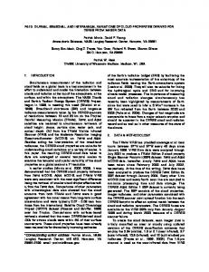
flux. The major uncertainty in CH4 fluxes exists in the biogenic flux types1 (referred to as GISS database) and since then not much has been done in a coordinated way to narrow down that range from the bottomup perspective. The anthropogenic/industrial sector emissions have been well compiled in the EDGAR database2, but with several deficiencies, e.g., annual mean emission from the rice cultivation. It is well known that the total life cycle of rice paddies span only a few months. Thus, in this study, we combine the EDGAR database with the GISS database and find the best suited CH 4 flux type combination. For this purpose, only four tracer simulations for a period of 18 years are made, and two of these are discussed here. MODEL AND DATA DESCRIPTION We have used the Center for Climate System Research/National Institute for Environmental Studies/Frontier Research Center for Global Change (CCSR/NIES/FRCGC) AGCM-based chemistrytransport model (hereafter ACTM) for simulating atmospheric CH4 at hourly time interval, horizontal resolution of T42 spectral truncation (~2.8×2.8o) and 67 sigma-pressure vertical layers has been described earlier3,4. Following chemical reactions have been considered in this simulation: CH4+O1D  Products CH4+OH  CH3 + H2O CH4+Cl  CH3 + HCl The climatological monthly-mean OH and Cl concentrations are taken from full chemistry simulations for the troposphere5 and the stratosphere6. Value of O1D is calculated online in ACTM using a climatological ozone distribution and AGCM calculated short-wave radiation at each model grid6. The trends of methyl chloroform (CH3CCl3) has been successfully reproduced using available surface emission inventory4 and model transport is validated using SF6 simulations by the ACTM3. Two emission inventories, (1) the NASA Goddard Institute for Space Studies (GISS) emission dataset1 and (2) the Emission Database for Global Atmospheric Research (EDGAR) inventory2 for biogenic and anthropogenic components, respectively, are used in combinations in ACTM (see Table 1 for details). Now for the validation of CH4 emission scenarios, we compare the forward simulation results with the observations. Firstly, with the surface measurement network, primarily based on flask sampling of ambient air at several tens of sites, operated under the cooperative program of the NOAA Earth System Research Laboratory (ESRL)7 and flux/continuous measurements at several sites by Environment Canada (EC, Canada)8, Air Sampling Network of the Federal Environmental Agency (FEA, Germany) 9, Japan Meteorological Agency (JMA, Japan)10 and National Institute of Water and Atmospheric Research (NIWA, New Zealand)11. Secondly, with the Atmospheric Infrared Sounder (AIRS) remotely sensed observations retrieved using the newly developed algorithm at the NOAA12,13. All the surface observation data are taken from the World Data Center for Greenhouse Gases (accessed 2009)14; either as the event files for the flask sites or daily/hourly average files for the continuous measurement sites. All the observational site locations are shown in Figure 1 (black symbols). However, for model-observation comparisons, we have sampled the model output along the tracks connecting the measurement sites over 6

18th International Emission Inventory Conference – “Comprehensive Inventories – Leveraging Technology and Resources”


3

longitude bands to separate the air mass characteristics originating from different continents/regions. Conventionally all the sites are joined together to evaluate the model simulated IH gradients in CH4 or other gases with more than a few years lifetime.

Table 1: Preferred CH4 emissions (Tg-CH4 yr-1) for ACTM simulation corresponding to the year 2000 (adopted from (4)). Please refer to EDGAR [http://www.mnp.nl/edgar] and GISS [http://data.giss.nasa.gov/ch4_fung/] documentations for further details on industrial and biogenic CH4 emissions used in this study. These total emissions are required to balance with modeled sinks, depending on parameters, such as the OH/Cl/O1D distributions, stratosphere-troposphere exchange (STE) rate etc. Tropospheric Budget Category

E2

E1

Industrial B-type F-type I-type L-type W-type Biogenic Termites Bio. Burn. Rice Swamps Bogs Tundra Sinks Trop. Loss Strat. Loss NH Loss SH Loss Burden

301.9 16.0 102.9 0.9 119.3 62.7 273.0 20.5 59.8 39.4 104.4 40.2 8.66 ~580 551 29 334 246 4999

261.1 13.8 89.0 0.78 103.2 54.2 312.2 --79.9 95.5 52.2 4.33

Top emission Aggr. country (E2) Emission (E2) Brazil 54.2 USA 54.0 Russia 51.3 China 47.4 India 41.1 Indonesia 30.1 Canada 17.3 Argentina 14.9 Australia 11.7 Thailand 10.7 Zaire 8.9 Nigeria 8.7 Sudan 8.6 Mexico 8.1 Venezuela 7.1 Ukraine 6.6 Vietnam 6.5 Pakistan 6.4 Peru 6.3

Top emission Aggr. country (E1) Emission (E1) India 54.2 Brazil 53.7 China 52.8 USA 44.8 Russia 42.9 Indonesia 33.2 Canada 14.4 Argentina 14.2 Thailand 13.5 Australia 10.0 Nigeria 8.7 Vietnam 8.4 Zaire 8.3 Sudan 8.1 Mexico 7.8 Pakistan 7.1 Venezuela 7.0 Ukraine 6.6 Peru 6.2



4

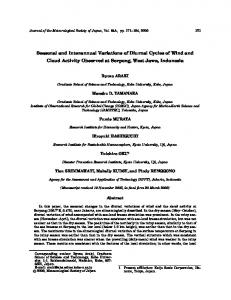
Figure 1. Surface observation network of CH4 (black circles) and model sampling locations passing over the selected sites over different continent/ocean regions are shown as the colored lines/symbols. The model sampling points are linearly interpolated between two sites at 2.5o latitude intervals along a selected transect. The sites operated by Earth System Research Laboratory, Environment Canada, Umweltbundesamt and Japan Meteorological Agency are marked in black, cyan, orange and magenta colour, respectively. RESULTS AND DISCUSSION In this work, we have compared direct and remote sensing observations with forward transport model simulations in an attempt to validate the combinations of bottom-up estimated surface fluxes for CH4. Because the ACTM transport has been validated for IH exchange time and regional scale transport using inert tracers, such as the synoptic variations in SF6 and „age‟ of air in the upper troposphere3, we believe ACTM can be utilized for this purpose. Seasonal variations of IH gradient near the earth’s surface Figure 2 shows latitudinal and seasonal variations in CH4 concentrations along 6 South-North Pole transects. Overall a good correspondence between the model and observed IH gradients are found and the



5

observed differences between different transects are clearly captured by the model simulation using E2 emission scenario. Eventhough, CH4 emissions are significantly greater during the summer months in the Northern Hemisphere (NH) than the winter months, lower atmospheric concentrations are observed over most of the regions. During the summer months, concentrations of OH, which accounts for more than 90% of CH4 loss in the atmosphere, also attain maximum values. Thus the net increase of CH4 (emission – loss) near the earth‟s surface are found during the other three non-summer months in the NH as shown in Figure 2. In the Southern Hemisphere (SH), higher CH4 concentrations are found in July/October compared to the January/April months.

Figure 2. Model-observation comparisons of seasonality in CH4 IH gradients over 6 air mass sectors (see text) as depicted in Figure 1. While observations are shown as the discrete symbols due to irregular distance between the sites, the model results using E2 emission scenario are shown as continuous lines by sampling at regular intervals in between the sites along any particular transect, covering from the South Pole station to a fictitious North Pole station. All the measurements data used in this study have been obtained from the WDCGG14.



6

One of the largest variability is found along the America transect (Figure 2b), which has alternating sites between the North America and North Atlantic. Apparently the model is able to capture the variabilities among the sites and with seasons. The KEY site show highest CH 4 level among this set of observational sites, but the modeled values peaks along this transect in the region north of LEF site. Generally, the eastern US has greater emissions (range: 0.1-5 g-CH4 m-2 mon-1) than the western US (range: 0.05-0.5 g-CH4 m-2 mon-1). The America transect also exhibits contrasting seasonality with highest modeled concentrations in July for the latitude of ~50-75oN, while all transects show lower values on an average. This contrast is mainly caused by the strong seasonality in wetland emissions (defined by Swamps, Bogs and Tundra jointly; ref. Table 1). Only at RPB, the model results are systematically underestimating the measurements by about 25 ppb in all the seasons, which can be caused due to underestimation of CH4 emission from the tropical regions of South America (eastern side) and/or northern Africa. Note also the similar or greater underestimations of CH 4 concentrations by the model at MKN. However, no such offset is seen at SEY, located in the Indian Ocean about 20 o east of MKN or tropical Pacific Ocean island sites (GMI, CHR). If compared with a recent inverse/top-down model estimated flux using SCHIAMACHY remote sensing retrievals15, we find the E2 emission scenario differs the most (less by ~7 Tg-CH4 yr-1) over the tropical South America. The fluxes in E2 scenario are 63.4, 62.9 and 50.3 Tg-CH4 yr-1, and their estimations are 70.6, 66.1 and 53.4 Tg-CH4 yr-1, respectively, for the Tropical South America, Tropical Africa and Indonesia. The CH4 concentrations at BKT site, located on the western edge of Indonesia, are well simulated for the both seasonal cycle and absolute values. Comparison AIRS CH4 in the middle to upper troposphere A balance between CH4 emission at the earth‟s surface and chemical loss in the troposphere (plus escape to the stratosphere) are required to be balanced to model the tropospheric growth rate in close agreement with the observation. Table 1 shows budget of CH4 emission and sink amounts for a reference year. This balance is also important in the UT region, in contrary to the earth‟s surface, where the CH 4 concentrations are more directly influenced by surface fluxes, i.e., before significant occurrence chemical loss and observes relatively less impact of STE. The model-observation comparison in the UT region can be considered a more complete validation of the transport modeling framework as a whole than the surface fluxes alone. Figure 3 shows the area averaged seasonal cycles of AIRS retrieved CH4 concentrations and ACTM simulations using two sets of surface fluxes (E1 and E2) in south Asia. While the seasonal cycle phases are comparable between the observation and both models, apparently an average of the two model simulations fits the AIRS retrievals the best. This comparison leads to a suggestion that the total CH4 emission is underestimated (overestimated) in the E2 scenario during the summer (winter) season, and, on the contrary, the total emission is overestimated for the E1 emission scenario in the summer. Both are able to capture the annual mean concentrations fairly well (within 30 ppb). Figure 4 (bottom row) shows a significant increase of CH4 in August in the middle to upper troposphere in Southeast Asia, and this enhancement is associated with both rapid vertical transport due to the active phase of the Indian summer monsoon3 and highest surface emission intensity due to rice paddies as used in ACTM (source: (1)). Some difference of the location and amplitude of the enhancement over the Asian continent is evident between model simulation and satellite observation in



7

August. The overestimation in E1 scenario is consistent with the comparison of satellite observation with model TM3 over South Asia13. In addition, there are also some differences in horizontal distribution patterns, with two elevated CH4 regions over India and China in AIRS observations in comparison to one in ACTM simulation. During February (Figure 4; top panel), the ACTM simulated concentrations are higher by about 20 ppb compared to that retrieved by AIRS. The model shows transport of CH 4 rich air from the Europe/Siberia to north-east China by the prevalent westerly winds (ref. Figure 5c).

Figure 3. Seasonal cycles averaged over the Asian monsoon domains (left: 65-80oE; right: 80-110oE) as retrieved from the AIRS and simulated by ACTM using two emission scenarios. The annual mean value has been subtracted from each curve separately. On reversal of CH4 seasonal cycle at mid-troposphere (at ~300 mb) Surface measurements and model simulations at the surface layer exhibit a summer minima and winter maxima at all latitude bands. On the other hand, as seen from Figure 4 (left column), the AIRS observations at 350-250 mb height exhibit opposite seasonality. We find, a reversal of seasonality in northern mid- to high latitudes (higher values in summer compared to the winter) with respect to that has been observed near the surface (ref. Fig. 2 and associated discussions). Study of the monthly-mean horizontal distributions of CH4 at three layers (400, 300, and 200 mb) for February and August suggest that this seasonal cycle phase reversal occurs at about 300 mb. The 200 mb layer is mostly located in the stratosphere during the NH winter as mixing ratio of SF6 decreases poleward in the range of 30-90oN (not shown), which is not observed south of 60oN at 300 mb level because SF6 has no photo-chemical loss in the troposphere and stratosphere. A strong decrease in SF6 mixing ratio with altitude, compared to the IH gradient, is well known as result of slow transport of air vertically upward in the stratosphere 3. The lower CH4 concentration located north of 60 oN about 120oW are coincident with lower SF6 concentrations over



8

this region. Thus the reversal of CH4 seasonality at ~300 mb is caused mainly by the intense stratospheretroposphere exchange within the polar vortex. The 300 mb layer may be located in the stratosphere sometimes16. These aspects will be analyzed further in the future.

Figure 4. Latitude-longitude distribution of CH4 mixing ratio as retrieved from the AIRS instrument (left column) in comparison with ACTM model simulations using E2 (middle column) and E1 (right column) for the months of February (top) and August (bottom).

The vertical transport of elevated CH4 air (also seen in Figure 4) by the Indian summer monsoon in August can be seen clearly in Figure 5 (right column). Interestingly, highest CH 4 concentrations are found at 200 mb level over the Tibetan plateau region, compared to the 300 or 400 mb levels. This special feature in CH4 arising from monsoon dynamics can be easily visualized using the „age‟ distribution of the tropospheric air (see (3) for detailed discussion). They found the air around 200 mb to be the youngest over the deep cumulus convection zones in the tropics (SH summer in February, NH summer in August), compared to any other heights above about 500 mb. It should also be pointed out here the mean circulation forced by the high orography in the Himalayan region also plays a role in uplifting the surface emission to the upper troposphere.



9

Figure 5. Latitude-longitude distributions of CH4 as modeled using ACTM are shown for three layers in the mid- and upper troposphere. The wind vectors are also shown to indicate transport pathways of high and low CH4 air at these altitudes.



10

CONCLUSIONS AND OUTLOOK Using the model-observation comparison we have found an optimal combination of various flux types to be used in forward transport modeling of CH 4. Although the global total flux appear to be dependent on the chemistry-transport model parameters, such as the radicals and STE rates, which can be adjusted by changing total anthropogenic emission, a rather tight constraint is achieved for the biogenic flux components. We have illustrated that with the present day observation network of atmospheric CH 4 near the earth‟s surface, more information on surface fluxes can be extracted by selecting different longitudinal sectors for the latitudinal profiles (IH gradients) and separating them seasonally. Since the latitudinal profiles looks distinct over different land and oceanic regions, applying the inverse modeling tools the CH4 fluxes can be constrained for the longitude bands covering the ocean or the land regions. Horizontal distributions with continuous coverage are obtained from the AIRS on board the Aqua satellite and comparisons with ACTM simulations suggest that strong surface emission coupled with efficient vertical transport by the deep cumulus convection create large enhancement of CH 4 at the 350250 mb height. Such situation is well supported by an analysis of age of air in the tropical troposphere. However, some disagreements exist between the AIRS-ACTM comparison during the NH winter and around the high latitude regions. Further improvements in the model simulations as well as the remote sensing retrieval are needed to eliminate and understand the causes of these discrepancies. A reversal of seasonal cycle is seen at about 300 mb, from summer minimum and winter maximum below 300 mb to summer maximum and winter minimum at 300 mb and above. This is diagnosed to be caused mainly by the STE in the polar vortex region during the NH winter, with the help of similar plots of SF6 distributions. ACKNOWLEDGEMENTS. We thank NIWA for providing BHD and ARH data freely. We appreciate support of Takakiyo Nakazawa and Hajime Akimoto for conducting this research at FRCGC. REFERENCES 1. Fung, I., J. John, J. Lerner, E. Matthews, M. Prather, L. P. Steele, and P. J. Fraser “Three-dimensional model synthesis of the global methane cycle”, J. Geophys. Res. 1991, 96, 13033–13065. 2. Olivier, J. G. J., and J. J. M. Berdowski “Global emissions sources and sinks”, The Climate System; J. Berdowski, R. Guicherit, and B. J. Heij (eds.), A.A. Balkema Publishers/Swets & Zeitlinger Publishers; The Netherlands, ISBN 9058092550, 2001, pp 33-78. 3. Patra, P. K., M. Takigawa, G. S. Dutton, K. Uhse, K. Ishijima, B. R. Lintner, K. Miyazaki, and J.W. Elkins “Transport mechanisms for synoptic, seasonal and interannual SF6 variations and “age” of air in the troposphere”, Atmos. Chem. Phys. 2009a, 9, 1209-1225. 4. Patra, P. K., M. Takigawa, K. Ishijima, B.-C. Choi, D. Cunnold, E. J. Dlugokencky, P. Fraser, A. J. Gomez-Pelaez, T.-Y. Goo, J.-S. Kim, P. Krummel, R. Langenfelds, F. Meinhardt, H. Mukai, S. O'Doherty, R. G. Prinn, P. Simmonds, P. Steele, Y. Tohjima, K. Tsuboi, K. Uhse, R. Weiss, D.



11

Worthy, T. Nakazawa “Growth rate, seasonal, synoptic and diurnal variations in lower atmospheric methane”, J. Meteorol. Soc. Jpn. 2009b, in review. 5. Sudo, K., M. Takahashi, J. Kurokawa, and H. Akimoto “CHASER: A global chemical model of the troposphere 1. Model description”, J. Geophys. Res. 2002, 107, 4339. 6. Takigawa, M., M. Takahashi, and H. Akiyoshi “Simulation of ozone and other chemical species using a Center for Climate System Research/National Institute for Environmental Studies atmospheric GCM with coupled stratospheric chemistry”, J. Geophys. Res. 1999, 104, 14003– 14018. 7. Dlugokencky, E.J., L.P. Steele, P.M. Lang, and K.A. Masarie “The growth rate and distribution of atmospheric methane”, J. Geophys. Res. 1994, 99, 17021-17043. 8. Worthy, D. E. J., I. Levin, N. B. A. Trivett, A. J. Kuhlmann, J. F. Hopper, and M. K. Ernst “Seven years of continuous methane observations at a remote boreal site in Ontario, Canada”, J. Geophys. Res. 1998, 103, 15995–16007. 9. Uhse, K., F. Meinhardt, and L. Ries “Atmospheric CH4 hourly concentration data, Schauinsland, Zugspitze/Schneefernerhaus”, Air Monitoring Network of the Federal Environment Agency (available at WDCGG, http://gaw.kishou.go.jp/wdcgg.html) 2009. 10. Tsutsumi, Y., K. Mori, M. Ikegami, T. Tashiro, and K. Tsuboi “Long-term trends of greenhouse gases in regional and background events observed during 1998-2004 at Yonagunijima located to the east of the Asian continent”, Atmos. Environ. 2006, 40, 5868-5879. 11. Lowe, D. C., C. A. M. Brenninkmeijer, G. W. Brailsford, K. R. Lassey, A. J. Gomez, and E. G. Nisbet “Concentration and 13C records of atmospheric methane in New Zealand and Antarctica: Evidence for changes in methane sources”, J. Geophys. Res. 1994, 99, 16913–16925. 12. Xiong, X., C. Barnet, E. Maddy, C. Sweeney, X. Liu, L. Zhou, and M. Goldberg “Characterization and validation of methane products from the Atmospheric Infrared Sounder (AIRS)”, J. Geophys. Res. 2008, 113, G00A01. 13. Xiong, X., S. Houweling, J. Wei, E. Maddy, F. Sun, C. D. Barnet “Methane Plume over South Asia during the Monsoon Season: Satellite Observation and Model Simulation”, Atmos. Chem. Phys. 2009, 9, 783-794. 14. WDCGG “WMO World Data Centre for Greenhouse Gases”, Japan Meteorological Agency, Tokyo (data available at http://gaw.kishou.go.jp/wdcgg.html), Tokyo 2009. 15. Frankenberg C., P. Bergamaschi, A. Butz, S. Houweling, J. F. Meirink, J. Notholt, A. K. Petersen, H. Schrijver, T. Warneke, I. Aben “Tropical methane emissions: A revised view from SCIAMACHY onboard ENVISAT”, Geophys. Res. Lett. 2008, 35, L15811. 16. Sudo, K. 2009. Frontier Research Center for Global Change, Yokohama, personal communication.
