Handling Heterogeneity in Networked Virtual Environments 1
Helmuth Trefftz 1, Ivan Marsic 2 and Michael Zyda 3 and CAIP Center, Rutgers University 3 The MOVES Institute, Naval Postgraduate School
[email protected],
[email protected],
[email protected] 2
Abstract The availability of inexpensive and powerful graphics cards as well as fast Internet connections make Networked Virtual Environments viable for millions of users and many new applications. It is therefore necessary to cope with the growing heterogeneity that arises from differences in computing power, network speed and users’ preferences. This paper describes an architecture that accommodates the heterogeneity mentioned above while allowing a manager to define system-wide policies. Policies and users’ preferences can be expressed as simple linear equations forming a mathematical model that describes the system as a whole as well as its individual components. When solutions to this model are mapped back to the problem domain, viable solutions that accommodate heterogeneity and system policies are obtained. The results of our experiments with a proof-of-concept system are described.
1. Introduction Powerful computer graphics cards are becoming less expensive and most new computers ship with cards that are capable of displaying complex 3D scenes at interactive rates. Similarly, high-speed connections to the Internet are becoming increasingly common. These facts allow for a potential widespread use of Distributed Virtual Environments (DVEs) or Networked Virtual Environments, as described in [6]. In a controlled environment, the DVE designer can determine a-priori the type of computers and network connections that will be involved in the system. The DVE can then be engineered to perform well within the given conditions. But as DVEs find their ways to real world applications, the environments cannot be so easily controlled. Heterogeneity arises in different forms: • Nodes with a wide variety of computing resources (processor speeds, available memories, graphic cards). • Varying connection type of the nodes (from modem lines to local area networks). On the other hand, designers of DVEs need to be able to determine certain system-wide constraints in order to guarantee productive use of the system. Examples of
these policies are: maximum number of concurrent users, minimum frame-rate that each node must be able to maintain, maximum number of messages per unit of time that can be handled by the system, etc. On one hand then, we have the heterogeneity that arises from the diverse participating nodes and from individual users preferences. On the other hand we have the need to provide the designer with the ability to dictate and enforce certain homogeneity of function.
1.1. Contributions of this Work In this paper, we propose a client-server architecture that we call Switchboard Architecture (SA) that copes with the conflicts described above. The structure of the SA makes it possible to map individual user preferences as well as system constraints to linear equations and inequalities. This set of equations and inequalities form a mathematical model that describes how the system functions. Valid solutions to the mathematical models are isomorphic with states of the DVE in which individual users’ preferences are satisfied as closely as possible given the restrictions imposed by the hardware and the constraints defined by the DVE designer. There are two main contributions of this work: • The Switchboard Architecture, which can be used in other client-server DVEs. • The mathematical model that approximates the functioning of the DVE system. The model provides an objective and automatic way to cope with the opposing tendencies of heterogeneity and homogeneity in DVEs. The rest of this paper is organized as follows: Section 2 describes related work. Section 3 describes the Switchboard Architecture, as well as the generic form of the corresponding mathematical model. Section 4 and 5 describe the results we have obtained with a shared visualization program we have built incorporating the principles we describe. Section 6 presents the conclusions and future work.
2. Related Work One of the most desirable conditions in a DVE is to provide all participants with a consistent and up-to-date
version of the shared space. But in the presence of imperfect communication channels, the time to replicate the shared state among participants is not zero, giving rise to the Consistency-Throughput tradeoff [6]. As the number of participants and entities taking part in the DVE increase, the number of messages and the amount of computation necessary to keep a consistent version increase exponentially. An important related area of research in DVEs deals with the architecture for building a DVE system. An extensive survey of architectures can be found in [4] . A large amount of research in DVEs has been dedicated to reducing the number of messages and the computational load needed to keep a consistent, yet possibly distributed, description of the virtual world, with the main objective being scalability. One area of research that addresses this problem deals with Area of Interest Managers (AOIM). Only messages pertaining to the current area of interest of the users are conveyed to their nodes with high priority. Macedonia [5] describes a way to map multicast groups to geographical regions. As a user traverses the simulation field, he/she leaves some regions and enters others, changing the multicast groups he/she uses to exchange message with other participants in the same regions. Having several levels of representation for the virtual objects can also reduce the amount of computation done at each node. Objects that are far from the observer or of less interest for the user can be rendered with lower fidelity. Capps [1] defines a framework for managing the display and request of representations for virtual objects called QUICK. Objects are annotated with a measurement for Quality, Importance and Cost. The system optimizes the total fidelity contribution while minimizing the cost. Reducing the number of messages used to keep a consistent state of the system is another goal. Most of these techniques make use of dead reckoning, which involve sending not only the position but also the trajectory of a moving object. If each participant can locally compute the position based on the trajectory, only changes to the trajectory need to be sent. Faisstnauer et al. [2] propose an algorithm to schedule outgoing messages. Messages that describe updates to objects that deviate more from their previously sent trajectories are given higher priority. The result is that the overall system-wide error is minimized. In small DVEs, the differences in performance between the participating nodes can also be exploited. If a particular node is sending updates faster than the other nodes can process them, bandwidth and resources are being wasted. In a previous paper [9], we explored this issue and obtained a decrease in bandwidth utilization as well as improved responsiveness in slower nodes. Terrence and Dew [8] make a theoretical characterization on the number of
messages that can be dropped in order to keep a good frame rate in a Collaborative Environment. Being able to manage the Quality of Service provided to the participants is a desirable feature. Greenhalgh et al. [3] propose a system that allows users to exchange video streams in a virtual environment. The scarce multicast groups are assigned to users based on the interest of the users and their proximity in the virtual environment.
3. Our Approach As discussed in the introduction, conflict can arise between the constraints imposed by the designer of a CVE and the heterogeneity that results from node diversity and user preferences. Our approach provides a mapping from the system-design domain to a mathematical domain. This mapping is accomplished by modeling the user preferences and the administrator constraints as equations. Since a mathematical correspondence can be defined between these two domains, solving the model in the mathematical domain provides for an objective and fair solution in the systemdesign domain. These relationships are depicted in Figure 1. We discuss below how the mapping between the two above-mentioned domains can be accomplished.
3.1. Mathematical Model The different dimensions of shared information that can be tuned by the user and, possibly, be enforced by global policies in the system, are called variables. Examples would include: the number of video frames per second; the quality of visualization (wire-frame, shaded, etc.); the quality of sound (mono, stereo, 3D, etc.). Variables take on discrete possible values within a certain range, determined by the computing power of the nodes taking part in a session. The Cartesian product of the possible values of the different variables forms an ndimensional search space, n being the number of variables. Assigning a fixed value to a variable can Policies/Preferences
Solution
Mathematical Model
Mathematical Solution
Figure 1. Mappings between the design and math domains.
directly affect the amount of computing power dedicated to processing data related to it. Variables that are fixed in this manner are called independent variables. The designer might allow the operating system to freely allocate computing power to other variables, which will then take values depending on the fixed-value variables and other factors. These are called dependent variables. Our approach works by controlling certain variables and letting the operating system (OS) assign all remaining computing power to the dependent variables. The amount of computing power dedicated to the dependent variables will depend on the total computing power of the node, the availability of specialized processors and OS scheduling policies. The value of the dependent variables will therefore vary from one node to another. The values that the dependent variables take in a particular node, for a given set of independent variables, depend on the performance of each node. This mapping is called the performance mapping. The performance mapping is determined by a set of benchmarks run at each participating node before the beginning of the collaborative session. Global policies can be expressed as inequalities over certain variables. An example of a global policy might be: “Each system must be able to display at least 2 video images per second”. An Individual’s preferences can be expressed as a linear combination of the variables. The normalized coefficients of the variables determine their relative importance. Normalization of the coefficients must be done carefully, taking into account the ranges of the involved variables. Global policies partition the space into valid subspaces. The intersection of these valid subspaces is, in turn, either a finite or an infinite n-dimensional space. In order to enforce the global policies, variables at each node are limited to taking only values that lie inside the intersection of valid subspaces. The points of the search space that lie inside the intersection of valid subspaces form the valid search space. The linear combination of variables that describes the individual preferences becomes the objective function, which needs to be maximized. The function is evaluated at each point of the valid search space looking for a maximum. The optimum values of the dependent variables are assumed to be the results of the performance mapping at the point that maximizes the objective function. The user controls the coefficients of the objective function through a control panel with one sliding control for each variable. Moving up the slider for one variable means assigning more relative importance to it, at the expense of another variable(s). The mathematical model consists of the following parts: • Each user’s objective function, of the following form:
Max ∑ Wi × I i + ∑ W j × D j j i
(1)
Here, I are the normalized values of the independent variables; D are the normalized values of the dependent variables; W are the weights representing the user’s preferences. • Constraints representing minimum information representation levels have the following form:
Ii ≥ Ki
(2)
K is the minimum level of information representation allowed for variable Ii. • Constraints limiting the maximum number of messages the server can process per unit time have the following form:
∑V
k
≤ Li
(3)
k
Here, L is the maximum number of messages related to variable V that the server can process per unit time. Sub-index k covers all participants in the CVE. Linear equations of type (1), (2) and (3) together form the mathematical model, which is similar in form to a linear programming problem. But the model cannot be handled with linear programming techniques because the variables do not take continuous values and because the dependent variables are not linear with respect to the independent variables (recall that the values of the dependent variables are obtained experimentally via the performance mapping). However, given the small size of the search space, the objective function can be evaluated at each valid point in order to find the maximum very quickly. The values of the variables at the point where the objective function is maximized correspond to the fidelity level that the client must set in order to adapt as well as possible to the user’s preferences while complying with the global policies. Our approach works in two phases. • Off-line: Prior to actively joining the session, each node runs a series of tests. During the tests, the node is set to work under the Cartesian product of the independent variables, and the values of the dependent variables are measured and recorded (performance mapping). Thus, the search space is predetermined for each node. It is assumed that
•
every node’s behavior will remain relatively constant. On-line: During the collaborative session, the system needs to adapt to changes that may occur. For instance, the user might change her preferences, thereby changing the relative importance of the variables. A new search for the maximum value inside the local valid search space has to be conducted. Or a new user might join the session, adding to the number of messages the server has to process.
3.2. The Switchboard Architecture The architecture we propose is described in Figure 2. The server receives updates from the clients and distributes those updates into the switchboard matrix according to each client’s capacity and user preferences. Each row of the switchboard handles a variable in the system. Updates for a specific variable from all the participating clients are received in the “receiving-plug” (Figure 2). The message is then buffered in a small cache at each “transmitting-plug”. Each transmitting plug has an associated timer controlling its transmission period. When the timer expires, all the updates stored in the plug’s cache are transmitted to the subscribed clients (if
Server
Variable 1
…
Variable 2
… …
…
…
… Variable m
…
Client 1
Client n
Figure 2. The Switchboard architecture.
Each “plug” corresponds to a specific combination of variable and information fidelity. The column vector on the left represents the receiving plugs and the matrix on the right represents the transmitting plugs.
any). In order to reduce traffic, each “transmitting-plug” is implemented as a multicast group. In Figure 2, two clients and the server are described. Receiving-plugs are represented as the column on the left inside the Server rectangle. Transmitting-plugs are represented as the matrix on right hand side of the rectangle. Transmitting-plugs corresponding to more frequent updates are located at the right hand side of the matrix. Note that updates coming from both clients arrive
at the same receiving-plugs (one per variable). Client n, running on a fast computer, subscribes to the highest frequency of updates for variables 1 and 2, and to the lowest frequency of updates for variable m. The user on client n is more interested on variables 1 and 2 than on variable m. Client 1, running on a slow machine, subscribes to the slowest frequency of updates for variables 1 and m, and to a rather slow frequency for variable 2. The user at client 1 is more interested in variable 2 than on variables 1 and m. The effect of this architecture is that the server acts as a buffer, providing slower nodes with a sub-sample of messages generated by faster nodes in a controlled manner that is determined by the client node’s capacity and users’ preferences. The apparent jumpiness of the objects which are updated less frequently can be compensated, to an extent, with dead-reckoning.
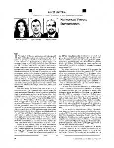
4. Experimental Setup As a proof of concept for the architecture and the model, a shared visualization system was built using Java3D [7] . Figure 3 shows a screenshot of the system. Three users meet virtually to discuss over a shared visualization data set. Users utilize “telepointers” (3D arrows) as means to point inside the virtual world. Small video windows are provided to allow users to see the faces of the other participants. Only one user can manipulate the visualized object at a given time. The application directly handles all the media related to the variables in order to be able to optimize the objective function. We could use third party applications, e.g., for video conferencing, if they provide APIs to control the level of fidelity and the statistics on the number of lost messages.
4.1. Variables • • • • •
The variables involved in the system are: T: Telepointers update rate. O: Visualization dataset update rate. V: Video update rate G: Graphical representation fidelity F: Scene visualization frame rate.
Variables T, O, and V can take the following values: 0 (no updates), 1, 2, 10 or 20 updates per second. Variable G can take value 0 (wire-frame representation) or 1 (Phong shaded). Another use of variable G could be different levels of detail of the visualization dataset. Higher level of detail would correspond to larger values of G.
Variables T, O, V and G are independent variables. Variable F is the dependent variable. The values F can take are the result of the performance mapping, and vary considerably across machines. Before using the values of the variables in the objective function, they must be normalized by dividing the current value by the maximum value of that variable. This operation maps the values of the different variables into dimensionless numbers between 0 and 1. Each number expresses what fraction of the maximum fidelity level is set by the current variable value. Note that the maximum value for F is node-specific and is found during the performance mapping. The ranges of the variables can be defined with finer granularity, thereby increasing the controllability of the system. But the search space would become larger and the search more expensive. The sliders shown in Figure 3 provide users with a way to assign relative weight to the variables. The values of the sliders are normalized in order to obtain the coefficients for the objective function as follows:
Wi =
Si ∑ Si
(4)
i
Si are the values of the sliders, between 0 and 100. Wi are the values of the coefficients used in the objective function, Eq. (1). Note that the selection of the variables for the model is
Figure 3. Screenshot of the system. Telepointers are represented as 3D arrows. The sliders allow the user to set the relative weights of different variables.
specific to the application. In a battlefield simulation, for instance, one variable might be assigned to slow moving vehicles, such as tanks and another to fast moving vehicles, such as airplanes. Users of one type of vehicle will probably be more interested in (and will assign higher priority to) messages originating from vehicles of similar type.
4.2. Scenario for Applying the Model Here we describe a typical scenario for employing our mathematical model in a collaborative session. Initially, a benchmark program is run on each node in order to create the data for its particular performance mapping. The node subscribes sequentially to every point in the Cartesian product of the dependant variables for a certain period long enough that the behavior of the dependent variables stabilizes. In our case the dependent variable is frame rate and the required time is 5 seconds. The dimension of the search space in our example is 250 (5 × 5 × 5 × 2). During that time, the server generates fake updates for telepointers, object movement and video. Each message is marked with a sequence number, in order to detect lost messages. At the node, an entry is added to a vector every time a frame is displayed in order to determine the average frame rate for the particular search space vertex. Additionally, for each message that is processed, an entry is added to a vector, in order to determine the number of lost messages at each search space vertex. When the benchmark finishes, the vectors are saved to disk and summarized in a particular performance mapping for the node. Next, the collaborative session starts. Initially, the optimizer module in the client finds the solution that maximizes the objective function that corresponds to all the sliders at 50 (the sliders can take values between 1 and 100). The client then subscribes to the server to the appropriate “plugs” and sets the fidelity of the visualization dataset according to the current solution. Information exchanged between the client and the server regarding the mathematical model is meta-data and is sent through a TCP connection. When the user moves the sliders in order to adjust the relative importance of a variable, the optimizer module finds a new solution. The search involves evaluating the polynomial that represents the objective function at the valid vertices (250 or less, since some of the search vertices are marked as invalid). As result, it might be necessary to unsubscribe from a particular plug (associated with a fidelity level of a variable) and subscribe to a different one. Finally, the flow of the actual data between the client and the server proceeds as described in Section 3.2. In the example system, each plug is associated with a non-
Bochica: frame rate vs (video x telep)
Bachue: fram e rate vs (video x telep) 40 35 30 25 20 15 10 5 0
14 12 10 8 6 4 2
10
0
telep
0
1
2
10
video
20
0
0
1
2
10
20
telep
0
video
Figure 4. Bochica: Impact of video and telepointer updates on the frame rate. reliable multicast group and information is transmitted via UDP. In our current implementation, if a node is subscribed to receive a particular frequency of updates for a specific variable, it will also send updates for that variable at the same frequency. This is necessary in order to enforce equations of type (3), and allows the designer to specify upper limits on the number of messages the server will need to process for each variable.
5. Results
Figure 5. Bachue: Impact of video and telepointer updates on the frame rate. human digestive system, and consists of 27,202 vertices.
Table 1. Computers used in the experiments Processor
Morlak: Video Drop vs. video x telep
1 0.8 0.6 0.4 0.2 10
0 0 20
10
2
1
0 telep
Figure 6. Percentage of video messages dropped depending on the number of video and telepointers messages per second (in Morlak).
Bochi ca Morla k
Processo r Speed
Graphics Card Memor y 1 GB
Pentium 4
1400 MHz
dual Pent III
730 MHz
1 GB
FireGL 1 – 32MB
Pentium II
500 MHz
256 MB
Intense3D – 16 MB
Bachu e
Table 1 gives the characteristics of the computers used for the experiments. The visualization dataset we used for these particular experiments is a representation of the
video
10
GeForce2 – 32MB
The complete performance mapping cannot be graphed because it involves five (5) different variables. But a plot of the visualization frame rate (F) versus telepointers update (T) and video frame rate (V) is shown for Bachue and Bochica in Figures 4 and 5. Note the difference in the scale. Note also that as the frequency of video messages increases, the frame rate decreases noticeably, whereas the impact of more frequent telepointer messages is small. Video messages have a larger impact on the simulation than telepointers messages. The solutions suggested by the math model are sensible and consistent with the data captured in the performance mapping. For instance, when the maximum priority is assigned to frame rate, the system lowers the resolution of the model to wire-frame and reduces the
frequency of the video updates, which negatively impact the frame rate, as shown in Figures 4 and 5. The number of lost messages is an important parameter for measuring degradation of the system. Slower nodes drop more messages than faster ones under the same load. Again, as the number of messages for a specific variable increase past a certain threshold, so does the number of lost messages. Figures 6 and 7 show how the number of lost video messages grows for Bochica and for Morlak. Note that Bochica is capable of handling video messages without dropping any until the frequency exceeds 10 messages per second. In Morlak, a percentage of messages is always dropped. Notice also the difference in scale. Bochica does not drop more than 6% of video messages, whereas Morlak drops up to 95% in the worst-case scenario. We have incorporated the number of dropped messages during the benchmarks to the algorithm that finds the solution. Particular points in the Cartesian product of variables that are found to cause too many dropped messages cannot be chosen as solutions. If the number of dropped messages is not considered, these points appear as good candidates for the solution, because the frame rate increases as messages are dropped and need not be processed. In our current experiments, we mark a point non-valid if it causes more than 50% drop in messages of any variable. In a real life application, different thresholds could be applied to different variables, according to the user’s perception and/or relative importance. Since the mathematical model is based on actual data collected through the benchmarks, the solutions found for the same set of slider values (directly related to the objective function coefficients) vary considerably across nodes. Table 2 shows the solutions found at the different nodes for the same set of user’s slider values. The user’s sliders were set to . This set of sliders values assigns the highest importance to frame rate, some importance to the graphical representation of the model and very little to the remote events. Note that in both Bochica and Bachue (the faster machines) updates from the telepointers and objects can still be received at maximum speed, without affecting the frame rate. Morlak, on the other hand, has to reduce the frequency of all remote updates. Note also that all nodes, fast and slow, need to reduce the frequency of video updates, which have a big impact on the frame rate. Table 2. Solutions found at the different nodes for the same set of user sliders values. Teleptr.
Object
Video Resol’n .
Bochica: Video Drop vs. video x telep 0.06 0.05 0.04 0.03 0.02 0.01
10 video
0 0
2 20 10
1 0 telep
Figure 7. Percentage of video messages dropped depending on the number of video and telepointers messages per second (in Bochica).
Morlak Bochic a Bachue
1 20
2 20
1 2
1 1
20
20
1
1
In order to test the improvement in frame rate when utilizing the proposed architecture, a node was set to simulate 20 updates per second for each variable (telepointers, object, video). Data was collected about the frame rate at each node with and without the Switchboard Architecture. The results are shown in Figure 8. The largest improvement is naturally obtained for the slowest machine, which benefits most from the buffering effect of the server. The frame rate increases found were as follows: Bachue: 33%, Bochica 10% and Morlak 366%.
6. Conclusions and Future Work We have presented the Switchboard Architecture and the underlying mathematical model. Current results show that the architecture provides an effective way of enforcing global constraints while allowing users to modify the characteristics of the user interface according to their preferences. The situations that can benefit from the framework we propose can be characterized as follows: • Participating nodes have diverse degrees of computing power. • The modalities for sharing information can be represented with varying degrees of fidelity in space/time dimensions.
•
There is not enough computing power at each and every node to represent at the same time all the modalities at their maximum level of fidelity. Fram e Rate Increase (%)
the statistics collected during the benchmark have to be extrapolated based on the current statistics collected during the collaborative session. We are currently experimenting with different formulations for this extrapolation.
Acknowledgements
4 3 2
N o S .A . S .A .
1 S .A .
0
N o S .A . B achue
B ochica
The work presented in this paper was sponsored by Eafit University, NSF Contract No. ANI-01-23910 and the Rutgers CAIP Center. The authors are grateful to Professor Manish Parashar, from Rutgers University, for his ideas and comments on how to make the model adaptive.
M orlak
References Figure 8. Increase in Frame Rate in the presence of the Switchboard Architecture and the solutions described in table 2.
In such an environment, our solution allows the following to happen in a controlled manner: • Users can choose the fidelity or the modality for information presentation to meet their preferences (within globally specified restrictions or policies). • A global administrator can define global policies regarding minimum requirements for information representation/sharing, as well as the maximum number of messages the server can process per unit of time. The data collected in the benchmarks that are run before the collaborative sessions form a static snapshot of the system. If conditions change during the collaborative session (for instance if the network becomes congested), the current system does not have a way to react to the change. We thus plan to explore how to add dynamic monitoring and adaptation under changing conditions. In order to make the system adaptive, it is necessary to collect, during the collaborative session, the same statistics that are collected during the benchmarks, that is: frame rate and percentage of dropped messages. If the percentage of dropped messages exceeds the upper bound, the current solution is temporarily marked as invalid. In this case, the optimizer module has to be invoked in order to look for a new solution. Since the optimizer module uses the whole search space as input,
[1] Capps, M.V. Fidelity Optimization in Distributed Virtual Environments. Ph.D. thesis, Naval Postgraduate School, Monterey, CA 2000. [2] Faisstnauer, C., D. Schmalstieg and W. Purgathofer. “Priority Round-Robin Scheduling for Very Large Virtual Environments”. Proceedings of IEEE VR 2000, pp. 135 – 142. [3] Greenhalgh, C., S. Benford and G. Reynard. “A QoS Architecture for Collaborative Virtual Environments”. In Proceedings of ACM Multimedia 1999, pp. 121 – 130. [4] Macedonia M.R. and M. Zyda. “Taxonomy for Networked Virtual Environments”, IEEE Multimedia, 1997, pp. 48-56. [5] Macedonia M.R. A Network Software Architecture for Large-Scale Virtual Environments. Ph.D. thesis, Naval Postgraduate School, Monterey, CA 1995. [6] Singhal, S. and M. Zyda, Networked Virtual Environments, ACM Press, New York, 1999. [7] Sowizral, H., K. Rushforth and M. Deering. The Java 3D API Specification. Java Series. Addison-Wesley, December 1997. [8] Terrence F. and P. Dew. “A Distributed Virtual Environment for Collaborative Engineering”. In Presence, Vol 7, No 3, June 1998, pp 241 – 161. [9] Trefftz H. and I. Marsic. “Message Caching for Global and Local Resource Optimization in Shared Virtual Environments”. Proceedings of VRST 2000, pp. 97 – 102.