2 The Courant Institute of Mathematical Sciences and Center for Neural Science, New York University, USA. Abstractâ We present a hardware-accelerated ...
Hardware Accelerated Visual Attention Algorithm Polina Akselrod1, Faye Zhao1, Ifigeneia Derekli1 , Cl´ement Farabet1,2, Berin Martini1 Yann LeCun2 and Eugenio Culurciello1 1
2
Electrical Engineering Department, Yale University, New Haven, USA The Courant Institute of Mathematical Sciences and Center for Neural Science, New York University, USA
Abstract— We present a hardware-accelerated implementation of a bottom-up visual attention algorithm. This algorithm generates a multi-scale saliency map from differences in image intensity, color, presence of edges and presence of motion. The visual attention algorithm is computed on a custom-designed FPGA-based dataflow computer for general-purpose state-of-theart vision algorithms. The vision algorithm is accelerated by our hardware platform and reports ×4 speedup when compared to a standard laptop with a 2.26 GHz Intel Dual Core processor and for image sizes of 480 × 480 pixels. We developed a real time demo application capable of > 12 frames per second with the same size images. We also compared the results of the hardware implementation of the algorithm to the eye fixation points of different subjects on six video sequences. We find that our implementation achieves precisions of fixation predictions of up to 1/14th of the size of time video frames.
I. I NTRODUCTION Visual attention algorithm have been a subject of intense research for many years. Several models of visual attention have been proposed to identify image location of interest and saliency, and to model the way human observers move their eyes in response to bottom-up features in the image [1], [2], [3], [4], [5]. Visual attention is used not only to predict the visual attractiveness of locations in an image, but also to guide vision towards target objects of interest. It is also used in psychophysics experiments with complex stimuli in an effort to understand the human visual system However, computing attention algorithms is computationally intense. This issue becomes critical in real-time applications dealing with largescale images. In this paper, we describe a hardware-accelerated implementation of a visual attention algorithm, based on the model described in ”A model of saliency-based visual attention for rapid scene analysis” by L. Itti, Ch. Koch & E. Niebur [1]. The core computations of the algorithm are performed on our custom-designed hardware named NeuFlow [6]. This system was developed with the purpose of accelerating generalpurpose vision algorithms [7], [8]. The use of hardware allowed us to run the algorithm in a real-time application at over 12 frames per second for images of size 480 × 480. This paper has the following organizartion: in Section II, we describe the visual attention model on which we base our implementation. In Section III, we briefly discuss the NeuFlow hardware system, that we used to accelerate the algorithm. In Section IV, we describe the implementation details as well as several modifications of the original model that we have introduced. In Section V, we report on several experiments that
aim at validating the performance and evaluating the running time. Section VI concludes the paper. II. A LGORITHM The vision algorithm we used in this paper is based on the model, described in [1]. The goal of the algorithm is to locate the points of visual attention in the input RGB image (or video). For this purpose, several feature maps are computed. These maps indicate differences in intensity and color, and report edges and motion in the scene. The linear combination of the feature maps yields the saliency map. To detect fine as well as coarse details of the input image, a pyramid of scales is used. Different scales are obtained by subsampling the maps. The final saliency map is a linear combination of interpolations of intermediate saliency maps on different scales. The maxima of the saliency map are defined to be the principal points of visual attention. Due to our custom hardware, we have introduced a few modifications (see Section IV for more details). Below we describe the algorithm that we used to calculate all the feature maps and the saliency map. Suppose that A is the input image with 3 color channels, denoted by R, G, B. The intensity feature map I is defined by equation 1. I = 0.299 · R + 0.587 · G + 0.114 · B
(1)
In other words, intensity is a weighted average of the three channels. To detect the difference in color, we define two feature maps RG (red-green) and BY (blue-yellow) by equation 2, 3. RG =
R−G I
(2)
B − (R + G)/2 (3) I The edges feature map E is computed by convolving the intensity map I with the 3 × 3 Laplacian kernel (Ker) , as in equation 4. BY =
0 −1 0 E = I ∗ Ker; withKer = −1 4 −1 0 −1 0
(4)
The motion is detected by calculating the temporal difference T D between the intensities of two consecutive frames I1
and I2 of the video input. In other words, T D is defined by equation 5.
A Runtime Reconfigurable Dataflow Architecture PT
PT
PT
(5)
The saliency map is defined by SAL1 in equation 6. SAL1 is a weighted average of the feature maps T D, E, RG, BY and I. SAL1 = 0.6 · T D + 0.3 · E + 0.1 · (I + RG + BY )
(6)
To compute a k-scaled map Sk of the input image S, we subsample the image in the following way. Suppose that S is an n × n image. We subdivide it into k × k squares. Each entry of Sk is the average of the corresponding square. In other words, Sk is an (n/k) × (n/k) image, whose (i, j)−entry is defined by equation 7, where i, j = 0, 1, . . . (n/k) − 1.
Sk (i, j) =
k−1 k−1 1 XX S(k · i + l, k · j + r) k2 r=0
X
+
%
∑π
Mem
X
+
%
∑π
%
Mem
+
%
∑π
Mem
PT
X
+
%
∑π
Mem
+ ∑π
MUX.
X
+
%
∑π
Mem
Control & Config
PT
PT
X
Mem
PT
MUX.
MUX.
MUX.
%
∑π
MUX.
MUX.
X
Smart DMA
X +
PT
PT
MUX.
MUX.
MUX.
T D = I2 − I1
Mem
X
+
%
∑π
Configurable Route
Off-chip Memory
Mem
X
+
%
∑π
Global Data Lines
Mem
Runtime Config Bus
Fig. 1. A data-flow computer. A set of runtime configurable processing tiles are connected on a 2D grid. They can exchange data with their 4 neighbors and with an off-chip memory via global lines.
(7)
l=0
The saliency maps corresponding to different scales are linearly combined to yield the final saliency map, as explained in details in Section IV. III. H ARDWARE The vision algorithms are accelerated by a data-flow computer architecture NeuFlow. The hardware was designed to perform computations typical to various vision tasks (see ”Bio-Inspired Vision Processor for Ultra-Fast Object Categorization” by C. Farabet et al. [7] for more details). In this section, we give a short description of the hardware we use. A more detailed description can be found in [7], [8], [6]. In our implementation of the visual attention algorithm, as explained in Section II, the computations are accelerated by the custom hardware (here add reference to the chapter). NeuFlow (see [6]) runs on a commercial Xilinx ML605 FPGA board (XC6VLX240T device). Communication between the FPGA board and the host computer is performed via Gigabit Ethernet. NeuFlow, pictured in Figure 1, is first configured to perform a certain set of computations, then the data is streamed in and finally the result is routed back to the memory. The architecture is parametrizable and reconfigurable at runtime, consisting of a computational grid, a DMA interface to memory, and a custom processor serving as controller of the system. The compute grid consists of processing tiles. Each tile can be configured to perform a simple arithmetic operation, a 2D convolution, piecewise linear approximation of a function etc. The tiles are connected to local data lines, and a routing multiplexer connects the local data lines to global data lines or to neighboring tiles. Convolution is one of the operations that are best accelerated, as each datum (pixel) can be used for up to K ×K parallel operations—when convolving with a K ×K kernel. NeuFlow has been able to instantiate (and sustain) up to four 10 × 10 2D convolvers, or six 9 × 9 convolvers (on the XC6VLX240T FPGA).
IV. I MPLEMENTATION In this section, we provide technical detail on the implementation of the visual attention algorithm of Section II using the hardware, described in Section III. In addition, we describe several modifications we have introduced to the algorithm in order to accelerate its performance in our hardware platform NeuFlow. The implementation of the attention algorithm requires such operations as multiplication of a matrix by a scalar, addition and subtraction of several matrices, entry-wise division of one matrix by another, and subsampling (see equations (1), (2), (3), (5), (6), (7)). Basic arithmetical operations on the NeuFlow hardware are sequential [7]. For example, if we want the hardware to add two matrices, only two entries will be added up at one cycle. The NeuFlow system runs at 200 MHz, while the frequency of the standard processor of a modern desktop or laptop computer is more than 2 GHz. Therefore, performance of sequential operations on NeuFlow does not offer any speed up. On the other hand, NeuFlow carries out convolutions in the parallel manner [7], therefore convolutions on NeuFlow are computed significantly faster than on a standard computer processor. Therefore to accelerate computations via hardware, we need to represent them as convolutions. Below we describe the types of convolutions NeuFlow is able to perform. We recall that the convolution of an n × n input matrix A with a k × k kernel matrix K is an (n − k + 1) × (n − k + 1) output matrix B, whose elements are computed by equation 8.
B(i, j) =
k−1 k−1 X X
A(i + l, j + r) · K(l, r)
(8)
l=0 r=0
where i, j = 0, . . . , n − k. NeuFlow allows the user
k1
to perform several convolutions at once. Depending on the number of inputs, kernels and outputs, we distinguish between several cases. In the first case, there is one input matrix I1 , m kernels K1 , . . . , Km and m outputs O1 , . . . , Om , as described in Figure 2.
IN1
k2 k3
IN2
k4 k5
IN3
k6
O1
O2
Fig. 4. Third type of convolution: #inputs > 1 and #inputs × #outputs == #kernels.
O1 = I1 ∗ K1 , ... Om = I1 ∗ Km .
k1
IN1
k2
O1
division is implemented in the sequential manner. The formula (4) for the edges feature map E is already a convolution performed with a convolution of the second type. The k−scaled map Sk (defined via (7)) can be viewed as the subsampled type one convolution of S with the kernel in equation 9.
O2
1 ··· 1 . . .. Subk = 2 .. k 1 ···
k3
O3
Fig. 2. First type of convolution: #inputs == 1 and #inputs × #outputs == #kernels.
In the second case, there are m inputs I1 , . . . , Im , m kernels K1 , . . . , Km and m outputs O1 , . . . , Om , as described in Figure 3.
Om = Im ∗ Km . IN1
k1
O1
IN2
k2
O2
IN3
k3
O3
Fig. 3. Second type of convolution: #inputs == #outputs and #inputs × #outputs == #kernels.
In the third case the number of kernels equals the product of the number of inputs and the number of outputs. As opposed to the two previous cases, each output is obtained by accumulation of the convolutions of all the inputs with the corresponding kernels. This is exemplified on Figure 4. In the settings described by this figure, the outputs O1 and O2 are computed by: O1 = I1 ∗ K1 + I2 ∗ K2 + I3 ∗ K3 O2 = I1 ∗ K4 + I2 ∗ K5 + I3 ∗ K6 The formula (1) for the intensity I is evaluated via NeuFlow as the convolution of the third type. In other words, the three channels R, G, B are convolved with three 1 × 1 kernels, and the results are accumulated into I. (2), (3) and (5) (for RG, BY and T D, respectively) are evaluated with convolution of the third type in a similar way, with the difference that the
(9)
1
By subsampling we mean that instead of (8) a slightly modified equation 10.
B(i, j) = O1 = I1 ∗ K1 , ...
1 .. .
k−1 k−1 XX
A(k · i + l, k · j + r) · K(l, r),
(10)
l=0 r=0
is used, where i, j = 0, . . . , (n/k) − 1. For example, in (7) with k = 2 S2 (0, 0) =
� � � � S(0, 0) S(0, 1) 1/4 1/4 ∗ S(1, 0) S(1, 1) 1/4 1/4
(11)
and the rest of the entries of S2 are evaluated in a similar fashion. On the final stage of the algorithm, the saliency maps on four different scales (k = 1, 2, 4, 8) are combined into the final saliency map by interpolation and averaging. We use convolution of the third type for this operation. However, in our implementation we replace interpolation by subsampling. We conclude this section with an explicit list of the steps of our version of the visual attention algorithm. • Receive one n × n image with 3 channels R, G, B. • Compute the n×n maps I, RG, BY, T D via the formulae (1), (2), (3), (5), respectively. T D is computed only if the input is a video, and not a single image. • Subsample at the scales k = 2, 4, 8 to obtain the maps Ik , RGk , BYk , T Dk (by using the formula (7)). • Compute the edges maps E, E2 , E4 , E8 on four different scales with eq. (4). For example, E2 = I2 ∗ Ker is a (n/2) × (n/2) map. • Compute the saliency maps SAL1 , SAL2 , SAL4 , SAL8 on four different scales with eq. (6). • Subsample SAL1 , SAL2 , SAL4 to reduce their size to (n/8) × (n/8). In other words, SAL1 is subsampled at the scale 8, SAL2 is subsampled at the scale 4 and SAL4 is subsampled at the scale 2 (see (7)).
The saliency map SAL is used to locate the regions of visual attention. In our implementation, given the requested number M of the regions of attention and their size S, we subdivide SAL into equal squares of size S × S. In each square, SAL attains a maximum. Among these (n/(8S))2 maxima, we find M largest values. The corresponding squares are declared to be the regions of attention (ordered according to the corresponding maximal values). We use a heap of size M to find these maxima.
1.8
1.7 fps
(SAL1 )8 + (SAL2 )4 + (SAL4 )2 + SAL8 4
/cpu
SAL =
host computer and the FPGA board. Nevertheless, the use of the NeuFlow system leads to a noticeable acceleration. In the first experiment, we run both software and hardware versions of the algorithm on RGB images of size n × n for several values of n, in order to evaluate running times. One region of attention of size 1 is located (the position of the global maximum in the saliency map SAL).
fps
Average the four subsampled saliency maps into the final (n/8) × (n/8) saliency map SAL. In other words:
Ratio: board
•
V. R ESULTS In this section, we illustrate our implementation of the visual attention algorithm via several experiments. In particular, we compare two implementations of the algorithm. In the first implementation, all the computations are performed on the host computer in software. In the second implementation, the core computations are carried out on our hardware NeuFlow system. All the experiments were carried out on a standard modern laptop computer, with a 2.26 GHz Intel Dual Core processor and 4 GB of RAM. The software version of the algorithm was implemented in C, with API developed in the high-level Lua language running on a single thread. 40
Computer CPU Hardware FPGA
Frame per second
35 30 25 20 15 10 5 100
200
300 400 Image size in pixels
500
600
Fig. 5. Frames per second of the visual attention algorithm implemented on a computer processor (software) and on NeuFlow (hardware).
The NeuFlow hardware version of the algorithm consists of several modules. The images are sent from the host computer to NeuFlow, while the saliency map SAL is computed on the hardware and sent back to the host computer. The communication modules and API are implemented in C and Lua for Gigabit Ethernet. To locate the regions of visual attention, the saliency map is processed on the host computer. Note that only part of the computations are performed on hardware, and additional time is spent on the communication between the
1.6
1.5
1.4
1.3 100
200
300 400 Image size in pixels
500
600
Fig. 6. Speedup of hardware implementation as ratio between NeuFlow (hardware) and computer processor (software) implementations measured in frames per seconds [fps].
In Figure 5, we plot the reciprocal of the running time (in frames per seconds) as a function of the image height/width n. The dots correspond to the hardware version (using FPGAbased NeuFlow). The circles correspond to the software version. The hardware reports up to 12 fps for a 500 × 500 image. In addition, in Figure 6 we plot the ratio of the software vs hardware running time’. We note that in Figures 5, 6 the running time includes capture of the images by the camera, resizing, sending the image to the FPGA (in case of the hardware version), evaluation of the saliency map, search for the regions of attention and display of the result (as an image with marked regions of attention). In other words, this running time refers to a realtime demo application that we have developed to test and demonstrate the algorithm. On the other hand, we can compare the running time of the evaluation of SAL only. In other words, this is the time spent from the beginning of the evaluation of the feature maps till the end of the evaluation of the saliency map. In Figure 7, we plot this running time in seconds, as a function of the image height/width n. The dots correspond to the hardware version. The circles correspond to the software version. In Figure 8, we plot the ratio of the two. Several observations can be made from Figures 7 and 8. •
•
The running time of the software version (computations only) grows roughly quadratically with the size of the input, as expected. The running time of the hardware version, on the other hand, grows roughly linearly with the size of the input.
0.1
and found multiple points of attention (xH (f ), yH (f )). This point corresponds to the global maximum of the saliency map. In the dataset, for each human observer u and each frame f the location (xu (f ), yu (f )) of the eye fixation is provided. We introduce the distance di (f ), defined by equation 12.
Computer CPU Hardware FPGA
Seconds
0.08
0.06
du (f ) =
0.04
0.02
0 100
200
300 400 Image size in pixels
500
600
p (xu (f ) − xH (f ))2 + (yu (f ) − yH (f ))2
This quantity measures the discrepancy between the location of the point the observer looked at and the point corresponding to the maximum of the saliency map (as returned by the algorithm). In addition, we introduce the distance dmin (f ), defined by equation 13.
Fig. 7. Time required to compute the visual attention algorithm on a computer processor (software) and on NeuFlow (hardware).
dmin (f ) = min {du (f )}
(13)
u
In other words, dmin (f ) is the minimal distance (12), where is minimum is taken over all the human observers looking at the frame f . The sample mean and standard deviations of the quantities du and dmin are displayed in tables II and I, where the distance data is expressed as percentage of the image size.
Ratio: cpu
seconds
/board
seconds
4.6 4.4 4.2 4
video 1 2 3 4 5 6
3.8 3.6 3.4 3.2 100
(12)
200
300 400 Image size in pixels
500
1pt mean 0.22 0.19 0.28 0.34 0.35 0.41
std 0.18 0.16 0.15 0.18 0.17 0.22
600
3 pts mean 0.15 0.15 0.19 0.25 0.22 0.25
std 0.15 0.15 0.12 0.17 0.11 0.17
10 pts mean 0.08 0.11 0.12 0.18 0.13 0.14
std 0.1 0.14 0.09 0.15 0.07 0.12
TABLE I B EST SUBJECT MATCH FOR THE ENTIRE VIDEO SEQUENCE , COMPARING
Fig. 8. Speedup of hardware implementation as ratio between NeuFlow (hardware) and computer processor (software) implementations measured in seconds.
The speed up resulting from the hardware acceleration is always between 3 and 4.5, for images of sizes between 160 × 160 and 504 × 504. • The speed up grows as the input size increases. This is due to the following characteristics of the hardware. First, for small images the system does not utilize the bandwidth fully (“starving”). Second, the computation time involves the reconfiguration time, which is constant for all image sizes and is negligible for large images and noticeable for small images. In the second experiment, we validate our implementation by running the code on the data set of human eye-tracking, freely available online (see [9]). This data set contains gaze locations from eight human observers watching 50 different video clips (∼ 25 minutes of total playtime). The eye movement recordings were performed using ISCAN RK-464 eyetracker [10], [11]. We processed six videos, each seen by six human observers, with frame size of 504 × 504, each of 10 seconds and at 30 fps for a total of 300 frames processed. For each frame f , we computed the saliency map
FIXATION POINTS OF HUMAN SUBJECTS TO
1,3,10 LOCATIONS RETURNED
BY THE ATTENTION ALGORITHM . D ISTANCE DATA IS EXPRESSED AS PERCENTAGE OF THE IMAGE SIZE .
•
video 1 2 3 4 5 6
1pt mean 0.13 0.13 0.19 0.21 0.26 0.25
std 0.11 0.14 0.14 0.14 0.16 0.16
3 pts mean 0.07 0.1 0.13 0.14 0.16 0.13
std 0.08 0.13 0.12 0.11 0.1 0.1
10 pts mean 0.04 0.08 0.07 0.09 0.09 0.05
std 0.06 0.12 0.08 0.08 0.06 0.05
TABLE II B EST SUBJECT MATCH PER FRAME OF THE VIDEO SEQUENCE , COMPARING FIXATION POINTS OF HUMAN SUBJECTS TO
1,3,10 LOCATIONS RETURNED
BY THE ATTENTION ALGORITHM . D ISTANCE DATA IS EXPRESSED AS PERCENTAGE OF THE IMAGE SIZE .
Considering the best subject match per video in table II, by using 1 point computed in hardware, the average normalized distance is 30% or within < 1/3 the size of the image. By using 3 points, it is 20% or within 1/5 the size of the image, and by using 10 points, it is 13% or within 1/8 the size of the image. Considering the best subject per each frame, by using
1 point the average normalized distance is 20% or within 1/5 the size of the image, by using 2 points it is 12% or within 1/8 the size of the image, by using 10 points it is 7% or within 1/14 the size of the image. Since computing multiple points does not slow down our hardware implementation of the attention algorithm, and since it takes into account subject variability, we conclude that our results are close to human bottom-up attention, and within the range of published results [10], [11].
based on [1]. To accelerate the computations, we used our custom hardware system NeuFlow [7], [8], [6]. This FPGAbased system was developed with the purpose to accelerate computations in various vision tasks. We report on several experiments, which indicate that the hardware-accelerated implementation yields a speed-up between 3 and 4.5 compared to software. The speed-up increases and scales linearly with the size of the input image. This suggests that implementing the same hardware system on ASIC will lead to even more significant speed-up, especially for large images. In addition, we validate the results of our implementation by comparing it to the dataset of human eye fixations on different videos, available online at [9]. We conclude that our implementation of the attention algorithm yields results that agree with the empirical human attention data up to a reasonable error.
Fig. 9. From left to right: five points of visual attention determined by our implementation, five points of eye fixation as recorded by eye-tracker [9], saliency map computed on NeuFlow.
ACKNOWLEDGMENT
In Figure 9, we illustrate the computation of the saliency map and the points of visual attention. On the left, we display a frame from one of the videos in the dataset. On top of it, we plot in red five points of attention as determined by our implementation of the algorithm. In the center, we display the same frame with the locations of eye fixation of five different observers, as provided in the dataset. On the right, we display the saliency map, computed on our hardware system (corresponding to the same frame).
Normalized distance
0.25
0.2
0.15
0.1
0.05 0
2
4 6 8 Number of attention points
10
Fig. 10. Normalized distance of human fixation points vs the number of locations returned by the attention algorithm, for the best subject match per frame on one video sequence.
In Figure 10 we show an example of how a higher number of saliency points computed by our hardware can, at the limit, emulate human fixation points dmin (f ). VI. S UMMARY In this paper, we presented a hardware-accelerated implementation of a visual attention algorithm. The algorithm is
This work was partially supported by NSF grant ECCS0901742, by ONR MURI BAA 09-019, DARPA NeoVision2 program BA 09-58. R EFERENCES [1] L. Itti, C. Koch, and E. Niebur, “A model of saliency-based visual attention for rapid scene analysis,” Pattern Analysis and Machine Intelligence, IEEE Transactions on, vol. 20, no. 11, pp. 1254–1259, 2002. [2] J. Tsotsos, S. Culhane, W. Kei Wai, Y. Lai, N. Davis, and F. Nuflo, “Modeling visual attention via selective tuning,” Artificial intelligence, vol. 78, no. 1-2, pp. 507–545, 1995. [3] L. Itti and C. Koch, “Computational modelling of visual attention,” Nature Reviews Neuroscience, vol. 2, no. 3, pp. 194–203, 2001. [4] B. Olshausen, C. Anderson, and D. Van Essen, “A neurobiological model of visual attention and invariant pattern recognition based on dynamic routing of information,” Journal of Neuroscience, vol. 13, no. 11, p. 4700, 1993. [5] R. Milanese, S. Gil, and T. Pun, “Attentive mechanisms for dynamic and static scene analysis (Journal Paper),” Optical Engineering, vol. 34, no. 08, pp. 2428–2434, 1995. [6] N. dataflow computer site, “Url http://www.neuflow.org.” [7] C. Farabet, Y. LeCun, K. Kavukcuoglu, B. Martini, P. Akselrod, S. Talay, and E. Culurciello, Scaling Up Machine Learning: Large-Scale FPGABased Convolutional Networks. Cambridge University Press, 2010, edited by Ron Bekkerman, Misha Bilenko, and John Langford. [8] C. Farabet, B. Martini, P. Akselrod, S. Talay, Y. LeCun, and E. Culurciello, “Hardware accelerated convolutional neural networks for synthetic vision systems,” in IEEE International Symposium on Circuits and Systems, ISCAS ’10. Paris, France: IEEE, May 2010. [9] C. E. tracking data, “Url https://crcns.org/data-sets/eye/eye-1.” [10] L. Itti, “Automatic foveation for video compression using a neurobiological model of visual attention,” IEEE Transactions on Image Processing, vol. 13, no. 10, pp. 1304–1318, Oct 2004. [11] ——, “Quantitative modeling of perceptual salience at human eye position,” Visual Cognition, vol. 14, no. 4-8, pp. 959–984, Aug-Dec 2006.