Hindawi International Journal of Photoenergy Volume 2018, Article ID 5379864, 16 pages https://doi.org/10.1155/2018/5379864
Research Article Hardware Implementation of a Fuzzy Logic Controller for a Hybrid Wind-Solar System in an Isolated Site Aymen Jemaa ,1 Ons Zarrad,1 Mohamed Ali Hajjaji ,2,3 and Mohamed Nejib Mansouri1 1
Unit of Industrial Systems Study and Renewable Energy (ESIER), National Engineering School, University of Monastir, Monastir, Tunisia 2 Laboratory of Electronic and Microelectronic, University of Monastir, Monastir, Tunisia 3 Higher Institute of Applied Sciences and Technology of Kairouan, University of Kairouan, Kairouan, Tunisia Correspondence should be addressed to Aymen Jemaa;
[email protected] Received 1 November 2017; Revised 19 March 2018; Accepted 19 April 2018; Published 4 July 2018 Academic Editor: Joaquín Vaquero Copyright © 2018 Aymen Jemaa et al. This is an open access article distributed under the Creative Commons Attribution License, which permits unrestricted use, distribution, and reproduction in any medium, provided the original work is properly cited. In this paper, two main contributions are presented to manage the power flow between a wind turbine and a solar power system. The first one is to use the fuzzy logic controller as an objective to find the maximum power point tracking, applied to a hybrid wind-solar system, at fixed atmospheric conditions. The second one is to respond to real-time control system constraints and to improve the generating system performance. For this, a hardware implementation of the proposed algorithm is performed using the Xilinx System Generator. The experimental simulation results show that the suggested system presents high accuracy and acceptable execution time performances. The proposed model and its control strategy offer a proper tool for optimizing the hybrid power system performance which we can use in smart house applications.
1. Introduction Wind and solar energies present the most famous renewable energy sources which attract attention due to the decreasing fossil fuel reserves and environmental property impact. The use of wind energy systems may not be technically viable at all sites because of low wind speeds and being more unpredictable than solar energy [1, 2]. The hybridization of these renewable energy sources can ensure the continuity of energy production and can be an economic solution for countries to develop and decrease the consumption of fossil (fuel and nuclear) energy sources. Research and development efforts in solar, wind, and other renewable energy technologies are necessary to continue improving their performance. Among the most important factors to consider, we can cite the maximum power point tracking (MPPT), which presents an essential factor of system performances. In general, MPPT methods can be classified into two principal categories. The first one uses classic algorithms
such as hill-climbing (HC), perturbation and observation (P&O), and incremental conductance (IncCond). For the second type, it is based on intelligent methods such as fuzzy logic, artificial neural network (ANN), and neurofuzzy, which is a combination between the two previous methods. The idea to use the fuzzy logic controller is to control, respectively, the proportional-integral controller for wind turbines and the duty cycle (d) for solar energy to regularize successively the optimal rotor speed and the pulse-width modulation in the boost converter. This algorithm does not require a specific detailed mathematical model or linearization, about an operating point, and it is independent from system parameter variations. For a subsystem wind turbine, the pitch angle of the turbine is synchronized according to the measured wind speed values in a fuzzy logic controller. For the solar subsystem, the impedance of the photovoltaic cell’s output is equal to the values of the impedance measured on the load impedance in the fuzzy logic controller. Both controllers are applied to boost the performance. The control of the
2 two subsystems presents one of the main objectives of this manuscript. To get the optimum performance and effective power of the wind-solar turbine at fixed atmospheric conditions, a second objective is studied, which is the implementation of both controllers. This implementation is designed on Xilinx, which has the Xilinx System Generator (XSG) tools to facilitate the design. The implementation on a field-programmable gate array (FPGA) circuit with XSG allows us to find the solution of complexity, parallelism, and calculation time. The XSG handles much of the routing and placement timing. The FPGA design flow eliminates the complex and time-consuming floor planning, placement and routing, and timing analysis. The FPGA runs up to 500 MHz with a superior performance. The unprecedented logic density increases, and a host of other features like embedded processors, DSP blocks, clocking, and high-speed serial raise the performance. This paper is planned on six sections: The first section is an introduction which contains a generality of a windsolar system and the purpose of this work. Section 2 is the related work and the model description of the hybrid system components. Section 3 describes the XSG tools, the conception, and the hardware architecture of the different blocks of a hybrid system with an XSG design. Section 4 contains the results and discussions of the simulation. The results of a fuzzy logic controller implementation on FPGA are given in Section 5 before the conclusion which is the final part of this paper.
2. Related Work and Proposed Hybrid-System Model 2.1. Related Work. Tracking the various MPPT algorithms permits fixing and extracting the maximum power, which has been dealt with in the literature. In [3], a photovoltaic- (PV-) wind system was controlled and compared with two approaches. The first one was a hybrid system with HC and P&O algorithms. The second one used a fuzzy logic controller. The based power generation of the system was 3.1 kW. In [4], two connection models of a solar-wind system were studied with fuzzy logic controllers. The first model had just one hybrid system connected to the main grid. The second one had the same system with a 75 kW load connected to the grid. In [5], a standalone PV-wind energy conversion system was sized and optimized. P&O and fuzzy logic algorithm controllers were used to get the optimum mechanical speed of turbine and duty cycles of a DC-DC converter. 2.2. Proposed Solar-Wind System. In this paper, a hybrid power system is designed with two renewable energy sources, solar and wind, which are connected with a conventional energy source. A wind system with a solar photovoltaic one is the best hybrid combination of all renewable energy systems and is suitable for most applications [6]. Furthermore, the system is dedicated to isolates sites that are not
International Journal of Photoenergy connected to the grid, so the only energy source is the hybrid power system. Figure 1 describes the schematic diagram of the windsolar hybrid energy conversion system studied in this paper. Its principal blocks are a PV generator, a wind turbine, a permanent magnet synchronous generator (PMSG), a rectifier, boost converters, a continuous DC-DC bus, and fuzzy logic controllers. 2.3. Wind Turbine Model. Depending on the aerodynamic characteristics, the wind turbine mechanical power is given by P=
1 πρCp λ, β R2 V 3v , 2
1
where ρ is the air density, Cp is the power coefficient, λ is the tip-speed ratio, β is the pitch angle, R is the turbine radius, and V v is the wind speed. The form of the used power coefficient C p is given in C p λ = −0 2121λ3 + 0 0856λ2 + 0 2539λ
2
It depends only on one variable, which is the tip-speed ratio λ. The pitch angle β is usually the angle between the turbine blades and its longitudinal axis. In this work, β is set to zero. The tip-speed ratio λ is considered as the linear speed form of the rotor to the wind speed. The power value extracted from the wind turbine system will be at its utmost when the power coefficient Cp is at its maximum at a defined value of the tip-speed ratio λ. Accordingly, for each wind speed, there is an optimum rotor speed value where the maximum power is extracted from the wind. Therefore, we can say that Cp is maximal at a particular λopt . The expression of the tip-speed ratio λ is presented in λ=
ΩR , Vv
3
where Ω is the turbine’s angular speed. The variable-speed wind form studied in this work is expressed in (4) and illustrated in Figure 2. V v t = 7 5 + 0 2 sin 0 1047t + 2 sin 0 2665t + sin 1 2930t + 0 2 sin 3 6645t
4
The analyzed wind turbine and PMSG have their electric specifications given, respectively, in Tables 1 and 2. Figure 3 presents the plot of the C p λ characteristic where a maximum point wind speed with the coordinate (Cpmax, λ) is equal to (0.15, 0.78). 2.4. Permanent Magnet Synchronous Generator (PMSG). To define the PMSG model, we use the following simplifying assumptions [7]: (i) The stator is connected on a star and is neutral in the air to eliminate the homopolar component of currents.
International Journal of Photoenergy
3
Photovoltaic generator
Bus DC-DC Inverter
Boost converter DC
C
DC AC
DC Vpv
Duty cycle
Ipv
Isolated site
Fuzzy logic controller embedded on FPGA Rectifier AC
Boost converter DC
DC
DC
iabc MLI
PMSG Ωref
Fuzzy logic controller embedded on FPGA
Figure 1: Hybrid wind-solar energy conversion system for an isolated site.
Table 2: PMSG specifications.
12
Number of rotor pole pairs Stator phase resistance Stator phase inductance Inertia constant Friction factor
Speed wind (m/s)
10 8 6 4 2 0
0
20
40
60 Time (ms)
80
100
120
2 0.137 Ω 0.0027 H 0.1 kg·m2 0.06 kg·m/rad
(ii) The saturation of the magnetic circuit is neglected, which leads to expressing the magnetic fluxes as linear functions of the phase currents. (iii) The distribution of the electromotive force (f.e.m) in the air gap is sinusoidal, and the harmonics of space are then neglected.
Vv
Figure 2: Allure of variable-speed wind.
(iv) The variation in resistance as a function of temperature is neglected. (v) Hysteresis and current losses are neglected.
Table 1: Wind turbine specifications. Air density “ρ” Turbine radius “R” Turbine height “H” Inertia constant “J” Friction factor “f ”
1.2 kg/m3 0.5 m 2m 16 kg/m2 0.01 kg·m/rad
Maximum coefficient of power “Cpmax ”
0.15
Optimal tip-speed ration “λopt ”
0.78
The generator is modeled by the following voltage equations given by (5) in the rotor reference frame (d, q) axes. V d = Rs id + Ld
did − pΩLq iq , dt
diq V q = Rs iq + Lq + pΩLd id + pΩϕ f , dt
5
where id , iq , vd , and vq are the currents and voltages, respectively; Ld and Lq are the equivalent stator inductances in the (d, q) axes, respectively; Rs is the stator resistance; ω = pΩ
4
International Journal of Photoenergy
0.2 X: 0.78 Y: 0.1495
Cp (lambda)
Cpmax = 0.15
Lambda optimal
0.1
0.05
0 0
0.2
0.4
0.6 0.8 Lambda
1
1.2
1.4
Cp (lambda)
Figure 3: Characteristic curve of C p λ in MATLAB/SIMULINK environment.
Udc
Usab
Usbc
Usca
Figure 4: PWM rectifier circuit diagram.
is the electric frequency related to the mechanical speed, and ϕ f is the permanent magnetic flux produced by the rotor magnets. The electrical torque (T e ) applied to the PMSG rotor can be expressed by T e = piq Ld − Lq id + ϕ f ,
6
where p is the pair pole number of the machine. The magnetic flux is a constant that depends on the material used for the realization of the magnets. The mechanical expression is represented by dΩ J + f Ω = Te − Tr dt
zero resistance in the on state, an infinite resistance in the off state, and an instant response to control signals. PWM is composed of six components; each one comprises two switching cells consisting of a transistor and a diode, as depicted in Figure 4. Accordingly, the current passes in both directions. The main function of the PWM switches is to provide the connection between the AC voltage produced by the wind subsystem and the DC bus. The switches’ states are complementary, as defined by S = 0 if i j = +1, S = 1 if i j = −1,
7
where J is the value of the total inertia of the rotor, f is the viscous friction coefficient, and T r is the electromagnetic torque. 2.5. Pulse-Width Modulation. Pulse-width modulation (PWM) is a static converter used to rectify an alternating signal and then transform it into a continuous signal. In order to reduce the simulation time and simplify the modeling, the rectifier is modeled by ideal switches where there is a
8
j = a, b, c
In general, the voltage equation of the outputs can be written in the form expressed by U n = U dc Sn −
1 c 〠S , 3 n=a n
9
where Sn is equal to 0 or 1 depending on the state of the switches, and n is a, b, or c.
International Journal of Photoenergy
5 Table 3: Comparison of solar cell efficiency [10].
The equations of voltages for the balanced three-phase system without a neutral are given by
Solar cell
ea
ia
eb
= R ib
ec
ic
+L
d dt
Ua
ia ib
+
ic
Ub ,
10
Uc
where en and in are, respectively, the voltages and currents of the inputs a, b, and c. 2.6. Solar Model. The solar cells can be divided into two types, bulk and thin film [2, 8–11]. Solar cells are made of different materials and have different efficiency values. Based on cost and generation efficiency, we choose monocrystalline silicon for our work among the different materials provided in Table 3. The characteristic I-V for a PV module is given by I = np I PV Tc T ref V + IRS − , Rp − np I 0
3
e
qEg /ak
1/T ref − 1/T c
e q VI+IRS
/akt c nS −1
2.7. Boost DC-DC. Generally, the objective of the DC-DC boost converter is to help the power renewable energy voltage [13], which is in our work the solar and wind energies, to converge the reference value provided by the MPPT algorithm. Perturbing the duty ratio of a PV generator signal, which is fed into the converter, can minimize the proportion between the input voltage and the output desired voltage. The general topology of the boost DC-DC converter is shown in Figure 5. The equation system of the boost DC-DC converter is done by
Module efficiency (%)
22 18 30 13 19 16
10–15 9–12 17 10 12 9
Monocrystalline silicon Polycrystalline silicon Boron-phosphorus compound Thin-film amorphous silicon Thin-film Cu-In Thin-film Cd-Te compound
Table 4: Photovoltaic generator specifications [12]. Rated power Current at maximum point Voltage at maximum point Short circuit current Short circuit voltage Number of cells in parallel Number of cells in series
11 where I 0 is the reverse saturation current of the diode, Eg is the value of the energy band of the diode material, a is the ideality factor of the diode, k is the Boltzmann’s constant, q is the electron charge, and T c is the cells’ temperature in Kelvin. The analyzed PV generator has the electric specifications given in Table 4.
Monomer efficiency (%)
i iC1
iL
L +
60 W 3.25 A 16.8 V 3.56 A 21.6 V 1 36
id
i0
− i s iC2
C1
Vi
C2
Vo
Figure 5: Circuit diagram of boost converter.
lPh Solar subsystem
l1
l2 ldc Vdc C
lwind Wind subsystem
Figure 6: Electrical diagram of the continuous bus.
dv iL = i − c1 i , dt dv0 , dt di v i = 1 − d v0 + L L dt i0 = 1 − d iL − c2
12
We use two DC-DC boost converters in the output of the solar and wind subsystems to rebuild optimized voltages. The currents of the DC-DC boost converters are transmitted to the DC-DC bus.
2.8. DC-DC Bus. The coupling of the two subsystems (solar and wind) is provided via a continuous bus. As illustrated in Figure 6, the DC bus is represented by the capacitor C connected to both subsystems. The role of the C capacitor integrated in the bus ensures the regulation of the ripple. In our system, the photovoltaic energy is connected to the load via an MPPT-controlled DC-DC converter. The wind energy is connected to the load by the controlled PWM rectifier.
6
International Journal of Photoenergy
VA
Vdc
VB
VC
Figure 7: Structure of a three-phase voltage PWM inverter.
On the basis of Figure 6 and the equation of meshes, we can establish the following relations. dV dc 1 = I dc , c dt I 1 = I Ph + I wind = I dc + I 2 , I dc = I 1 − I 2 , V dc =
1 c
t1 t2
13
I dc dt + V dc0
2.9. Inverter. The inverter is the last output of our system. The role of this block is to transform the single-phase to a three-phase signal. The inverters are static converters of electrical energy from DC to AC. The function of an inverter is the inverse of a rectifier; that is, for a DC voltage given at the input, the inverter performs the voltage cutting by means of semiconductors (transistors or thyristors) in order to obtain an AC voltage that can be adjusted in frequency and effective values. The AC waveform of the output voltage is determined by the ripple system. The most used inverters are in PWM. The type of inverter chosen for our work is presented in Figure 7. By applying the mesh equations, we obtain the compound voltages between phases given by V AB = F 1 − F 2 V dc , V BC = F 2 − F 3 V dc ,
14
V CA = F 3 − F 1 V dc , where F 1 , F 2 , and F 3 respectively represent the state of the switches K1, K2, and K3, and V dc presents the output of a continuous bus. Assuming that the input load is balanced, the output constitutes then a balanced system given in VA + VB + VC = 0
15
The input current I dc is expressed as a function of current outputs I A , I B , and I C , as expressed in I dc = F 1 I A + F 2 I B + F 3 I C
16
2.10. MPPT Fuzzy Logic Controllers. The implementation of classic algorithms is simple and is independent from turbine
characteristics [14], but there still exist issues like the selection of the step size. The use of a big step size can define the MPPT fast, but it can result in severe oscillations around the MPPT. Reducing the perturbation step size slows down the MPPT process mostly where the wind speed varies fast despite the fact that the oscillations around the MPPT can be minimized [15, 16]. To solve this conflicting situation, we use in this paper a fuzzy logic control algorithm that can realize a variable step-size control. The fuzzy logic control can use a large step size when the operating point is far away from the maximum power point, whereas the step can be minimized when the algorithm converges to the maximum power point [17, 18]. Thus, we can say that the fuzzy logic control can dynamically change its step depending on the energy input conditions. Generally, The MPPT controller is a functional element of the PV and wind systems, which enables searching the operating point of the PV generator and the wind turbine under variable load and atmospheric conditions. For the solar subsystem, the MPPT is based on the circuit maximum power transfer requirements: the objective is to check the point where the PV cell’s output impedance is equal to the load impedance. The duty cycle is controlled by the MPPT controller for the pulse-width modulation block. This controls the power converter (DC-DC) to deliver a maximum power to the DC load bus. The structure of the fuzzy controller used in the solar subsystem is depicted in Figure 8. In a MATLAB/SIMULINK (V.R2012b) environment, there is a fuzzy toolbox that allows the user to manage this structure and formulate fuzzy rules. Using this tool, we can configure the used command. A controller based on a fuzzy logic algorithm is composed of three stages: fuzzification, rule base, and defuzzification. During fuzzification, the numerical input variables Ppv and V pv are converted into linguistic variables based on a membership function. There is a block for calculating the error (E) and the change of the error (dE), expressed, respectively, in (17) and (18), at sampling instant k, as follows: E k =
dP P k −P k−1 = , dV V k − V k − 1
dE k = E k − E k − 1 ,
17
18
International Journal of Photoenergy
7
P
1
E 1
MUX
P V
2 V
d
dE
Block error
Fuzzy logic controller
Figure 8: SIMULINK model of fuzzy logic controller of solar subsystem.
NG
NP
EZ
PP
PG
1
0.5
0 −35
−30
−25
−20
−15 −10 Input variable “E”
0
−5
5
Figure 9: Member functions of solar input E.
NG
1
NP
EZ
PP
PG
0.5
0 −8
−6
−4
−2
0 2 Input variable “dE”
4
6
8
Figure 10: Member function of solar input dE.
where P k and V k are the power and the terminal voltage delivered, respectively, by a PV module. The value of the error E k determines the exact MPPT controller output according to the sign. The MPPT controller can decide in this way what the variation in the duty cycle (decrease or increase the speed of convergence) will be, which must be imposed on the DC-DC boost converter to approach the maximum power point. The value result of E k and dE k are converted to the linguistic variables, then the output of the fuzzy logic controller, which is d, can be looked up in a rule-base table. The member function of the input variables (E and dE) of the solar fuzzy logic controller with MATLAB fuzzy tools is five member functions for each one. They are parametrized for E and dE, as shown in Figures 9 and 10, respectively.
Table 5: Fuzzy logic controller inference rules. E NB NS ZE PB PS
NB
NS
dE ZE
PB
PS
PB PB PS NS NB
PB PS PS NS NS
PB PS ZE NS NS
PB PS NS NS NS
PB ZE NS NS ZE
The linguistic variables assigned to the duty factor d for the different combinations of E k and dE k are established according to our knowledge given in Table 5.
8
International Journal of Photoenergy
0.9 0.8
d
0.7 0.6 0.5 0.4
5
0.3
0 −30
20 −20
−10
−55
0
E
dE
Figure 11: 3D surface of output duty cycle (d) values.
P
1
E M U X
P 2 Omegamec
1 Omegaref
Omegamec dE Block error
Fuzzy logic controller
Figure 12: SIMULINK model of a fuzzy logic controller of a wind subsystem.
NG
NP
EZ
PP
PG
1
0.5
0 −6
−4
−2
0 Input variable “E”
2
4
6
Figure 13: Member function of wind input E.
In this table, the linguistic variables used for the fuzzy logic controller are PB (positive big), PS (positive small), ZE (zero), NS (negative small), and NB (negative big). The Mamdani type and inference rules with logical Min–Max operators are chosen for the fuzzy logic controller. By applying the rules, the fuzzy tools generate the result output of each pair (E, dE), as described in Figure 11. In the second case of the wind subsystem, to control the MPPT, we use the same block error inputs where P(k) is the power output delivered by the wind turbine module and Ω(k) is the wind speed of the module. According to the sign of E(k), the MPPT controller can decide what the variation in the wind speed (Ωref ) will be, which must be imposed. We choose the same five linguistic variables for the MPPT controller [19]. For the inference rules of the MPPT
controller, we choose the Mamdani type inference rules with logical Min–Max operators. On defuzzification, the fuzzy logic controller output is converted from a linguistic variable to a numerical one while still using the membership function [20]. In Figure 12, the structure of the MPPT fuzzy logic controller designed to command the wind subsystem is shown. Each member function of the input variables (E and dE) of the wind fuzzy logic controller with MATLAB fuzzy tools is parametrized for E and dE, as illustrated in Figures 13 and 14, respectively. By applying the rules, the fuzzy tools generate the result output of each pair (E, dE), as described in Figure 15. All the other blocks (the PV generator, the wind turbine, the PMSG, the rectifier, the boost converters, the DC-DC
International Journal of Photoenergy
9
NG
NP
EZ
PP
PG
1
0.5
0 −1
−0.8
−0.6
−0.2 0 0.2 Input variable “dE”
−0.4
0.4
0.6
0.8
1
Figure 14: Member function of wind input dE.
Design system modelisation using XSG blocks 17 Design verification under SIMULINK
Omegaret
16 15
No
14 13 1
Design verified?
5 Yes
0 0.5
0 dE
−0.5
−1
−55
E
Hardware optimization resources and timing analysis
Figure 15: 3D surface of output wind speed reference values. No
bus, etc.) are designed according to the mathematical equations of each component, as described above.
3. XSG Conception 3.1. Introduction. The classic FPGA implementation methodology consists of two main steps [21]. In the first one, the command is modeled and simulated using the MATLAB/ SIMULINK software tools in our work. The second step is dedicated to the hardware architecture design and the HDL description which is performed manually. The designers that are not familiar with the HDL-coding process can consume a lot of time in this step. In this paper, we use the XSG tool for the development of a digital signal processor (DSP). It allows a high-level implementation of DSP algorithms on an FPGA circuit. It consists of a graphical interface library on MATLAB/SIMULINK used for modeling and simulating a dynamic system process [22]. We can find the library of logic cores, specific for FPGA implementation, provided to be configured and used according to the designer’s requirements. Next, the implementation of system generator blocks, the Xilinx Integrated Software Environment (ISE) is used to create “netlist” files. The latter serves to convert the logic design into a physical file and generate the bitstream that will
Design verified ? Optimized and validated design RTL code generation
Hardware cosimulation
Figure 16: Flow of system generator tool.
be transferred to the target device through a standard JTAG (Joint Test Action Group) connection. The simulation in MATLAB XSG allows the test of the FPGA application with the same conditions as with the physical device and with the same data width of variables and operators. The simulation result can be bit-to-bit and cycle accurate, which means that each single bit is accurately processed and each operation will take the exact number of cycles to process. Figure 16 presents the processing flow of the system generator tool from the hardware architecture design to the generation and cosimulation process. In this paper, the
10
International Journal of Photoenergy
Current Voltage
Sunlight Sunlight
Divide4
Current
Temperature
5 Ppv
X
Vb
lpv
Temperature Cell number
ib
d
Vb
lb
Cells number Wind speed Voltage
Battery2
d
Solar generator
V
Vb
lb System generator
Fuzzy logic solar controller Peol W
1 Peol
Cemref
Cemref
P Omegaref Omegamec Fuzzy logic wind controller
Omegaref Ceol Turbine
ia
ia
ib
ib
ic
ic
Current Voltage Vb
I
va
va
sa
sa
Omegamec vb
vb
sb
sb
vc
vc
sc
ns4 sc Rectifier
Omegamec
4 Ceol PMSG
2 Pdc 3 PHybride
Battery
P
Atmospheric conditions
leol Phyb DC-DC bus
Boost solar
Power
Pdc
Commade MLI
C
d
X
6 Peol
Divide8 Ib
Boost wind
Figure 17: Wind-solar system designed model using XSG block.
architecture is designed using XSG components and the blocks will be simulated under SIMULINK to compare the results obtained in both cases, the architecture designed with a MATLAB code algorithm and the one designed with a hardware module. To simulate our wind-solar system, we must choose support processing. We can use, for example, FPGA or DSP. Both approaches are markedly different, so we have studied it to contribute the right choice for our system in this work. Firstly, translating the block diagram to the FPGA may well be simpler than converting it to a C code for the DSP. Furthermore, the FPGA does not have a fixed hardware structure as in the DSP; it is defined by the user concept. Finally, the FPGA, contrary to the DSP, allows the processes to be done simultaneously, which means that parallel processing is done according to the HDL code. Seeing that our system requires parallel processing and a flexible structure, we choose the FPGA support. By using the XSG tool block, maximum precision is necessary on configuring all blocks, between the gateways, to run with a full output type. Word-length optimization is a key parameter that permits reducing the utilization of FPGA hardware resources while maintaining a satisfactory level of accuracy. For that reason, successive simulation iteratively reduces the output word length, which is made until achieving the minimum word length while ensuring the same maximum precision. The fundamental scalar signal type in MATLAB/SIMULINK is a double-precision floatingpoint number, and only the processing block is made based on system generator blocks that operate on Boolean and fixed-point values. A step of adaptation and interfacing
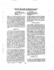
between the input and output blocks is necessary. Fortunately, XSG offers a simple interfacing using the predefined “gateway-in” and “gateway-out” blocks provided by the Xilinx blockset library. 3.2. General Structure of Wind-Solar System with XSG. To translate our system for the simulation with XSG, we need to change the specific blocks with an equivalent existing Xilinx library. The blockset in Figure 17 describes the global wind-solar system model designed with fuzzy logic controllers in a MATLAB/SIMULINK environment with XSG blocks. Adding the system generator and translating the two blocks, the fuzzy logic controllers of the solar and wind subsystems are necessary to pass the XSG simulation. We use the Xilinx library to change the MATLAB/SIMULINK component with adequate XSGs and to add gateway inputs and gateway outputs. The fuzzy toolbox does not exist in the XSG library, so we build it. It is composed of Min–Max inference rules, linguistic variables (PB, PS, ZE, NS, and NB) and defuzzification. We use a MUX from the Xilinx library to convert the output to numeric values with the gravity center method. The fuzzy built controller is integrated on wind and solar subsystems in the same way because it depends on E and dE. A description of the function of each subsystem (wind and solar fuzzy logic controllers) will be given in the following sections. 3.3. Hardware Architecture of Fuzzy Logic Controller. To build the solar fuzzy logic controller, we use the Xilinx library. As shown in Figure 18, we have two gateway inputs
International Journal of Photoenergy
1 E
2 dE
11
E
In Gateway in
dE
In
In1 In2 In3 In4 In5 In6 In7 In8 In9 In10
Out1 Out3 Out3 Out4 Out5 Out6 Out7 Out8 Out9 Out10
Gateway in1
Out1
In1
Out3
In2
Out3
In3
Out4
In4
Out5
In5
Decision-making logic
Fuzzification
d
Out Gateway out
1 d
Defuzzification
Figure 18: Architecture of solar fuzzy logic controller with XSG.
1
a
ln1 2
b
a
a-b
ln1
a
AddSub
0 Constant1
z−1 ab
Cast Convert1
Relational
Constant2
a b
Mult
a
a a+b
a
a-b b 2 ln2
z−3 a×b
z−1 a