Hardware implementation of GMDH-type artificial neural networks and ...

Hardware Implementation of GMDH-Type Artificial Neural Networks and its use to Predict Approximate Three-dimensional Structures of Proteins Andr´e L.S. Braga∗ , Janier Arias-Garcia∗ , Carlos Llanos∗ , M´arcio Dorn† , Alfredo Foltran‡ and Leandro S. Coelho§ ∗ Mechanical

Engineer Department. University of Brasilia. Brasilia – DF, Brazil of Informatics. Federal University of Rio Grande do Sul. Porto Alegre – RS, Brazil ‡ Vera Cruz Sistemas Computacionais. Brasilia – DF, Brazil § Produtronica Group. Pontifical Catholic University of Parana. Curitiba – PR, Brazil

† Institute

Abstract—Implementation of artificial neural networks in software on general purpose computer platforms are brought to an advanced level both in terms of performance and accuracy. Nonetheless, neural networks are not so easily applied in embedded systems, specially when the fully retraining of the network is required. This paper shows the results of the implementation of artificial neural networks based on the Group Method of Data Handling (GMDH) in reconfigurable hardware, both in the steps of training and running. A hardware architecture has been developed to be applied as a co-processing unit and an example application has been used to test its functionality. The application has been developed for the prediction of approximate 3-D structures of proteins. A set of experiments have been performed on a PC using the FPGA as a co-processor accessed through sockets over the TCP/IP protocol. The design flow employed demonstrated that it is possible to implement the network in hardware to be easily applied as an accelerator in embedded systems. The experiments show that the proposed implementation is effective in finding good quality solutions for the example problem. This work represents the early results of the novel technique of applying the GMDH algorithms in hardware for solving the problem of protein structures prediction.

I. I NTRODUCTION Artificial Neural Networks (ANNs) have been applied to solve a wide variety of problems where the complexity of the models makes them difficult or impractical to be solved by conventional techniques. Several FPGA implementations of ANNs have been recently proposed to tackle problems like dynamical systems identification [4], compression of digital images [26], [44], solving optimization problems [18], and so on. In general, those approaches point out the suitability of FPGAs for implementing intelligent system issues, which are characterized by their high complexity and, then, require a large computational effort to yield useful and practical results. Therefore, dedicated hardware for evolutionary and neural computation is becoming a key issue for designers [23]. One particularly problematic feature for developing ANNs in FPGAs is the design of the activation function [43], which bounds or modulate the outputs of neurons in many neural network models. The activation function can take many forms,

like, for example, a hyperbolic tangent (ϕ(v) = tanh(v)). There are several choices for designing these functions, like look-up tables (which consume a high number of memory blocks) or piece-wise linear approximation, i.e., the approximation of the output of the non-linear function by a sequence of linear functions outputs. Another important issue to be considered is the level of parallelism employed. Implementing many processing elements (neurons), require a great deal of hardware resources. Also, as the number of neurons grows, more interconnections between them are necessary, which also limits the size of the designs. Although the ANNs intrinsic parallelism is a motivation for implementing them in hardware, actually what is implied in this idea is that hardware implementations are going to be faster than software ones. Focus on parallelism is only justified when high performance is attained at reasonable cost [36]. For cost, though, it is possible to take into account factors other than just “price”. For embedded systems, for example, specially those which run under battery power, a key “cost” to be evaluated is the power consumption. Despite the fact that FPGA devices present a high static power consumption, i.e., power used just for keeping it turned it on, solutions based on custom hardware may deliver smaller power dissipation when performing intense calculations such as the ones present in the processing of ANNs [5]. Hardware implementation of GMDH-type Artificial Neural Networks is a somewhat straightforward task because their neurons dismiss the use of activation functions. Normally, each neuron contains a partial polynomial description of the system being modelled. In the basic form of the GMDH ANNs, partial descriptions are formed by second order polynomials. The use of polynomials is advantageous for hardware implementation purposes since they require simple mathematical operations: addition, subtraction, multiplication and non-negative integer exponents (which can be implemented by series of multiplications). The Group Method of Data Handling algorithm was developed in the late 1960s by Alexey G. Ivakhnenko, the method is one of the first approaches along the systematic design of

non-linear relationships. GMDH has been used with success in many fields such as data mining, knowledge discovery, prediction, modelling of complex systems, pattern recognition and optimization [21], [24], [1], [45] This article presents a hardware aided architecture to implements a GMDH-Type Artificial Neural Network. The project is focused on the development of a design flow that uses Matlab M-code training and execution functions and TCP/IP socket communication with the FPGA on which the designs are running. A set of libraries has been developed, allowing the GMDH-system (running in Matlab) to communicate with a GMDH neuron and with a Linear Systems Solving Module (LSSM) used to perform the Least Squares (LS) method (through Gaussian Elimination) for calculating the weights of the network neurons. Both the hardware GMDH neuron and the hardware LS module have been written in VHDL and tested on the FPGA device. In this work, the GMDH neuron was actually accessed through the TCP/IP connection while running on the FPGA, whereas the LSSM was running on the Mentor Graphics ModelSim simulation tool [34], to which the communication was abstracted through a transaction level modelling. TCP/IP communication has been achieved using a Xilinx MicroBlaze [51] soft-processor with Ethernet peripherals connected to it through a Processor Local Bus (PLB) [10]. The developed ANN was used to predict approximate 3-D structures of proteins as a case example for evaluating the system and the design flow. The network has been trained on-line using the Least Squares module and the weights obtained after training have been sent to the hardware-neuron through the socket connection. A set of experiments have been performed on a PC using the FPGA as a co-processor. The remaining of this text is structured as follows: Section II briefly introduces the basic concepts about proteins, about Group Method of Data Handling (GMDH), and about protein strictures prediction. Section III shows details of the implementation. Section IV reports several experiments and results, illustrating the effectiveness of the proposed method. Section V concludes and points out directions for further research. II. P RELIMINARIES A. GMDH principles The GMDH algorithms start by creating simple polynomials that roughly approximate the aimed systems and incrementally expand the complexity of those polynomials in order to create more accurate models. The polynomials usually follow the Kolmogorov-Gabor form, which is a discrete form of the Volterra functional as seen in Eq. 1 [31], [33].

φ = a0 + +

m X

ai xi +

m X m X

i=1 i=1 j=1 m X m X m X

aij xi xj +

aijk xi xj xk + · · ·

i=1 j=1 k=1

(1)

In order to create a full model of a system, several layers of partial descriptions are created to form a network inspired in the Multilayer Perceptron (MLP), which has the properties of a high order function as the one expressed in Eq. 1 [33], [20]. A typical partial description used in the GMDH neurons is given by Eq. 2, where xi and xj are the two inputs to the neuron and [a0 , ..., a5 ] are its coefficients. y = a0 + a1 xi + a2 xj + a3 x2i + a4 x2j + a5 xi xj

(2)

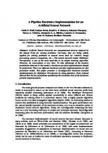
Figure 1 shows a possible architecture a GMDH-Type ANN after training. Each node contains one partial description and takes as inputs the outputs from two other nodes on the previous layer. GMDH networks must have one single output because all neurons are trained to approximate the same function: the desired output of the network. If the same inputs need to be used to yield more than one output, different GMDH ANNs must be created for each output.

Fig. 1. Possible architecture of a GMDH-type ANN after the training process. Squared nodes represent the inputs and circular nodes represent the neurons. The first layer (on the left) is the input layer, followed by four hidden layers and by an output layer which contains one single neuron.

Based on the number of inputs, the training algorithm instantiates a number of partial descriptions which constitute the neurons on the first hidden layer (in the remaining of this text, the term “first layer” designates the first hidden layer, the term “second layer”, designates the second hidden layer, and so on). The amount of partial descriptions on the first layer is defined by the number of combinations of the n inputs of the network taken two by two: m = C2n , where n is the number of inputs of the network. After training the first layer, a selection criterion is applied to exclude some neurons, keeping just those which better fit that criterion. A second layer is added after the selection of the best neurons on the first layer. The number of ˆ , where m ˆ is the number neurons on this new layer is p = C2m of neurons on the first layer after the selection process. The procedure of adding layers and selecting neurons is repeated until the last trained layer remain with one single neuron or when that layer does not improve the result of the network. If the layer remain with one single neuron, that node will be the output of the network; if the layer does not improve the performance, it is removed and the best neuron on the previous layer becomes the output of the network. Finally, all neurons from all previous layers which do not contribute to the value of the output neuron are removed [40], [12].

To determine the coefficients of the partial descriptions, a system of equations is created and solved for each one, following the Least Squares rule [20]. Each partial description is a function in the form of Eq. 2, which can be rewritten in the matrix form given by Eq. 3, where x represents the preprocessed inputs xi and xj of one neuron, expressed by x = [1, xi , xj , x2i , x2j , (xi xj )] [40], and a is a column vector with the coefficients to be calculated: a = [a0 , ..., a5 ]T . y = xa

From a structural point of view a protein or polypeptide is an ordered linear chain of amino acid residues chained by peptide bonds1 . The unique amino acid sequence of each protein molecule determine its three-dimensional (3-D) structure (native or functional state). This structure dictates the function of the protein on the cell: structural, catalysis in chemical reactions, transport, storage, regulation, recognition [28], [30].

(3)

Let X be a matrix containing all the preprocessed twoinputs samples to the neuron and b a column vector with all the desired outputs corresponding to the samples, as defined by Eq. 4 and Eq. 5.   1 xi (1) xj (1) x2i (1) x2j (1) χ(1)  1 xi (2) xj (2) x2i (2) x2j (2) χ(2)    (4) X= . .. .. .. .. ..  .  . . . . . .  1

xi (s)

xj (s)

x2i (s)

x2j (s)

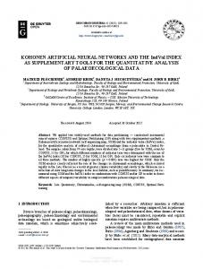
χ(s) Fig. 2. A model peptide illustrating the peptide bond, torsion angles φ, ψ, χ1 , χ2 , χ3 , χ4 . N is nitrogen, C and Cα are carbons and Ri is an arbitrary side-chain. Amino acid 1 represent an Arginine(ARG), amino acid 2 represent a Phenylamine (PHE).

where χ(t) = xi (t)xj (t) b = [b(1), b(2), b(3), · · · , b(s)]T

(5)

The relation among the weights a, the inputs and the outputs of the neuron is expressed by Eq. 6, where matrices b, X, and a have dimensions of N x 1, N x 6, and 6 x 1, respectively [20]. b = Xa

(6)

The normal equations are formed by pre-multiplying both sides by the transpose of X (Eq. 7). Matrix XT X has the dimensions of 6 x 6 and the solutions of the equations, shown in Eq. 8, are found by inverting this matrix [20]. XT b = (XT X)a

(7)

a = (XT X)−1 XT b

(8)

B. The protein structure prediction problem Proteins are long sequences of 20 different amino acids residues that, in physiological conditions, adopt a unique 3D structure [2]. That structure allows the protein to carry out its function in the cell [7]: enzymatic activity, storage and transport, antibodies and more. Tertiary protein structure prediction is one of the most important and unsolved problems in Structural Bioinformatics [16]. Efforts toward protein structures prediction have been made in many areas of computer science. For most of the past decade ANNs have produced accurate secondary structure predictions. In recent works, novel methods based on the Multilayer Perceptron [14] and on the GMDH algorithm [12] have been presented.

In nature there are 20 different amino acid residues. An amino acid residue is a molecule containing both amine (H3 N+ ), a carboxyl (COOH− ) functional group and a hydrogen (H) atom attached to a central carbon (Cα ). Each amino acid residue also has a R organic group (also known as sidechains) attached to its alpha carbon. This organic group gives the physiochemical proprieties of each amino acid residue. A peptide has three main-chain torsion angles: phi (φ), psi (ψ) and omega (ω) (Fig. 2). The bonds between N and Cα (phi), and between Cα and C (psi) are free to rotate. The set of torsion angles (main-chain ) of a polypeptide determine its conformation or fold [48], [28]. Protein structures can be studied in four levels: Primary structure: simply describes the sequence of amino acid residues in a linear order (N-Terminal → C-terminal). Secondary structure: is defined by the presence of hydrogen bond patterns between the backbone and the carboxyl groups in the polypeptide chain. There are two main secondary structures: α-helices [39] and β-sheets [38]. There is a third group of structures comprising coils and turns that are formed in regions where the polypeptide changes its directions, i.e., after a regular secondary structure in α-helix or β-sheet state. Tertiary structure: is the function state of a protein. It is formed by the grouping and interactions between α-helices and β-sheets determine the tertiary structure of the protein 1 Peptide bond. The covalent bond linking successive amino acids in the polypeptide chain.

Quaternary structure: is composed of groups of subunits in tertiary level. The prediction of the 3-D structure of proteins based only on the amino acid sequence (primary structure) is a challenging problem. Many computational methodologies, systems and algorithms have been proposed as a solution to the Protein Structure Prediction problem [22], [8], [49], [37], [42], [47]. Nevertheless, the problem still remains challenging because of the complexity and high dimensionality of a protein conformational search space [11], [17], [19], [29], [35]. The main challenge is to understand how the information encoded in the linear sequence of amino acid residues is translated into the 3-D structure, and from this acquired knowledge, to develop computational methodologies that can correctly predict the native structure of a protein molecule. III. M ATERIAL AND METHODS A. GMDH in hardware In this work, the two main basic operations of the GMDH algorithm have been implemented in VHDL: the neurons processing and the calculation of the coefficients of the neurons polynomials. A block diagram of the GMDH neuron in hardware is shown in Fig. 3. On the left of the diagram, two FIFO units are shown. They are responsible for receiving the neurons weights and the input values. The FIFO controllers connected to the admission FIFOs are responsible for reading and parallelizing the entering data according to the requisites of the processing element and for storing them in the appropriate registers inside the Register Bank. Since the GMDH polynomial has six terms (see Eq. 2), six values are read by the Weights FIFO Controller and stored in the Register Bank. For the neuron inputs, the Inputs FIFO Controller reads two values from the Inputs FIFO and bank them.

Weights FIFO

FIFO Controller

FIFO Controller

+

Register Bank Inputs FIFO

Outputs FIFO

FIFO Controller

x FSM GMDH Neuron

Fig. 3.

Block diagram of the GMDH neuron in hardware.

A finite states machine (FSM), shown in the lower part of Fig. 3, is responsible for controlling the reading process as well as all the other steps of the neuron operations. As soon as the first terms are made available in the Register Bank, the FSM switches the multiplexers which are connected to the adder and to the multiplier. These are pipelined floating point arithmetic units which have been built with Xilinx CORE Generator (version 13.4) [52]. The FIFO units are also implemented with Core Generator.

All units in the design work in parallel, thus the mathematical operations can start before all data are present in the Register Bank. Taking into account the latency of the floating point units, the FSM feeds the next data available at each clock cycle. The arithmetic outputs are stored back in the Register Bank and, when the calculations are finished, the neuron output is delivered to another FIFO Controller (Fig. 3, on the right) which, in turn, send it to the Outputs FIFO. The FSM is implemented in a way that the neuron weights and the inputs to the neuron can be delivered on different times. Whenever a group of six coefficients and a group of two inputs are available, the neuron can start the calculations. If no other coefficient is sent to the Weights FIFO, the neuron keeps reading and processing the inputs. The Inputs FIFO has 256 positions, allowing the processing of 128 outputs of the neuron at one round of communication with the FPGA. B. Software-hardware Co-verification The designs implemented in this work have been tested using a design flow which employs TCP/IP socket communication between the PC and the FPGA where the GMDH neuron and the LSSM are programmed. While the GMDH neuron was actually programmed on the FPGA, the LSSM ran on the ModelSim simulation tool, to which the communication was abstracted through a transaction level modeling. This abstraction was reached through an M-code library which deals with the details of the communication with the designs, thus isolating the GMDH training and execution algorithms from the complexity involved in those operations. To perform the TCP/IP communication, a MicroBlaze softprocessor was employed. The GMDH neuron and the LSSM have ben used as peripherals to the processor, attached to a PLB bus, as depicted in Fig. 4. This is possible through the use of VHDL wrappers which encapsulate user logic as a MicroBlaze peripheral. The process creating such peripherals is assisted by the Xilinx Platform Studio integrated environment [53]. The design shown in Fig. 4, employing the GMDH neuron, has been tested on a XUPV5-LX110T development kit which contains a Xilinx Virtex 5 vlx110T device [54]. Since the LSSM peripheral was not fully functional at the time the experiments presented in this work have been performed, it was simulated using ModelSim instead of actually run on the FPGA. A software tool have been developed to train and execute GMDH ANNs [6], [12]. This tool have been adapted to be able to employ the software-hardware co-verification through the socket communication. The GMDH software operate as if it was not relying on the co-verification design, but when the neuron execution method is called in Matlab, data are transferred to the FPGA through the socket connection and the results are retrieved, when they’re ready, through the same channel. On the other hand, when the training methods require the calculation of the neurons weights, the M-code libraries transparently call the the Least Squares procedure performed by the LSSM being simulated on the ModelSim tool.

When the LSSM finishes the Gaussian Elimination, its FSM starts copying the last column of the matrix stored in the internal RAM to the output FIFO. Details about the LSSM, for example, on the hardware optimizations obtained, can be found in Arias-Garcia et. al [3].

Matrix Matrix LSSM Inverter Inverter Peripheral Peripheral Peripheral

DDR2 DDR2 Controller Controller

GMDH GMDH Neuron Neuron Peripheral Peripheral

Timer Timer Hard Hard Ethernet Ethernet MAC MAC

PLB BUS BUS PLB

Board DDR2 SDRAM

MicroBlaze MicroBlaze

Interrupt Interrupt Controller Controller

FPGA Design Board Board Phy Phy Device Device

Row FIFO

FIFO Controller

Row FIFO

FIFO Controller

Row FIFO

FIFO Controller

Row FIFO

FIFO Controller

Row FIFO

FIFO Controller

Row FIFO

FIFO Controller

Gaussian Elimination Unit - GEU RAM FIFO Controller

Output FIFO

FSM Linear Systems Solving Module – LSSM

Fig. 4. Design of the GMDH neuron and the LSSM as peripherals of a MicroBlaze soft-processor attached to a PLB bus.

Fig. 5. LSSM - Linear Systems Solving Module used to accelerate the Least Squares method

C. Linear systems solving module (LSSM) The LSSM was developed for solving linear systems in general using the Gaussian Elimination process. To fit the requirements of the project presented in this work, it was adapted to calculate the coefficients of the GMDH neurons, i.e., to solve systems with 6 equations and 6 unknowns. Gaussian Elimination is suitable for the GMDH method, especially in consideration to the wide variety of problems which can be presented to the networks. According to the availability of hardware components, different methods can be applied as well. Figure 5 shows that the LSSM comprises: (a) a RAM block where the elements of the matrix are stored; (b) the Gaussian Elimination Unit (GEU) which iteratively reads from and writes to the RAM block until all the equation unknowns are found; (c) a set of FIFO controllers, responsible for the connection with the 6 Row FIFOs and with the Outputs FIFO and; (d) a Finite States Machine (FSM) responsible for the coordination of the data transfers among the other blocks. The coefficients of one neuron are calculated using Eq. 8. The LSSM performs this calculation taking as input the matrix formed by Eq. 9. [M, p] is a 6 x 7 matrix which is sent to the module.   [M, p] = (XT X), XT b

(9)

Internally, a 6 x 6 Identity matrix in incorporated to the stored values (See Eq. 10). After performing the Gaussian Elimination method, which is carried out through simple operations like multiplications and data moving, the internal memory holds the values presented in Eq. 11, where I and M−1 are 6 x 6 matrices and a is a 6 x 1 vector containing the coefficients which solve the system of linear equations. [M, I, p]   I, M−1 , a

(10) (11)

D. Protein structural patterns acquisition In order to reduce the complexity and the high dimensionality of the conformational search space inherent to ab initio2 protein structure prediction methods, information about structural motifs found in known protein structures can be used to construct approximated conformations [15], [13]. This predicted approximate 3-D structure is expected to be good enough to be further refined by means of molecular mechanics methods such as Molecular Dynamics simulations [50], [41], [25]. In this work we use an adapted version of the A3N (Artificial Neural Network N-gram-based) [14] method in order to acquire structural information of experimentally determined 3-D protein structures from the Protein Data Bank (PDB). A3N fragments the target amino acid sequence in consecutive fragments with size five and search the PDB in order to find protein structures with similar sequences. A set of templates fragments are obtained from each target fragment. The protein secondary structure of each template fragment and the PHI and PSI torsion angles values of its central amino acid residue calculated using Promotif. The pairs of torsion angles φ and ψ of each template fragment are clustered using the EM clustering algorithm. Training patterns are built using the secondary structure information, the amino acid type of the template fragment and the cluster which the template fragment belongs after the clustering procedure. A training pattern has the form:[ss1 , ss2 , ss3 , ss4 , ss5 , a1 , a2 , a3 , a4 , a5 :t, where ssi represents the secondary structure state of the ith amino acid residue, ai represents the ith amino acid residue and t represents the cluster identifier. The secondary structure and the amino acid residue information are used as the input object and the cluster number as a desired output value to the ANN 2 Ab initio method are founded on thermodynamics and based on the fact that the native structure of a protein corresponds to the global minimum of its free energy.

being training. A complete description of the A3N algorithm can be found in Dorn and Norberto de Souza [14]. In order to build the unknown sample, the secondary structure of the target amino acid sequence is predicted using SCRATCH secondary prediction server [46]. The fragment composed of amino acid residues is combined with its corresponding secondary structure fragment in order to build the target patterns. This patterns are afterwards submitted to its ANNs in order to predict its cluster. IV. E XPERIMENTAL RESULTS The hardware implementation of the GMDH model described in this paper was applied to predict the 3-D structure of the protein with PDB ID = 1WQC [9]. The Om-toxin of the scorpion Opisthacanthus madagascariensi (PDB ID: 1WQC) is a polypeptide composed by 26 amino acid residues (DPCYEVCLQQHGNVKECEEACKHPVE) known to be arranged as two α-helices connected by a turn, a structural motif known as an α-helical hairpin. The target amino acid sequence was submited to the A3N method in order to acquire structural patterns from the PDB. GMDH ANN are built for each target fragment an templates from PDB are used to train them. The experiments have been composed of ten different trials in which templates have been extracted from the Protein Data Bank PDB and used to train the GMDH ANNs. At each trial, the templates were shuffled and then divided in two groups: (a) the training group and (b) the selection group, as it is required by the GMDH networks. For comparison purposes we test the same protein target sequence of the protein 1WQC in our software implementation of the GMDH ANN. For structural and biochemical analysis we selected the obtained results of the predicted structures woth the lowest RMSD value after ten trials. Structural quality measurements have been made in terms of the root mean standard deviations (RMSD) between the positions of the atoms in the original and estimated structures calculated using Eq. 12. In this equation, rai and rbi are vectors representing the positions of the same atom i in each of two structures, a and b respectively, and where the structures a and b are optimally superimposed. The RMSD value calculated between two structures is obtained using the PROFIT software [32]. Table I - column 2, presents the RMSD values obtained for the target amino acid sequence using the software and the hardware implementation of the GMDH ANNs. v ! u n u X krai − rbi k2 /n (12) RMSD(a, b) = t i=1

Figure 6 shows the ribbon representations of the experimental (A - gray) and predicted structures (B software implementation - magenta and C hardware implementation - magenta). By visual inspection, it is noticeble that the individual helices and the secondary structures are well formed in the software and the hardware implementation of the GMDH model. In oder to analyze the secondary structure arrangement of the predicted structures (Figure 6 B-C - magenta) we run the

Fig. 6. Ribbon representation of the experimental (gray) and predicted structures (magenta). The Cα of the experimental and predicted structures are fitted. (A) Experimental 3-D structure of protein with PDB ID = 1WQC, (B) Experimental and predicted 3-D structure of protein with PDB ID = 1WQC using the software implementation of the GMDH model, (C) Experimental and predicted 3-D structure of protein with PDB ID = 1WQC usgin the hardware implementation of the GMDH model. Amino acid side chains are not shown for clarity. Graphics were generated by . CHIMERA TABLE I Cα ROOT MEAN SQUARE DEVIATION (RMSD) OF PREDICTED STRUCTURES WITH RESPECT TO THEIR EXPERIMENTAL STRUCTURES AND ANALYSIS OF THE SECONDARY STRUCTURE ARRANGEMENT OF THE PREDICTED APPROXIMATE CONFORMATIONS . -E DENOTES THE EXPERIMENTAL STRUCTURE . -S DENOTES THE PREDICTED STRUCTURES USING THE SOFTWARE IMPLEMENTATION OF THE GMDH NEURAL MODEL . -H DENOTES THE PREDICTED STRUCTURES USING THE HARDWARE IMPLEMENTATION OF THE GMDH MODEL .

PDB ID 1WQC-E 1WQC-S 1WQC-H

˚ RMSD (A) 00.0 02.8 02.6

Strand 00.0% 00.0% 00.0%

α-helix 65.4% 61.5% 65.4%

310 00.0% 00.0% 00.0%

Other 34.6% 38.5% 34.6%

PROMOTIF tool. Table I shows the number (%) of amino acid residues that occur in one of four conformational states (Regular conformational state: β-sheet, α-helix, 310 -helix and others (coil or loop regions)). We observe that the secondary structure formation of the predicted structures by both hardware and software implementation of the GMDH ANN are closely related to their experimental structures. We run the PROCHECK software [27] in order to obtain information about the distribution of the amino acid residues in the Ramachandran Plot. These results are illustrate in Fig. 7 and summarized in Table II. Both obtained results with the hardware and software implementation of the GMDH model present more than 90% of the amino acid residues in the most favorable regions of the Ramachandran Plot. A high amount of amino acid residues in a favorable region means that the structures have a small number of bad contacts. The shorter differences in the number of amino acid residues between the predicted and the experimental structures occur in the regions where the full structures change their conformational state (α- helix or β-sheet regions to coil or loop region). Nevertheless, this short distortion can be corrected through mechanical methods that can simulate and optimize the interactions between all atoms and allow hydrogen bonds formation in order to stabilize those regions [13].

Fig. 7. Ramachandran Plot of the experimental and predicted structures. (A) Ramachandran plot of the experimental protein with PDB ID 1WQC. (B) Ramachandran plot of the predicted 3-D structure of the protein with PDB ID 1WQC using the software implementation of the GMDH model. (C) Ramachandran plot of the predicted 3-D structure of the protein with PDB ID 1WQC using the hardware implementation of the GMDH model. Graphics representations were generated by PROCHECK.

TABLE II N UMERICAL R AMACHANDRAN PLOT VALUES FOR THE EXPERIMENTAL AND PREDICTED CONFORMATIONS . -E DENOTES THE EXPERIMENTAL STRUCTURE . -S DENOTES THE PREDICTED STRUCTURES USING THE SOFTWARE IMPLEMENTATION OF THE GMDH NEURAL MODEL . -H DENOTES THE PREDICTED STRUCTURES USING THE HARDWARE IMPLEMENTATION OF THE GMDH MODEL .

PDB ID 1WQC-E 1WQC-S 1WQC-H

Most favorable 90.5% 90.5% 95.2%

Additional allowed 00.0% 04.8% 00.0%

Generously allowed 09.5% 04.8% 04.8%

Disallowed 00.0% 00.0% 00.0%

V. C ONCLUSIONS AND FURTHER WORK This work demonstrated the application of hardware acceleration of GMDH artificial neural networks using VHDL based modules for the most computer intensive operations of the network algorithm, namely: (a) the computation of the polynomial expressions present in the neurons and; (b) the fulfil of the Least Squares method for calculating the polynomial coefficients during the training process. Two hardware modules have been developed using VHDL code: the GMDH neuron and the Linear Systems Solver Module. The designs have been synthesized and tested on a Xilinx Virtex 5 vlx110T device. A GMDH application written in M-code is used to train and to run GMDH ANNs. A running strategy have been developed in order to evaluate the functionality of the VHDL designs. Through the use of a set of M-functions which abstract the communication with the platform where the designs are being carried or simulated, the GMDH library could use the functionality implemented by the hardware designs. The abstraction functions have been employed to communicate with the modules both in simulation mode, using the Mentor Graphics ModelSim simulation tool, and on the FPGA, through socket connections over TCP/IP. The GMDH neuron was implemented as a peripheral connected to a PLB bus on which a MicroBlaze soft-processor was attached. The MicroBlaze was used to carry out the socket

connection and to transfer the data to and from the GMDH Neuron. The matrix inverter code was evaluated only using the simulation approach. In order to examine the suitability of the design flow, an example application have been developed. The designs have been used to predict approximate structures of protein sequences. Results demonstrated that the GMDH based method using FPGA acceleration is effective for tackling the problem of prediction of 3-D protein sequences structures. Despite the fact that general purpose computers have enough power to carry out all the phases of the GMDH algorithms, the acceleration achieved by the hardware modules can be a key feature for the employment of artificial neural networks in embedded applications. Early evaluations suggest that one single GMDH neuron, which takes only 3% of the resources offered by the FPGA employed in this work (using the current developed code), can achieve up to 89 KFLOPS/MHz. The next steps on the development of the design flow is to implement the LSSM as a PLB peripheral and evaluate the hardware accelerator in embedded applications. Possible paths are to instantiate more GMDH neurons as peripherals running in parallel and to bring more pieces of the GMDH algorithm to the micro-controllers level or even to the hardware level. With the results obtained in this work, it is proved that the hardware acceleration of the GMDH algorithm is possible and functional. ACKNOWLEDGMENT This work was supported by grants from the Brazilian scientific funding agencies MCT/CNPq and MCT/CAPES. The authors would like to thank the Xilinx University Program and the Mentor Graphics Higher Education Program for the software licences provided, and the Institut f¨ur Technik der Informationsverarbeitung - ITIV, from the Karlsruhe Institute of Technlogy - KIT, Karlsruhe, Germany, for the support on the development of the GMDH library in the form advice, infrastructure and software licenses and for providing the development kit board on which the experiments have been

performed. R EFERENCES [1] R. Abdel-Aal, M. Elhadidy, and S. Shaahid. Modeling and forecasting the mean hourly wind speed time series using gmdh-based abductive networks. Renewable Energy, 34(7):1686–1699, 2009. [2] C. Anfinsen, E. Haber, M. Sela, and F. H. J. White. The kinetics of formation of native ribonuclease during oxidation of the reduced polypeptide chain. Proc. Natl. Acad. Sci. U.S.A., 47:1309, 1961. [3] J. Arias-Garcia, C. Llanos, M. Ayala-Rincon, and R. Jacobi. A fast and low cost architecture developed in fpgas for solving systems of linear equations. In Circuits and Systems (LASCAS), 2012 IEEE Third Latin American Symposium on, pages 1–4, 29 2012-march 2 2012. [4] M. Atencia, H. Boumeridja, G. Joya, F. Garc´ıa-Lagos, and F. Sandoval. Fpga implementation of a systems identification module based upon hopfield networks. Neurocomputing, 70(16–18):2828–2835, 2007. [5] A. Braga, C. Llanos, D. Go andhringer, J. Obie, J. Becker, and M. Hubner. Performance, accuracy, power consumption and resource utilization analysis for hardware / software realized artificial neural networks. In Bio-Inspired Computing: Theories and Applications (BICTA), 2010 IEEE Fifth International Conference on, pages 1629–1636, sept. 2010. [6] A. L. S. Braga. Gmdh-t-ann - gmdh type artificial neural network, June 2011. [7] C. Branden and J. Tooze. Introduction to protein structure. Garlang Publishing Inc., New York, 2 edition, 1998. [8] S. H. Bryant and S. Altschul. Statistics of sequence-structure threading. Curr. Opin. Struct. Biol., 5(2):236, 1995. [9] B. Chagot, C. Pimentel, L. Dai, J. Pil, J. Tytgat, T. Nakajima, G. Corzo, H. Darbon, and G. Ferrat. An unusual fold for potassium channel blockers: Nmr structure of three toxins from the scorpion opisthacanthus madagascariensis. Biochem. J., 388:263–271, 2005. [10] I. Corporation. 32-bit Processor Local Bus Architecture Specications Version 2.9. [11] P. Crescenzi, D. Goldman, C. Papadimitriou, A. Piccolboni, and M. Yannakakis. On the complexity of protein folding. J. Comput. Biol., 5(3):423, 1998. [12] M. Dorn, A. L. Braga, C. H. Llanos, and L. dos S. Coelho. A gmdh polynomial neural network-based method to predict approximate three-dimensional structures of polypeptides. Expert Systems with Applications, (0):–, 2012. [13] M. Dorn, A. Breda, and O. Norberto de Souza. A hybrid method for the protein structure prediction problem. Lect. Notes Bioinf., 5167:47, 2008. [14] M. Dorn and O. Norberto de Souza. A3n: an artificial neural network n-gram-based method to approximate 3-d polypeptides structure prediction. Expert Syst. Appl., 37(12):7497, 2010. [15] H. Fan and A. Mark. Refinement of homology-based protein structures by molecular dynamics simulation techniques. Protein Sci., 13:211–220, 2004. [16] C. Floudas, H. Fung, S. McAllister, M. Moennigmann, and R. Rajgaria. Advances in protein structure prediction and de novo protein design: A review. Chem. Eng. Sci., 61(3):966, 2006. [17] A. S. Fraenkel. Complexity of protein folding. Bull. Math. Biol., 55(6):1199, 1993. [18] G. Grossi and F. Pedersini. Fpga implementation of a stochastic neural network for monotonic pseudo-boolean optimization. Neural Networks, 21(6):872–879, 2008. [19] W. Hart and S. Istrail. Robust proofs of np-hardness for protein folding: general lattices and energy potentials. J. Comput. Biol., 4(1):1, 1997. [20] A. G. Ivakhnenko. Polynomial theory of complex systems. Systems, Man and Cybernetics, IEEE Transactions on, 1(4):364–378, oct. 1971. [21] A. G. Ivakhnenko and G. A. Ivakhnenko. The review of problemas solvable with algorithms of the Group Method of Data Handling (GMDH). Pattern Recognition and Image Analysis, 5(4):527–535, 1995. [22] D. Jones, W. Taylor, and J. Thornton. A new approach to protein fold recognition. Nature, 358(6381):86, 1992. [23] S. Kilts. Advanced FPGA Design: Architecture, Implementation, and Optimization. Wiley-IEEE Press, 1 edition, Aug. 2007. [24] T. Kondo and A. Pandya. Gmdh-type neural networks with a feedback loop and their application to the identification of large-spatial air pollution patterns. In SICE 2000. Proceedings of the 39th SICE Annual Conference. International Session Papers, pages 19–24, 2000.

[25] J. R. Koza. Molecular dynamics simulations: Elementary methods. John Wiley and Sons, Inc., New York, 1 edition, 1992. [26] W. Kurdthongmee. A novel hardware-oriented kohonen som image compression algorithm and its fpga implementation. J. Syst. Archit., 54(10):983–994, Oct. 2008. [27] R. Laskowski, M. MacArthur, D. Moss, and J. Thornton. Procheck: a program to check the stereochemical quality of protein structures. J. Appl. Crystallogr., 26(2):283–291, 1993. [28] A. M. Lesk. Introduction to Bioinformatics. Oxford University Press Inc., New York, 1 edition, 2002. [29] C. Levinthal. Are there pathways for protein folding? J. Chim. Phys. Phys.-Chim. Biol., 65(1):44, 1968. [30] H. Lodish, A. Berk, P. Matsudaira, C. A. Kaiser, M. Krieger, and M. Scott. Molecular Cell Biology. Scientific American Books, W.H. Freeman, New York, 5 edition, 1990. [31] H. R. Madala and A. G. Ivakhnenko. Inductive Learning Algorithms for Complex Systems Modeling, chapter 3. CRC Press, Boca Raton, Florida, 1994. [32] A. C. R. Martin. Profit web page, 2012. [33] R. K. Mehra. Group method of data handling (gmdh): Review and experience. In Decision and Control including the 16th Symposium on Adaptive Processes and A Special Symposium on Fuzzy Set Theory and Applications, 1977 IEEE Conference on, volume 16, pages 29–34, dec. 1977. [34] Mentor Graphics. Modelsim - advanced simulation and debugging, May 2012. [35] J. Ngo, J. Marks, and M. Karplus. The protein folding problem and tertiary structure prediction. In K. Merz Jr and S. Grand, editors, Computational complexity, protein structure prediction and the Levinthal Paradox, page 435. Birkhauser, Boston, 1997. [36] A. R. Omondi and J. C. RAJAPAKSE. ASIC vs. FPGA neurocomputers, chapter 1, page 9. Springer, 2006. [37] D. Osguthorpe. Ab initio protein folding. Curr. Opin. Struct. Biol., 10(2):146, 2000. [38] L. Pauling and R. Corey. The pleated sheet, a new layer configuration of polypeptide chains. Proc. Natl. Acad. Sci. U.S.A., 37(5):251, 1951. [39] L. Pauling, R. Corey, and H. Branson. The structure of proteins: two hydrogen-bonded helical configurations of the polypeptide chain. Proc. Natl. Acad. Sci. U.S.A., 37(4):205, 1951. [40] D. T. Pham and X. Liu. Modelling and prediction using GMDH networks of Adalines with nonlinear preprocessors. International Journal of Systems Science, 25:1743–1759, 1994. [41] D. C. Rapaport. The art of molecular dynamics simulation. Cambridge University Press, Cambridge, 2 edition, 2004. [42] C. Rohl, C. Strauss, K. Misura, and D. Baker. Protein structure prediction using rosetta. Methods Enzymol., 383(2):66, 2004. [43] V. Saichand, D. Nirmala, S. Arumugam, and N. Mohankumar. Fpga realization of activation function for artificial neural networks. In Intelligent Systems Design and Applications, 2008. ISDA ’08. Eighth International Conference on, volume 3, pages 159–164, nov. 2008. [44] S. Saif, H. M. Abbas, S. M. Nassar, and A. A. Wahdan. An fpga implementation of a neural optimization of block truncation coding for image/video compression. Microprocess. Microsyst., 31(8):477–486, Dec. 2007. [45] A. Sakaguchi, T. Yamamoto, K. Fujii, and Y. Monden. Evolutionary gmdh-based identification for nonlinear systems. In Systems, Man and Cybernetics, 2004 IEEE International Conference on, volume 6, pages 5812–5817 vol.6, oct. 2004. [46] Scratch. Scratch protein preditor webpage, Jan. 2012. [47] R. Srinivasan and G. Rose. Linus - a hierarchic procedure to predict the fold of a protein. Proteins: Struct., Funct., Bioinf., 22(2):81, 1995. [48] A. Tramontano. Protein structure prediction. John Wiley and Sons, Inc., Weinheim, 1 edition, 2006. [49] M. Turcotte, S. Muggleton, and M. Sternberg. Application of inductive logic programming to discover rules governing the three-dimensional topology of protein structure. Springer, Madison, July 1998. [50] W. van Gunsteren and H. Berendsen. Computer simulation of molecular dynamics: methodology, applications, and perspectives in chemistry. Angew. Chem., Int. Ed. Engl., 29(9):992, 1990. [51] Xilinx Inc. Microblaze soft processor core. [52] Xilinx Inc. Xilinx core generator system, May 2012. [53] Xilinx Inc. Xilinx platform studio, May 2012. [54] Xilinx Inc. Xilinx University Program XUPV5-LX110T Development System, Apr. 2012.