Helical States in Curved Bilayer Graphene

Helical States in Curved Bilayer Graphene Jelena Klinovaja, Gerson J. Ferreira, and Daniel Loss

arXiv:1208.2601v1 [cond-mat.mes-hall] 13 Aug 2012

Department of Physics, University of Basel, Klingelbergstrasse 82, CH-4056 Basel, Switzerland (Dated: August 14, 2012) We study spin effects of quantum wires formed in bilayer graphene by electrostatic confinement. With a proper choice of the confinement direction, we show that in the presence of magnetic field, spin-orbit interaction induced by curvature, and intervalley scattering, bound states emerge that are helical. The localization length of these helical states can be modulated by the gate voltage which enables the control of the tunnel coupling between two parallel wires. Allowing for proximity effect via an s-wave superconductor, we show that the helical modes give rise to Majorana fermions in bilayer graphene. PACS numbers: 73.22.Pr, 75.70.Tj, 73.63.Fg, 72.25.-b

Introduction. Graphene and its derivatives [1–4], such as bilayer graphene (BLG) and carbon nanotubes (CNT), have attracted wide interest due to its peculiar bandstructure with low energy excitations described by Diraclike Hamiltonians. Moreover, these materials are usually placed on substrates, which allows high control of its geometry, doping, and placement of metallic gates [5–9]. Topological insulators were predicted for graphene [10], but later it was found that the intrinsic spin-orbit interaction (SOI) is too weak [11, 12]. For BLG, first-principle calculations also show weak SOI [13, 14]. In an other proposal, topologically confined bound states were predicted to occur in BLG where a gap and band inversion is enforced by gates [15]. Quite remarkably, these states are localized in the region where the voltage changes sign, are independent of the edges of the sample, and propagate along the direction of the gates, thus forming effectively a quantum wire [15–17]. At any fixed energy, the spectrum inside the gap is topologically equivalent to four Dirac cones, each cone consisting of a pair of states with opposite momenta. The spin degrees of freedom in such BLG wires, however, have not been addressed yet. It is the goal of this work to include them and to show that they give rise to striking effects. In particular, we uncover a mechanism enabling helical modes propagating along the wires. In analogy to Rashba nanowires [18], topological insulators [19], and CNTs [20, 21], such modes provide the platform for a number of interesting effects such as spinfiltering and Majorana fermions [22]. Here, the SOI plays a critical role, and in order to substantially enhance it, we consider a BLG sheet with local curvature as shown in Fig. 1. Two pairs of top and bottom gates define the direction of the quantum wire which is chosen in such a way that it corresponds to a ‘semi-CNT’ of zigzag type. In this geometry, the energy levels of the mid-gap states cross in the center of the Brillouin zone. A magnetic field transverse to the wire in combination with intervalley scattering leads to an opening of a gap, 2∆g , between two Kramers partners at zero momentum, see Fig. 2. As a result, the number of Dirac cones changes from even

FIG. 1. A bilayer graphene (BLG) sheet with a fold at x = 0 along the z-axis is placed between two pairs of gates that are set to opposite polarities ±V0 /2, inducing the bulk gap. There are mid-gap bound states, localized in transverse x-direction around x = 0. At the same time, they freely propagate along the z-direction, forming an effective quantum wire [15]. An externally applied magnetic field B = Bex0 breaks timereversal symmetry. The spin-orbit interaction β is induced by the curvature of the wire, which is characterized by the radius R. In the insets we show the BLG structure in momentum (left) and real (right) space for a chosen chirality θ = 0. The edges of the BLG sheet can be arbitrary.

(four) to odd (three), and the wire becomes helical with opposite spins being transported into opposite directions. In the following we derive the spectrum and its characteristics analytically and confirm these results by independent numerics. We also address the physics of Majorana fermions which emerge when the wire is in proximity contact to an s-wave superconductor. Curved bilayer graphene with SOI. We consider a gated curved bilayer graphene with a magnetic field B (along the x0 -axis) applied perpendicular to the direction of the fold (along the z-axis), see Fig. 1. We begin with a description of the bilayer graphene in the framework of the tight-binding model [3, 4]. Each layer is a honeycomb lattice composed of two types of non-equivalent atoms A1 (A2 ) and B1 (B2 ) and defined by two lattice vectors a1 and a2 . We focus here on AB stacked bilayer, in which two layers are coupled only via atoms A2

2 and B1 (see Fig. 1) with a hopping matrix element t⊥ (t⊥ ≈ 0.34 eV). By analogy with CNTs [3], we introduce a chiral angle θ as the angle between a1 and the x-axis. The low-enegy physics is determined by two valleys defined as K = −K0 = (4π/3a)(cos θ, sin θ), where a = |a1 |. The corresponding Hamiltonian in momentum space is written as H0 = ~υF (kx σ1 + τ3 kz σ2 ) +

t⊥ (σ1 η1 + σ2 η2 ) − V η3 , (1) 2

where the Pauli matrices σi (ηi ) act in the sublattice (layer) space, and the Pauli √ matrices τi act in the valley space. Here, υF = 3ta/2~ is the Fermi velocity (υF ≈ 108 cm/s), with t ≈ 2.7 eV being the intralayer hopping matrix element. The kx (kz ) is the transversal (longitudinal) momentum calculated from the points K and K0 . The potential difference between the layers opens up a gap 2|V | in the bulk spectrum, while a spatial modulation, i.e. V → V (x), breaks the translation invariance along the x-direction, thus only the total lon(0) gitudinal momentum Kz + kz remains a good quantum number.

E (meV)

29.2

29.1

29

28.9 -0.1

2∆g ↑K ↓K ↑K′ ↓K′

-20

2β

-10

0

10

20

V0

-0.05 kz

0 (10−2

0.05

0.1

nm−1 )

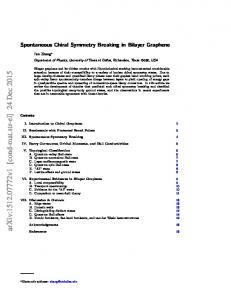
FIG. 2. The spectrum of the BLG structure for V0 /2 = 50 meV and chirality θ = 0. The green area in the inset corresponds to the bulk spectrum. The mid-gap bound states for valleys K (full line) and K 0 (dashed line) have opposite velocities. The main figure shows the details of K-K 0 crossing region (shaded region in the inset). The curvature induced SOI shifts spin-up and spin-down levels in opposite directions by the SOI parameter β. A magnetic field B assisted by intervalley scattering ∆KK 0 results in the anti-crossing gap 2∆g of two Kramers partners at kz = 0. If the chemical potential µ is √ tuned inside the gap [shaded area with µ ≈ (V0 /2 2)±β], the system is equivalent to three Dirac cones (only one is shown in the main Figure), resulting in the helical mode regime. Here, β ≈ 60 µeV (R = 5 nm), ∆KK 0 = 30 µeV, and ∆Z = 30 µeV, so the opened gap is 2∆g ≈ 30 µeV≈ 300 mK.

The Hamiltonain H0 can be simplified for small voltages, |V |  t⊥ , by integrating out the A2 and B1 degrees of freedom, which correspond to much higher energies

E ≈ t⊥ . The effective Hamiltonian becomes 2 2 2 2
˜ 0 = −V γ3 − ~ υF kx2 − kz2 γ1 − 2~ υF kx kz τ3 γ2 , (2) H t⊥ t⊥

where the Pauli matrices γi act in the space of A1 and B2 atoms. If the voltage changes sign at x = 0 [for example, V (x) = −V (−x)], this results in the closing and reopening of the gap. As a consequence, bound states, localized around x = 0, emerge within the bulk gap [15]. ˜ 0 are characterized by kz and the The eigenstates of H valley degree of freedom τ = ±1. For a step-like kink potential V (x) = (V0 /2) sgn(x) the energy spectrum is shown in the inset of Fig. 2. Now we include spin and aim at the realization of helical modes in BLG, which requires an analysis of the spin-full mid-gap states. At any fixed energy in the bulk gap, there are 2 × 4 states, where the factor 2 arises from spin-degeneracy. This means that the spectrum is topologically equivalent to four Dirac cones, each cone consisting of a pair of states with opposite momenta. On the other hand, helical modes are typical for systems with an odd number of Dirac cones. To effectively eliminate one Dirac cone at given chemical potential, the spindegeneracy should be lifted by a magnetic field B, giving rise to a new gap. Obviously, the opening of such a gap is possible only if there is level crossing in the system. The spectrum of the mid-gap states has support around K and K 0 . Therefore, if these points, projected onto the kz -axis, are separated from each other, no crossing can occur. We thus see that the chiral angle θ is of a crucial importance for our purpose and the optimal choice is θ = 0 (or very close to it). In this case, Kz = K0z = 0, and the level crossing occurs in the center of the Brillouin zone, at kz = 0, see inset of Fig. 2. We emphasize that in contrast to nanoribbons [16] the form of the edges of the BLG sheet does not matter provided the distance between edges and wire-axis is much larger than the localization length ξ of the bound state. Next, we allow also for spin-orbit interaction in our model. While the intrinsic SOI is known to be weak for graphene [11, 12], the strength of SOI in CNT is enhanced by curvature [20, 23–25]. To take advantage of this enhancement, we consider a folded BLG which is analogous to a zigzag semi-CNT with θ = 0. All SOI terms that can be generated in second-order perturbation theory are listed in Table I of Refs. [20, 25]. From these terms only Hso = βτ3 sz is relevant for our problem; first, it is the largest term by magnitude, and second, it is the only term which acts directly in the A1 -B2 space. Here, si is the Pauli matrix acting on the electron spin, and i = x, y, z. The value of the effective SOI strength β depends on the curvature, defined by the radius R, and is given by β ≈ 0.31 meV/R[nm] [20]. In the presence of SOI, the states can still be characterized by the momentum kz , valley index τ = ±1, and spin projection s = ±1 on the z-axis. The spec-

3 ˜ 0 + Hso can be obtained from the one of H ˜0 trum of H by simply shifting E → E − βτ s. This transformation goes through the calculation straightforwardly, and the spectrum in the presence of the SOI becomes (~υF kz 4t⊥

V0 + √ 2 2

V0 ∓√ . 2 (3)

The spin degeneracy is lifted by the SOI, giving a splitting 2β. As shown in Fig. 2, the level crossings occur between two Kramers partners at kz = 0: |K, ↑i crosses 0 with |K 0 , ↓i, and |K, ↓i crosses with The KK 0 q |K , ↑i. √ crossing can occur provided |θ| < 3(1 + 2)t⊥ V0 /4πt. For the values from Fig. 2, we estimate this bound to be about 1◦ . As mentioned before, to open a gap at kz = 0, one needs first a magnetic field perpendicular to the SOI axis to mix the spin states, and second a K-K 0 scattering to mix the two valleys. Such valley scattering is described by the Hamiltonian Hsc = ∆sKK 0 τ1 + ∆aKK 0 τ1 γ3 , where ∆sKK 0 + ∆aKK 0 (∆sKK 0 − ∆aKK 0 ) is the scattering parameter for the bottom (top) layer of the BLG. The Zeeman Hamiltonian for a magnetic field B applied along the x0 direction is given by HZ = ∆Z sx , with ∆Z = g ∗ µB B/2, where µB the Bohr magneton. Here, g ∗ is an effective gfactor due to the curvature of the fold and the localization of the bound state. Since sx0 = sx cos ϕ+sy sin ϕ depends on x via the azimuthal angle ϕ(x) of the fold, we replace sx0 by an average over the orbital part of the bound state wave function. This results in 2/π < g ∗ /g < 1, the precise value being dependent on the localization length, where g is the bare g-factor of graphene. Using second order perturbation theory for β > ∆sKK 0 , ∆Z , we find that the gap opened at kz = 0 is given by ∆g =

∆sKK 0 ∆Z , β

V0

80 60

(b)

40

100

kz (nm−1 ) 0.06 17.35 17.38

10

20 0 30

1

ξ

10

100

V0 (meV)

(c) kz (nm−1 )

20

0.13 5.98 6.04

10 0

(d)

ξ (nm)

~υF kz τ √ ± 2 t⊥

)2

!2

V (x)

x

|ψkz (x)|2 (10−3 /nm)

E = βτ s ±

s

(a)

-40

-20

ξ 0

20

40

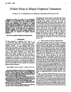
x (nm) FIG. 3. (a) The profile of the gate potential V (x) along the curved BLG. The reversed polarity at the two ends gives rise to mid-gap states, localized in x-direction. The density profile of three right-moving states, whose energy E is inside the gap ∆g , allows us to estimate the localization lengths ξ: (b) V0 = 100 meV, E = 29.13 meV, d = R (dashed white line in Fig. 2), ξ ≈ 9 and 8 nm, and (c) V0 = 10 meV, E = 3.49 meV, d = R, ξ ≈ 30 and 24 nm. We note that states with larger momenta have shorter localization lengths. (d) The √ localization length follows approximately ξ˜ = ξ −ξ0 ∝ 1/ V0 . The circles are extracted from our numerical calculations, ξ = hx2 i, for energies in the middle of the gap ∆g , equivalent to the white dashed line in Fig. 2. The lines are fits, ξ˜ ∝ 1/V0p , for the states at large kz (p = 0.59), shown as dashed lines, and for the states near kz = 0 (p = 0.52), shown as full lines.

(4)

see Fig. 2, which also contains numerical estimates for realistic parameters. We note that ∆g is enhanced by electron-electron interactions [26], however, we neglect this supportive effect herein. If the chemical √ potential is tuned inside the gap 2∆g [µ ≈ (V0 /2 2) ± β], there are three right- and three left-propagating modes. Four states at finite momentum (two left-moving and two right-moving states) are only slightly affected by the magnetic field and thus can still be considered to carry opposite spins, meaning that the total spin transfer is close to zero and these modes are not contributing to spin-filtering. In contrast to that, the two modes with kz ≈ 0 are helical modes: they have opposite velocities and opposite spins. Thus, similar to Rashba nanowires [18], the BLG quantum wire can be used as a spin filter device. Moreover, if the BLG is brought into proximity to an swave superconductor, the states with opposite momenta

and spins get paired. Working in the linearized model of left-right movers [27], we obtain the effective Bogoliubovde Gennes Hamiltonian for each of the three pairs, j = 1, 2, 3, written in Nambu space, Hsj = ~υj kj χ3 + ∆s ω2 χ2 ,

(5)

where υj is the velocity for the jth pair at the Fermi level and ∆s is the strength of the proximity-induced superconductivity, and the Pauli matrices χi (ωi ) act in the left-right mover (electron-hole) space. We note that we are in the regime corresponding to strong SOI where we keep only the slowest decaying contributions of the wave functions [27]. To determine the potential existence of MFs in the system, one can study the topological class of Hsj [28]. This Hamiltonian belongs to the topological class BDI. However, by analogy with multiband nanowires [29], additional scattering between states would bring the system into the D class. An alterna-

4 tive way of classification, which determines explicitly the number of MF bound states, is to study the null-space of the Wronskian associated with the Schr¨ odinger equation [30]. In our case, we find three MFs at each wire end in the topological phase defined by ∆2g ≥ ∆2s + δµ2 , where δµ is the chemical potential counted from the midgap level ∆g . These MFs are generically hybridized into one MF and one non-zero energy fermion by perturbations such as electron-electron interactions and interband scattering. Numerical calculation. Above we have studied the system analytically, assuming a step-like potential. In this section we compare our results with the numerical solution of the Schr¨ odinger equation for the effece 0 + Hso + Hsc + HZ , with a more tive Hamiltonian H realistic (smooth) potential, V (x) = (V0 /2) tanh(x/d), where d is the distance between the gates. The spinorbit interaction β(x) is finite only within the curved region of the BLG sheet. Along the z-direction, the system is translationally invariant, so the envelope function is given by Ψ(x, z) = eikz z ψkz (x). The profile of ψkz (x) is presented in Fig. 3. The localization length follows a power law ξ − ξ0 ∝ 1/V0p , with p ≈ 1/2, and the shift ξ0 < d is due to the finite distance between gates. In the limit d → 0, where the analytical solution is applicable, the localization length is essentially given by √ ξ = 25/4 ~υF / V0 t⊥ [15], since corrections due to SOI are of negligible higher order in β. Tunnel junction. The dependence of ξ on the potential V0 can be exploited to couple parallel wires. For instance, consider two similar quantum wires, running parallel to each other at a distance D. If ξ  D for each wire, then they are completely decoupled. However, lowering the potential in both wires locally around a point z0 on the z-axis, such that ξ0 ≈ D, we can enforce wavefunction overlap, leading to a transverse tunnel junction between the two wires at z0 . In this way, an entire network of helical wires can be envisaged. We mention that such networks could provide a platform for implementing braiding schemes for MFs [31]. Conclusions. The confinement of states in BLG into an effective quantum wire is achieved by pairs of gates with opposite polarities, leading to eight propagating modes [15]. If the direction of the wire is chosen such that the chiral angle vanishes, both valleys K and K 0 are projected onto zero momentum kz . The SOI, substantially enhanced by curvature, defines a spin quantization axis and splits spin-up and spin-down states. A magnetic field assisted by intervalley scattering opens up a gap at the center of the Brillouin zone. If the chemical potential is tuned inside the gap, three right- and three left-propagating modes emerge, so that the system possesses helical modes, which are of potential use for spinfiltering. In the proximity to an s-wave superconductor, the BLG wire hosts Majorana fermions arising from the helical modes. By locally changing the confinement po-

tential and thus the localization lengths, parallel wires can be tunnel coupled. This mechanism can be used to implement braiding of MFs in bilayer graphene. This work is supported by the Swiss NSF, NCCR Nanoscience, and NCCR QSIT.

[1] K. S. Novoselov, A. K. Geim, S. V. Morozov, D. Jiang, M. I. Katsnelson, I. V. Grigorieva, S. V. Dubonos, and A. A. Firsov, Nature (London) 438, 197 (2005). [2] A. H. Castro Neto, F. Guinea, N. M. R. Peres, K. S. Novoselov, and A. K. Geim, Rev. Mod. Phys. 81, 109 (2009). [3] R. Saito, G. Dresselhaus, and M. S. Dresselhaus, Physical Properties of Carbon Nanotubes (Imperial College Press, 1998). [4] E. McCann, arXiv:1205.4849. [5] A. K. Geim and K. S. Novoselov, Nature Materials 6, 183 (2007). [6] R. T. Weitz, M. T. Allen, B. E. Feldman, J. Martin, and A. Yacoby, Science 330, 812 (2010). [7] J. R. Williams, T. Low, M. S. Lundstrom, and C. M. Marcus, Nature Nanotechnology 6, 222 (2011). [8] M. T. Allen, J. Martin, and A. Yacoby, Nature Communications 3, 934 (2012). [9] A. S. M. Goossens, S. C. Driessen, T. A. Baart, K. Watanabe, T. Taniguchi, and L. M. Vandersypen, arXiv:1205.5825. [10] C. L. Kane and E. J. Mele, Phys. Rev. Lett. 95, 226801 (2005). [11] H. Min, J. E. Hill, N. A. Sinitsyn, B. R. Sahu, L. Kleinman, and A. H. MacDonald, Phys. Rev. B 74, 165310 (2006). [12] M. Gmitra, S. Konschuh, C. Ertler, C. Ambrosch-Draxl, and J. Fabian, Phys. Rev. B 80, 235431 (2009). [13] S. Konschuh, M. Gmitra, D. Kochan, and J. Fabian, Phys. Rev. B 85, 115423 (2012). [14] F. Mireles and J. Schliemann, arXiv:1203.1094. [15] I. Martin, Y. M. Blanter, and A. F. Morpurgo, Phys. Rev. Lett. 100, 036804 (2008). [16] Z. Qiao, J. Jung, Q. Niu, and A. H. MacDonald, Nano Letters 11, 3453 (2011). [17] M. Zarenia, J. M. Pereira, G. A. Farias, and F. M. Peeters, Phys. Rev. B 84, 125451 (2011). ˇ [18] P. Stˇreda and P. Seba, Phys. Rev. Lett. 90, 256601 (2003). [19] M. Z. Hasan and C. L. Kane, Rev. Mod. Phys. 82, 3045 (2010). [20] J. Klinovaja, M. J. Schmidt, B. Braunecker, and D. Loss, Phys. Rev. Lett. 106, 156809 (2011). [21] J. Klinovaja, S. Gangadharaiah, and D. Loss, Phys. Rev. Lett. 108, 196804 (2012). [22] J. Alicea, Rep. Prog. Phys. 75, 076501 (2012). [23] F. Kuemmeth, S. Ilani, D. C. Ralph, and P. L. McEuen, Nature 452, 448 (2008). [24] W. Izumida, K. Sato, and R. Saito, J. Phys. Soc. Jpn. 78, 074707 (2009). [25] J. Klinovaja, M. J. Schmidt, B. Braunecker, and D. Loss, Phys. Rev. B 84, 085452 (2011). [26] B. Braunecker, G. I. Japaridze, J. Klinovaja, and D. Loss, Phys. Rev. B 82, 045127 (2010).

5 [27] J. Klinovaja and D. Loss, Phys. Rev. B 86, 085408 (2012). [28] S. Ryu, A. P. Schnyder, A. Furusaki, and A. W. W. Ludwig, New Journal of Physics 12, 065010 (2010).

[29] S. Tewari and J. D. Sau, arXiv:1111.6592. [30] J. Klinovaja, P. Stano, and D. Loss, arXiv:1207.7322. [31] J. Alicea, Y. Oreg, G. Refael, F. von Oppen, and M. P. A. Fisher, Nature Physics 7, 412 (2011).