Hidden Markov Models for ILM Appliance Identification

Available online at www.sciencedirect.com

ScienceDirect Procedia Computer Science 32 (2014) 1010 – 1015

International Workshop on Enabling ICT for Smart Buildings (ICT-SB 2014)

Hidden Markov Models for ILM appliance identification Antonio Ridia,b , Jean Henneberta,b a iCoSys,

University of Applied Sciences of Western Switzerland, Boulevard de P´erolles 80, 1700 Fribourg, Switzerland b DIUF, University of Fribourg, Boulevard de P´ erolles 90, 1700 Fribourg, Switzerland

Abstract The automatic recognition of appliances through the monitoring of their electricity consumption finds many applications in smart buildings. In this paper we discuss the use of Hidden Markov Models (HMMs) for appliance recognition using so-called intrusive load monitoring (ILM) devices. Our motivation is found in the observation of electric signatures of appliances that usually show time varying profiles depending to the use made of the appliance or to the intrinsic internal operating of the appliance. To determine the benefit of such modelling, we propose a comparison of stateless modelling based on Gaussian mixture models and state-based models using Hidden Markov Models. The comparison is run on the publicly available database ACS-F1. We also compare different approaches to determine the best model topologies. More specifically we compare the use of a priori information on the device, a procedure based on a criteria of log-likelihood maximization and a heuristic approach. © 2014 Published by Elsevier B.V. Open access under CC BY-NC-ND license. c 2014 The Published by Elsevier B.V. Selection andAuthors. Peer-review under responsibility of the Program Chairs. Selection and peer-review under responsibility of Elhadi M. Shakshuki.

Keywords: Hidden Markov Model; appliance recognition; Intrusive Load Monitoring (ILM)

1. Introduction In developed countries, the electrical consumption in buildings represents a major source of the energy bill. Intelligent building management system (IBMS) can save energy using information on building physic and details about its sub-systems utilization 1 . For instance, IBMS can turn on and off appliances or change their state for optimizing energetic consumption while preserving human comfort. The electrical consumption analysis is able to provide useful information for potentially identifying appliances currently in use and their state. Appliances recognition task entails different difficulties depending on the acquisition protocol. Two approaches are used in most of the cases: Intrusive Load Monitoring (ILM) and Non-Intrusive Load Monitoring (NILM). In ILM approaches, multiple sensors are generally used and distributed in the environment. Sensors are placed at panel level, plug level or directly on a single appliance. The granularity depends on the number of aggregated appliances. In the ∗

Corresponding author. Tel.: +41-26-4296961 ; fax: +41-26-4296600. E-mail address: [email protected]

1877-0509 © 2014 Published by Elsevier B.V. Open access under CC BY-NC-ND license.

Selection and Peer-review under responsibility of the Program Chairs. doi:10.1016/j.procs.2014.05.526

Antonio Ridi and Jean Hennebert / Procedia Computer Science 32 (2014) 1010 – 1015

1011

most common case, we have one sensor per appliance. In NILM approach, on the contrary, only one smart meter is placed at the panel level. The electrical consumption of the whole habitation is aggregated in one signal. The appliance recognition is usually achieved using machine learning techniques. When appliance signatures are superposed, disaggregation algorithms for recovering each appliance contribution are effective. Disaggregation algorithms are usually applied in NILM approach, but also in ILM systems with aggregated data. When one sensor per appliance is used, the recognition task is different as signals are already separated. Many machine learning techniques have been successfully applied 2 . In this paper we focus on the use of Hidden Markov Model. Given the state-base nature of electrical appliances, their signatures are particularly suitable for state-base modeling. For instance, some appliances such as fridges or microwaves can be thought as finite-state machines. Their real states (as stand-by, compression phase, etc.) can be represented by hidden states in the Markov chain. In Section 2 we provide details about related works using HMM in the appliance identification context. In Section 3 we explain our procedure for the application of HMM. In Section 4 we present our result and discussion. We conclude the paper in Section 5.

2. Related Works Several previous works have already explored the use of HMMs and similar algorithms on NILM and ILM signatures. However, there are major differences among studies depending on the hidden states meaning and how they are applied. Durand et al. 3 analyzed the total electrical consumption of 100 houses measured for a year. The measure frequency was of one sample every ten minutes. They modelled with an hidden Markov chain the residuals from the log-consumption against the estimation of fixed factors, as the month, day, hours, type of contract and maximal power. In their paper, they interpreted the hidden states as domestic activities such as resting, washing or meal preparation. They chose a model with seven states, as the simplest model among those pre-selected using the Bayesian information criterion, integrated completed likelihood and half-sample bootstrap. They computed the state sequences and correlated the electrical appliances consumption using a contingency table. Zia et al. 4 proposed an HMM based method for differentiating individual electrical signatures from their combined profiles. In a first phase, they built an HMM for every individual load. They adapted the number of states and the topology depending on the appliance category characteristics. For instance the category fridge has been modelled using the chronological sequence of its states, derived from the repetition of the compression / non compression phases. A second phase consisted in merging the models in one HMM, where a state is a combination of the HMM of appliances. Finally, with the Viterbi algorithm, they aligned the sequence of states and recovered the appliances operational mode. Their approach has been tested on fridge, dishwasher, microwave, computer and printer. Kolter et al. 5 proposed the REDD database and used Factorial HMM (FHMM) for disaggregating the electrical signature. The FHMM can be understood as an HMM with distributed state representation coupled by observations 6 . With FHMM, each device is modelled using one HMM. In the specific case of the paper, every HMM is described by four states. Inference can be injected knowing the total consumption, that can be thought as the sum of single HMMs. Other works are also based on FHMM, as in 7,8,9,10 . Parson et al. 11 proposed a disaggregation approach on the REDD database modelling three appliances, namely refrigerator, clothes dryer and microwave and searching for them in the total consumption signal. They trained the models using the appliance signals and disaggregated the appliances in parallel. Given that the total electrical consumption includes other appliances, they proposed a modification of the Viterbi algorithm, filtering the observation where the joint probability is below a given threshold. They disaggregated the 35% of the total energy consumption with an accuracy of 85%. Kim 8 performed and compared different methods for the disaggregation based on HMM: FHMM, conditional FHMM (CFHMM), factorial hidden semi-Markov model (FHSMM), conditional FHSMM (CFHSMM). In the conditional case, additional features are injected such as time of day, dependency between appliances and sensor measurements. Semi-hidden Markov model (SHMM) are thought to improve results, because they include explicit duration and it is potentially useful for different appliances. The appliances are modeled with two states on and off. They found out that CFHSMM are leading to the best performances.

1012


Other methods derived from state-based modelling have been proposed, as modification of the Viterbi algorithm for taking into account a priori data on the appliances used 12 or Hierarchical Dirichlet Process Hidden semi-Markov Model (HDP-HSMM) for data disaggregation 13 .

3. Methods We based our experiments on the ACS-F1 database that can be found under www.watt-ict.com. The ACS-F1 database is a collection of electrical appliances signatures spread among 10 different categories 14 . Each category contains 10 appliances of different brands or models. A given appliance is recorded during 2 hours, split into 2 sessions of 1 hour. The sampling frequency is 0.1 Hz. The categories are : mobile phone, coffee machine, computer workstation with monitor, fridge and freezer, Hi-Fi system, lamp, laptop, microwave oven, printer, and television. Two evaluation protocols are provided with the database, allowing teams to compare their results. The first protocol, called intersession, uses the first hour of all appliance for training and the other hour for testing. The signals are different between the training and the test set, but they are observed from the same appliances. The second protocol, called unseen appliance, uses a 10-fold cross validation to allow testing on appliances not seen in the training set. The unseen appliance protocol is expected to be more difficult than the intersession protocol. More details about the protocols are available from 14 . Some works based on these protocols have been presented in 15,16 . An observed signature is a sequence of vectors O = {o1 , . . . , oN } where a vector on is composed of 6 coefficients: real power (W), reactive power (var), RMS current (A), RMS voltage (V), frequency (Hz) and phase of voltage relative to current (ϕ). In our experiments, an observation on is transformed into a 18 coefficients feature vector xn composed of the original observation coefficients and complemented with the delta (velocity) and delta-delta (acceleration) coefficients. Delta and delta-delta coefficients have been demonstrated to inject useful information 16 . In previous works Gaussian Mixture Model (GMM) and K-Nearest Neighbor (k-NN) algorithms have been successfully applied to the ACS-F1 database 15,16 . Such algorithms are stateless, i.e. the temporal characteristics of the time sequence and the fact that the electricity consumption may follow a sequence of modes is not used in the modelling. In this work, we are interested in the use of state-based models. Our motivation is found in the observation of electric signatures of appliances that usually show time varying profiles depending to the use made of the appliance or to the intrinsic internal operating of the appliance. A natural modelling scheme when attempting to capture a notion of states is Hidden Markov Models (HMMs). With such modelling, the learning problem can be separated into two sub-problems: determining the structure of models and learning its parameters. In HMM the structure of the model is defined by the topology and number of states, while transition and emission probabilities are two typical parameters to be learned. For completely defining an HMM the following parameters are needed: • • • •

The number of states of the model (Q) The set of state transition probabilities (A = ai j where 1..i, j..Q) The probability distribution in each of the states (B = b j (k) where 1.. j..Q, 1..k..D; D is the space dimension) The initial state distribution (π = πi where 1..i..Q)

In our experiment, we consider ergodic HMMs, i.e. topologies where a given state is connected to all other states. This choice is motivated as the use made of the different appliances is not known a priori and may show a stochastic nature according to the user. For example, there is a priori no knowledge of the sequence of change of power of a microwave, which is bound to the needs of the user. In the case of ergodic HMMs, the only parameter of the structure is the number of states. Different strategies can be used to determine the best number of states per models. A straightforward strategy is to rely on heuristic strategies. It consists in computing all the possible combinations and select the one that performs the best. Other more complex strategies consists in starting with a certain number of states and varying their number with bottom-up or top down approaches. In top-down approaches, models are evaluated by starting with a large number of states and successively merging them, as in Bayesian model merging 17 . In bottomup approaches, models are generated starting from few states (at least one) and splitting them in new states, as in Maximum-likelihood successive-state-splitting 18 19 . Details about splitting or merging algorithms depend on specific criterion rules. Models have to be compared for choosing the winner. Many criterion exist, as Akaike information criterion, Bayesian information criterion, integrated completed likelihood 3 .

1013


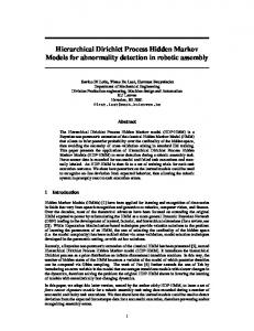
a)

b)

c)

d)

Fig. 1. Ergodic models with respectively 1, 2, 3 and 4 states. The number of Gaussians per model is kept constant for controlled experiments.

In this paper we propose to use two methods: the log-likelihood-maximization and a heuristic methods. With the first method, we start with one state and we increment iteratively the number of states. The selected topology is the one leading to the highest log-likelihood on the training set. The second method consists in computing all the possible combinations and choosing the one a posteriori leading to the higher accuracy rate. In both cases we compute four different ergodic models: one-state (equivalent to GMM), two-states, three-states and four-states models. We also constrain ourselves to perform controlled experiments, i.e. using the same number of model parameters from one topology to the other. We therefore chose to use 12 Gaussians because this value is the least common multiple among the possible number of states for topologies from 1 to 4 states. Moreover, previous works have shown that 12 Gaussians is a good compromise between accuracy rate and computational complexity 15 . The Gaussians are spread uniformly among states. As a consequence, the one-state model contains 12 Gaussians, the two-state model has 6 Gaussians per state, the three-state model has 4 Gaussians per state and the four-state model has 3 Gaussians per state. These different topologies are illustrated in Fig. 1.

4. Result and discussion In Table I, we report the best number of states found using the different approaches and protocols for all categories. HMML and HMMH refers to the log-likelihood maximization and heuristic methods respectively. The intersession protocol is abbreviated as P1 and the unseen appliance protocol is abbreviated as P2. Table 1. Number of states in the best configurations using the log-likelihood maximization (HMML ) and heuristic (HMMH ) methods on the intersession (P1) and unseen appliance (P2) protocols Category

HMML P1

HMMH P1

HMML P2

HMMH P2

hifi television mobile phone coffee machine computer-monitor fridge-freezer lamp laptop microwave printer

3 3 4 4 4 3 4 3 3 3

1 1 1 1 4 1 1 4 1 1

4 4 4 4 3 4 4 4 4 4

2 1 2 1 2 3 3 3 4 3

1014


The number of states varies between experiments. Using HMML , the configurations with 3 or 4 states are maximizing the maximum likelihood criterion for each category. Using HMMH different results are obtained depending on the protocol. Protocol P1 is easier and per nature shows less variability between the training and testing sets. Simple modelling with single state models (actually GMMs) reveals robust enough. Protocol P2, on the other side, has a larger variability and the heuristic approach shows the benefit of using more complex models capturing state dependence. Table 2. Accuracy rate using GMM and HMM with log-likelihood maximization and heuristic methods on the intersession and unseen appliance protocols Category

GMM P1

HMML P1

HMMH P1

GMM P2

HMML P2

HMMH P2

hifi television mobile phone coffee machine computer-monitor fridge-freezer lamp laptop microwave printer Mean

1 1 1 1 .6 1 .9 .8 1 .8 .91

.9 .9 .8 1 .9 1 .8 .7 1 .9 .89

1 1 1 1 .8 1 .9 .8 1 .8 .93

.5 .4 .95 .8 .6 .85 .45 .6 .75 .7 .66

.55 .4 .8 .8 .55 .95 .55 .4 .85 .65 .65

.6 .45 .9 .85 .7 1 .6 .65 .9 .7 .74

In Table 2, we report the accuracy rate using the selected configurations. We also compared the results using a 12 Gaussians GMM. We observe that the configurations based on HMML perform slightly worse than GMM. Using protocol P1, the accuracy decreases from 91% to 89%, while in the second it goes from 66% to 65%. Attempting to find the best topology using the log-likelihood method do not seem to be reliable in the case of this data set. The reason is probably to be found in the relatively small quantity of data and potential overfitting as the max loglikelihood is computed on the training set. We also observe that some categories such as computer-monitor, coffee machine, microwave, fridge-freezer reach equal or better accuracy with the HMML configurations. We observe that the HMMH configurations perform better than GMM for both protocols, with an increase from 91% to 93% for P1 and from 66% to 74% for P2. Systematic improvement for most categories are observed.

5. Conclusion In this paper we discussed the use of HMMs for the task of ILM appliance identification. The evaluation is carried on using the ACS-F1 database, containing electrical appliance signatures recorded at low sampling frequency spread among 10 categories. We evaluated the results using the two protocols P1 and P2 provided with the database. In a first step, we searched for the best HMM structures for each category. We used two approaches: maximum log-likelihood (HMML ) and heuristic (HMMH ). In order to perform controlled and comparable evaluations, we maintained the complexity constant between models, i.e. imposing a fixed number of parameters through all models. In the second phase we used the best HMM configurations and we computed the accuracy rates for each category. Finally we compared the results of the HMM configurations with a baseline GMM algorithm for both protocols. Interestingly, the GMM performed better than the HMML configuration. The maximum log-likelihood criterion seems not suitable on this database and a phenomenon of over-fitting is suspected considering the relatively small size of the database. On the other side, the HMMH configurations outperformed significantly the GMM, especially for the most difficult and realistic protocol P2. Imposing fixed parameters through all models, as the total number of Gaussians, can lead to a suboptimal solution. This choice is a compromise between accuracy rate and computational complexity. In future works we intend to use different approaches, consisting in increasing the learning algorithm capacity for finding the best solution. Finally, for generalizing our statements about the algorithms comparison, we intend to perform a statistical evaluation of classifiers.


1015

6. Acknowledgment This work was supported by the research grant of the Hasler Foundation project Green-Mod, by the HES-SO and by the University of Fribourg in Switzerland.

References 1. Agarwal, Y., Balaji, B., Gupta, R., Lyles, J., Wei, M., Weng, T.. Occupancy-driven energy management for smart building automation. In: Proceedings of the 2nd ACM Workshop on Embedded Sensing Systems for Energy-Efficiency in Building. 2010, p. 1–6. 2. Ridi, A., Gisler, C., Hennebert, J.. A survey on intrusive load monitoring for appliance recognition. In: Proceedings of the 22nd International Conference on Pattern Recognition, to appear. 2014, . 3. Durand, J.B., Bozzi, L., Celeux, G., Derquenne, C.. Analyse de courbes de consommation electrique par chaines de markov cachees. Revue de statistique appliquee 2004;52(4):71–91. 4. Zia, T., Bruckner, D., Zaidi, A.. A Hidden Markov Model Based Procedure for Identifying Household Electric Loads. In: IECON 2011 37th Annual Conference on IEEE Industrial Electronics Society. 2011, p. 3218–3223. 5. Kolter, J.Z., Johnson, M.J.. REDD : A Public Data Set for Energy Disaggregation Research. In: Proceedings of the ACM Workshop on Data Mining Applications in Sustainability. 2011, . 6. Ghahramani, Z., Jordan, M.I.. Factorial hidden markov models. Machine Learning 1997;29(2–3):245–273. 7. Robert, L., Liszewski, K.. Methods of Electrical Appliances Identification in Systems Monitoring Electrical Energy Consumption. In: The 7th IEEE International Conference on Intelligent Data Acquisition and Advanced Computing Systems: Technology and Applications. 2013, p. 10–14. 8. Kim, H.S.. Unsupervised disaggregation of low frequency power measurement. Ph.D. thesis; University of Illinois at Urbana-Champaign; 2012. 9. Akshay Uttama Nambi, S.N., Papaioannou, T.G., Chakraborty, D., Aberer, K.. Sustainable energy consumption monitoring in residential settings. 2013 IEEE Conference on Computer Communications Workshops 2013;. 10. Zoha, A., Gluhak, A., Nati, M., Imran, M.A.. Low-power appliance monitoring using Factorial Hidden Markov Models. 2013 IEEE 8th International Conference on Intelligent Sensors, Sensor Networks and Information Processing 2013;12:527–532. 11. Parson, O., Ghosh, S., Weal, M., Rogers, A.. Using hidden markov models for iterative non-intrusive appliance monitoring. In: Neural Information Processing Systems, Workshop on Machine Learning for Sustainability. 2011, . 12. Zeifman, M., Roth, K.. Viterbi algorithm with sparse transitions (VAST) for nonintrusive load monitoring. In: 2011 IEEE Symposium on Computational Intelligence Applications In Smart Grid (CIASG). 2011, p. 1–8. 13. Johnson, M.J., Willsky, A.S.. Bayesian nonparametric hidden semi-markov models. Tech. Rep.; Massachusetts Institute of Technology; 2012. 14. Gisler, C., Ridi, A., Zufferey, D., Khaled, O.A., Hennebert, J.. Appliance consumption signature database and recognition test protocols. In: Proceedings of the 8th International Workshop on Systems, Signal Processing and their Applications (Wosspa ’13). 2013, p. 336–341. 15. Ridi, A., Gisler, C., Hennebert, J.. Automatic identification of electrical appliances using smart plugs. In: Proceedings of the 8th International Workshop on Systems, Signal Processing and their Applications (Wosspa ’13). 2013, p. 301–305. 16. Ridi, A., Gisler, C., Hennebert, J.. Unseen appliances identification. In: Proceedings of the 18th Iberoamerican Congress on Pattern Recognition (Ciarp ’13). 2013, p. 75–82. 17. Stolcke, A., Omohundro, S.. Hidden Markov Model Induction by Bayesian Model Merging. In: Advances in Neural Information Processing Systems. 1993, p. 11–18. 18. Singer, H., Oskndorf, M.. Maximum likelihood successive state splitting. In: Proceedings of the IEEE, ICASSP-96; vol. 2. 1996, p. 601–604. 19. Li, C., Biswas, G.. Temporal pattern generation using hidden markov model based unsupervised classification. Advances in Intelligent data analysis 1999;1642.