High Performance Numerical Computing for High Energy Physics: A ...

Hindawi Publishing Corporation Advances in High Energy Physics Volume 2014, Article ID 507690, 13 pages http://dx.doi.org/10.1155/2014/507690

Research Article High Performance Numerical Computing for High Energy Physics: A New Challenge for Big Data Science Florin Pop Computer Science Department, Faculty of Automatic Control and Computers, University Politehnica of Bucharest, Splaiul Independentei 313, Bucharest 060042, Romania Correspondence should be addressed to Florin Pop; [email protected] Received 20 September 2013; Revised 23 December 2013; Accepted 26 December 2013 Academic Editor: Carlo Cattani Copyright © 2014 Florin Pop. This is an open access article distributed under the Creative Commons Attribution License, which permits unrestricted use, distribution, and reproduction in any medium, provided the original work is properly cited. The publication of this article was funded by SCOAP3 . Modern physics is based on both theoretical analysis and experimental validation. Complex scenarios like subatomic dimensions, high energy, and lower absolute temperature are frontiers for many theoretical models. Simulation with stable numerical methods represents an excellent instrument for high accuracy analysis, experimental validation, and visualization. High performance computing support offers possibility to make simulations at large scale, in parallel, but the volume of data generated by these experiments creates a new challenge for Big Data Science. This paper presents existing computational methods for high energy physics (HEP) analyzed from two perspectives: numerical methods and high performance computing. The computational methods presented are Monte Carlo methods and simulations of HEP processes, Markovian Monte Carlo, unfolding methods in particle physics, kernel estimation in HEP, and Random Matrix Theory used in analysis of particles spectrum. All of these methods produce data-intensive applications, which introduce new challenges and requirements for ICT systems architecture, programming paradigms, and storage capabilities.

1. Introduction High Energy Physics (HEP) experiments are probably the main consumers of High Performance Computing (HPC) in the area of e-Science, considering numerical methods in real experiments and assisted analysis using complex simulation. Starting with quarks discovery in the last century to Higgs Boson in 2012 [1], all HEP experiments were modeled using numerical algorithms: numerical integration, interpolation, random number generation, eigenvalues computation, and so forth. Data collection from HEP experiments generates a huge volume, with a high velocity, variety, and variability and passes the common upper bounds to be considered Big Data. The numerical experiments using HPC for HEP represent a new challenge for Big Data Science. Theoretical research in HEP is related to matter (fundamental particles and Standard Model) and Universe formation basic knowledge. Beyond this, the practical research in HEP has led to the development of new analysis tools (synchrotron radiation, medical imaging or hybrid models [2],

wavelets-computational aspects [3]), new processes (cancer therapy [4], food preservation, or nuclear waste treatment), or even the birth of a new industry (Internet) [5]. This paper analyzes two aspects: the computational methods used in HEP (Monte Carlo methods and simulations, Markovian Monte Carlo, unfolding methods in particle physics, kernel estimation, and Random Matrix Theory) and the challenges and requirements for ICT systems to deal with processing of Big Data generated by HEP experiments and simulations. The motivation of using numerical methods in HEP simulations is based on special problems which can be formulated using integral or differential-integral equations (or systems of such equations), like quantum chromodynamics evolution of parton distributions inside a proton which can be described by the Gribov-Lipatov-Altarelli-Parisi (GLAP) equations [6], estimation of cross section for a typical HEP interaction (numerical integration problem), and data representation using histograms (numerical interpolation problem). Numerical methods used for solving differential

2

Advances in High Energy Physics Comparison and correction Physics model → simulation process → event generator → vectors of events

Simulated detectors

Events

Reconstruction Nature (physical experiments)

Real detectors

Vector of events

Events

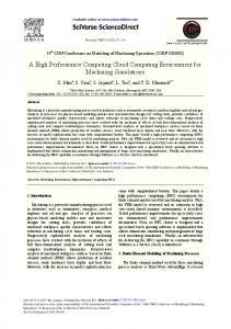
Figure 1: General approach of event generation, detection, and reconstruction.

equations or integrals are based on classical quadratures and Monte Carlo (MC) techniques. These allow generating events in terms of particle flavors and four-momenta, which is particularly useful for experimental applications. For example, MC techniques for solving the GLAP equations are based on simulated Markov chains (random walks), which have the advantage of filtering and smoothing the state vector for estimating parameters. In practice, several MC event generators and simulation tools are used. For example, HERWIG (http://projects .hepforge.org/herwig/) project considers angular-ordered parton shower, cluster hadronization (the tool is implemented using Fortran), PYTHIA (http://www.thep.lu.se/ torbjorn/Pythia.html) project is oriented on dipoletype parton shower and string hadronization (the tool is implemented in Fortran and C++), and SHERPA (http://projects.hepforge.org/sherpa/) considers dipole-type parton shower and cluster hadronization (the tool is implemented in C++). An important tool for MC simulations is GATE (GEANT4 Application for Tomographic Emission), a generic simulation platform based on GEANT4. GATE provides new features for nuclear imaging applications and includes specific modules that have been developed to meet specific requirements encountered in SPECT (Single Photon Emission Tomography) and PET (Positron Emission Tomography). The main contributions of this paper are as follows: (i) introduction and analysis of most important modeling methods used in High Energy Physics; (ii) identifying and describing of the computational numerical methods for High Energy Physics; (iii) presentation of the main challenges for Big Data processing. The paper is structured as follows. Section 2 introduces the computational methods used in HEP and describes the performance evaluation of parallel numerical algorithms. Section 3 discusses the new challenge for Big Data Science generated by HEP and HPC. Section 4 presents the conclusions and general open issues.

2. Computational Methods Used in High Energy Physics Computational methods are used in HEP in parallel with physical experiments to generate particle interactions that

are modeled using vector of events. This section presents general approach of event generation, simulation methods based on Monte Carlo algorithms, Markovian Monte Carlo chains, methods that describe unfolding processes in particle physics, Random Matrix Theory as support for particle spectrum, and kernel estimation that produce continuous estimates of the parent distribution from the empirical probability density function. The section ends with performance analysis of parallel numerical algorithms used in HEP. 2.1. General Approach of Event Generation. The most important aspect in simulation for HEP experiments is event generation. This process can be split into multiple steps, according to physical models. For example, structure of LHC (Large Hadron Collider) events: (1) hard process; (2) parton shower; (3) hadronization; (4) underlying event. According to official LHC website (http://home.web.cern.ch/about/computing): “approximately 600 million times per second, particles collide within the LHC. . .Experiments at CERN generate colossal amounts of data. The Data Centre stores it, and sends it around the world for analysis.” The analysis must produce valuable data and the simulation results must be correlated with physical experiments. Figure 1 presents the general approach of event generation, detection, and reconstruction. The physical model is used to create simulation process that produces different type of events, clustered in vector of events (e.g., the fourth type of events in LHC experiments). In parallel, the real experiments are performed. The detectors identify the most relevant events and, based on reconstruction techniques, vector of events is created. The detectors can be real or simulated (software tools) and the reconstruction phase combines real events with events detected in simulation. At the end, the final result is compared with the simulation model (especially with generated vectors of events). The model can be corrected for further experiments. The goal is to obtain high accuracy and precision of measured and processed data. Software tools for event generation are based on random number generators. There are three types of random numbers: truly random numbers (from physical generators), pseudorandom numbers (from mathematical generators), and quasirandom numbers (special correlated sequences of numbers, used only for integration). For example, numerical integration using quasirandom numbers usually gives faster convergence than the standard integration methods based on

Advances in High Energy Physics

3

(1) procedure Random Generator Poisson(𝜇) (2) 𝑛𝑢𝑚𝑏𝑒𝑟 ← −1; (3) 𝑎𝑐𝑐𝑢𝑚𝑢𝑙𝑎𝑡𝑜𝑟 ← 1.0; (4) 𝑞 ← exp {−𝜇}; (5) while 𝑎𝑐𝑐𝑢𝑚𝑢𝑙𝑎𝑡𝑜𝑟 > 𝑞 do (6) 𝑟𝑛𝑑 𝑛𝑢𝑚𝑏𝑒𝑟 ← 𝑅𝑁𝐷() ; (7) 𝑎𝑐𝑐𝑢𝑚𝑢𝑙𝑎𝑡𝑜𝑟 ← 𝑎𝑐𝑐𝑢𝑚𝑢𝑙𝑎𝑡𝑜𝑟 ∗ 𝑟𝑛𝑑 𝑛𝑢𝑚𝑏𝑒𝑟; (8) 𝑛𝑢𝑚𝑏𝑒𝑟 ← 𝑛𝑢𝑚𝑏𝑒𝑟 + 1; (9) end while (10) return number; (11) end procedure Algorithm 1: Random number generation for Poisson distribution using many random generated numbers with normal distribution (RND).

𝑃 [𝑋 = 𝑘] =

𝜇𝑘 exp {−𝜇} , 𝑘!

𝑘 = 0, 1, . . . ,

Random generator Poisson (Alg. 1) Frequency

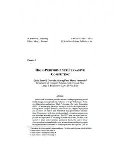
quadratures. In event generation pseudorandom numbers are used most often. The most popular HEP application uses Poisson distribution combined with a basic normal distribution. The Poisson distribution can be formulated as

350000 300000 250000 200000 150000 100000 50000 0 0

(1)

5

10 15 20 Generted numbers

25

30

(a)

Frequency

with 𝐸(𝑘) = 𝑉(𝑘) = 𝜇 (𝑉 is variance and 𝐸 is expectation value). Having a uniform random number generator called RND() (Random based on Normal Distribution) we can use the following two algorithms for event generation techniques. The result of running Algorithms 1 and 2 to generate around 106 random numbers is presented in Figure 2. In general, the second algorithm has better result for Poisson distribution. General recommendation for HEP experiments indicates the use of popular random number generators like TRNG (True Random Number Generators), RANMAR (Fast Uniform Random Number Generator used in CERN experiments), RANLUX (algorithm developed by Luscher used by Unix random number generators), and Mersenne Twister (the “industry standard”). Random number generators provided with compilers, operating system, and programming language libraries can have serious problem because they are based on system clock and suffer from lack of uniformity of distribution for large amounts of generated numbers and correlation of successive values. The art of event generation is to use appropriate combinations of various random number generation methods in order to construct an efficient event generation algorithm being solution to a given problem in HEP.

Random generator Poisson RND (Alg. 2) 400000 350000 300000 250000 200000 150000 100000 50000 0 0

5

10 15 20 Generted numbers

25

(b)

Figure 2: General approach of event generation, detection, and reconstruction.

advance. If 𝜌(𝑟) is the probability density function, 𝜌(𝑟)𝑑𝑟 = 𝑃[𝑟 < 𝑟󸀠 < 𝑟 + 𝑑𝑟], the cumulative distributed function is 𝐶 (𝑟) = ∫

𝑟

−∞

𝜌 (𝑥) 𝑑𝑥 󳨐⇒ 𝜌 (𝑟) =

𝑑𝐶 (𝑟) . 𝑑𝑟

(2)

𝐶(𝑟) is a monotonically nondecreasing function with all values in [0, 1]. The expectation value is 𝐸 (𝑓) = ∫ 𝑓 (𝑟) 𝑑𝐶 (𝑟) = ∫ 𝑓 (𝑟) 𝜌 (𝑟) 𝑑𝑟.

2.2. Monte Carlo Simulation and Markovian Monte Carlo Chains in HEP. In general, a Monte Carlo (MC) method is any simulation technique that uses random numbers to solve a well-defined problem, 𝑃. If 𝐹 is a solution of the problem ̂ an 𝑃 (e.g., 𝐹 ∈ 𝑅𝑛 or 𝐹 has a Boolean value), we define 𝐹, ̂ estimation of 𝐹, as 𝐹 = 𝑓({𝑟1 , 𝑟2 , . . . , 𝑟𝑛 }, . . .), where {𝑟𝑖 }1≤𝑖≤𝑛 is a random variable that can take more than one value and for which any value that will be taken cannot be predicted in

30

(3)

And the variance is 2

𝑉 (𝑓) = 𝐸[𝑓 − 𝐸 (𝑓)] = 𝐸 (𝑓2 ) − 𝐸2 (𝑓) .

(4)

2.2.1. Monte Carlo Event Generation and Simulation. To define a MC estimator the “Law of Large Numbers (LLN)” is used. LLN can be described as follows: let one choose 𝑛

4


(1) procedure Random Generator Poisson RND(𝜇, 𝑟) (2) 𝑛𝑢𝑚𝑏𝑒𝑟 ← 0; (3) 𝑞 ← exp {−𝜇}; (4) 𝑎𝑐𝑐𝑢𝑚𝑢𝑙𝑎𝑡𝑜𝑟 ← 𝑞; (5) 𝑝 ← 𝑞; (6) while 𝑟 > 𝑎𝑐𝑐𝑢𝑚𝑢𝑙𝑎𝑡𝑜𝑟 do (7) 𝑛𝑢𝑚𝑏𝑒𝑟 ← 𝑛𝑢𝑚𝑏𝑒𝑟 + 1; (8) 𝑝 ← 𝑝 ∗ 𝜇/𝑛𝑢𝑚𝑏𝑒𝑟; (9) 𝑎𝑐𝑐𝑢𝑚𝑢𝑙𝑎𝑡𝑜𝑟 ← 𝑎𝑐𝑐𝑢𝑚𝑢𝑙𝑎𝑡𝑜𝑟 + 𝑝; (10) end while (11) return number; (12) end procedure Algorithm 2: Random number generation for Poisson distribution using one random generated number with normal distribution.

numbers 𝑟𝑖 randomly, with the probability density function uniform on a specific interval (𝑎, 𝑏), each 𝑟𝑖 being used to evaluate 𝑓(𝑟𝑖 ). For large 𝑛 (consistent estimator), 𝑏 1 𝑛 1 ∑𝑓 (𝑟𝑖 ) 󳨀→ 𝐸 (𝑓) = ∫ 𝑓 (𝑟) 𝑑𝑟. 𝑛 𝑖=1 𝑏−𝑎 𝑎

(5)

The properties of a MC estimator are being normally distributed (with Gaussian density); the standard deviation is 𝜎 = √𝑉(𝑓)/𝑛; MC is unbiased for all 𝑛 (the expectation value is the real value of the integral); the estimator is consistent if 𝑉(𝑓) < ∞ (the estimator converges to the true value of the integral for every large 𝑛); a sampling phase can be applied to compute the estimator if we do not know anything about the function 𝑓; it is just suitable for integration. The sampling phase can be expressed, in a stratified way, as 𝑏

𝑟1

𝑟2

𝑏

𝑎

𝑎

𝑟1

𝑟𝑛

∫ 𝑓 (𝑟) 𝑑𝑟 = ∫ 𝑓 (𝑟) 𝑑𝑟 + ∫ 𝑓 (𝑟) 𝑑𝑟 + ⋅ ⋅ ⋅ + ∫ 𝑓 (𝑟) 𝑑𝑟. (6) MC estimations and MC event generators are necessary tools in most of HEP experiments being used at all their steps: experiments preparation, simulation running, and data analysis. An example of MC estimation is the Lorentz invariant phase space (LIPS) that describes the cross section for a typical HEP process with 𝑛 particle in the final state. Consider 𝜎𝑛 ∼ ∫ |𝑀|2 𝑑𝑅𝑛 ,

(7)

where 𝑀 is the matrix describing the interaction between particles and 𝑑𝑅𝑛 is the element of LIPS. We have the following estimation: 𝑅𝑛 (𝑃, 𝑝1 , 𝑝2 , . . . , 𝑝𝑛 ) 𝑛

𝑛

𝑘=1

𝑘=1

= ∫ 𝛿(4) (𝑃 − ∑ 𝑝𝑘 ) ∏ (𝛿 (𝑝𝑘2 − 𝑚𝑘2 ) Θ (𝑝𝑘0 ) 𝑑4 𝑝𝑘 ) , (8)

𝜇+ (q 1 )

𝜃

e+ (p1 )

𝜇− (q 2 )

e− (p2 ) z

Φ

Figure 3: Example of particle interaction: 𝑒(𝑝1 ) + 𝑒− (𝑝2 ) 𝜇+ (𝑞1 )𝜇− (𝑞2 ).

→

where 𝑃 is total four-momentum of the 𝑛-particle system; 𝑝𝑘 and 𝑚𝑘 are four-momenta and mass of the final state particles; 𝛿(4) (𝑃−∑𝑛𝑘=1 𝑝𝑘 ) is the total energy momentum conservation; 𝛿(𝑝𝑘2 − 𝑚𝑘2 ) is the on-mass-shell condition for the final state system. Based on the integration formula ∫ 𝛿 (𝑝𝑘2 − 𝑚𝑘2 ) Θ (𝑝𝑘0 ) 𝑑4 𝑝𝑘 =

𝑑3 𝑝𝑘 , 2𝑝𝑘0

(9)

obtain the iterative form for cross section: 𝑅𝑛 (𝑃, 𝑝1 , 𝑝2 , . . . , 𝑝𝑛 ) = ∫ 𝑅𝑛−1 (𝑃 − 𝑝𝑛 , 𝑝1 , 𝑝2 , . . . , 𝑝𝑛−1 )

𝑑3 𝑝𝑛 , 2𝑝𝑛0

(10)

which can be numerical integrated by using the recurrence relation. As result, we can construct a general MC algorithm for particle collision processes. Example 1. Let us consider the interaction: 𝑒+ 𝑒− → 𝜇+ 𝜇− where Higgs boson contribution is numerically negligible. Figure 3 describes this interaction (Φ is the azimuthal angle, 𝜃 the polar angle, and 𝑝1 , 𝑝2 , 𝑞1 , 𝑞2 are the four-momenta for particles). The cross section is 𝑑𝜎 =

𝛼2 [𝑊1 (𝑠) (1 + cos2 𝜃) + 𝑊2 (𝑠) cos 𝜃] 𝑑Ω, 4𝑠

(11)


5

where 𝑑Ω = 𝑑 cos 𝜃𝑑Φ, 𝛼 = 𝑒2 /4𝜋 (fine structure constant), 2 𝑠 = (𝑝10 + 𝑝20 ) is the center of mass energy squared, and 𝑊1 (𝑠) and 𝑊2 (𝑠) are constant functions. For pure processes we have 𝑊1 (𝑠) = 1 and 𝑊2 (𝑠) = 0, and the total cross section becomes 2𝜋

1

0

−1

𝜎 = ∫ 𝑑Φ ∫ 𝑑 cos 𝜃

𝑑2 𝜎 . 𝑑Φ𝑑 cos 𝜃

(12)

We introduce the following notation: 𝜌 (cos 𝜃, Φ) =

be provided in terms of Monte Carlo event generators, which directly simulate these processes and can provide unweighted (weight = 1) events. A good Monte Carlo algorithm should be used not only for numerical integration [7] (i.e., provide weighted events) but also for efficient generation of unweighted events, which is very important issue for HEP.

𝑑2 𝜎 , 𝑑Φ𝑑 cos 𝜃

(13)

̃ and let us consider 𝜌(cos 𝜃, Φ) an approximation of ̃ Now, we can compute 𝜌(cos 𝜃, Φ). Then 𝜎̃ = ∬ 𝑑Φ𝑑 cos 𝜃𝜌.

2.2.2. Markovian Monte-Carlo Chains. A classical Monte Carlo method estimates a function 𝐹 with 𝐹̂ by using a random variable. The main problem with this approach is that we cannot predict any value in advance for a random variable. In HEP simulation experiments the systems are described in states [8]. Let us consider a system with a finite set of possible states 𝑆1 , 𝑆2 , . . ., and 𝑆𝑡 the state at the moment 𝑡. The conditional probability is defined as

2𝜋

1

𝑃 (𝑆𝑡 = 𝑆𝑗 | 𝑆𝑡1 = 𝑆𝑖1 , 𝑆𝑡2 = 𝑆𝑖2 , . . . , 𝑆𝑡𝑛 = 𝑆𝑖𝑛 ) ,

0

−1

where the mappings (𝑡1 , 𝑖1 ), . . . ,(𝑡𝑛 , 𝑖𝑛 ) can be interpreted as the description of system evolution in time by specifying a specific state for each moment of time. The system is a Markov chain if the distribution of 𝑆𝑡 depends only on immediate predecessor 𝑆𝑡−1 and it is independent of all previous states as follows:

𝜎 = ∫ 𝑑Φ ∫ 𝑑 cos 𝜃𝜌 (cos 𝜃, Φ) 2𝜋

1

0

−1

= ∫ 𝑑Φ ∫ 𝑑 cos 𝜃𝑤 (cos 𝜃, Φ) 𝜌̃ (cos 𝜃, Φ) 2𝜋

1

0

−1

(14)

≈ ⟨𝑤⟩𝜌̃ ∫ 𝑑Φ ∫ 𝑑 cos 𝜃𝜌̃ (cos 𝜃, Φ) = 𝜎̃⟨𝑤⟩𝜌̃, ̃ where 𝑤(cos 𝜃, Φ) = 𝜌(cos 𝜃, Φ)/𝜌(cos 𝜃, Φ) and ⟨𝑤⟩𝜌̃ is the ̃ Here, the MC estimator is estimation of 𝑤 based on 𝜌. ⟨𝑤⟩MC =

= 𝑃 (𝑆𝑡 = 𝑆𝑗 | 𝑆𝑡−1 = 𝑆𝑖𝑡−1 ) .

1 𝑛 ∑𝑤 , 𝑛 𝑖=1 𝑖

(15)

and the standard deviation is 𝑠MC

𝑛 1 2 =( ∑(𝑤𝑖 − ⟨𝑤⟩MC ) ) 𝑛(𝑛 − 1) 𝑖=1

1/2

.

(16)

The final numerical result based on MC estimator is 𝜎MC = 𝜎̃⟨𝑤⟩MC ± 𝜎̃𝑠MC .

𝑃 (𝑆𝑡 = 𝑆𝑗 | 𝑆𝑡−1 = 𝑆𝑖𝑡−1 , . . . , 𝑆𝑡2 = 𝑆𝑖2 , 𝑆𝑡1 = 𝑆𝑖1 )

(17)

As we can show, the principle of a Monte Carlo estimator in physics is to simulate the cross section in interaction and radiation transport knowing the probability distributions (or an approximation) governing each interaction of elementary particles. Based on this result, the Monte Carlo algorithm used to ̃ generate events is as follows. It takes as input 𝜌(cos 𝜃, Φ) and in a main loop considers the following steps: (1) geñ (2) compute four-momenta erate (cos 𝜃, Φ) peer from 𝜌; ̃ The loop can be stopped 𝑝1 , 𝑝2 , 𝑞1 , 𝑞2 ; (3) compute 𝑤 = 𝜌/𝜌. in the case of unweighted events, and we will stay in the loop for weighted events. As output, the algorithm returns fourmomenta for particle for weighted events and four-momenta and an array of weights for unweighted events. The main issue is how to initialize the input of the algorithm. Based on 𝑑𝜎 formula (for 𝑊1 (𝑠) = 1 and 𝑊2 (𝑠) = 0), we can consider as ̃ input 𝜌(cos 𝜃, Φ) = (𝛼2 /4𝑠)(1 + cos2 𝜃). Then 𝜎̃ = 4𝜋𝛼2 /3𝑠. In HEP theoretical predictions used for particle collision processes modeling (as shown in presented example) should

(18)

(19)

To generate the time steps (𝑡1 , 𝑡2 , . . . , 𝑡𝑛 ) we use the probability of a single forward Markovian step given by 𝑝(𝑡 | ∞ 𝑡𝑛 ) with the property ∫𝑡 𝑝(𝑡 | 𝑡𝑛 )𝑑𝑡 = 1 and we define 𝑛 𝑝(𝑡) = 𝑝(𝑡 | 0). The 1-dimensional Monte Carlo Markovian Algorithm used to generate the time steps is presented in Algorithm 3. The main result of Algorithm 3 is that 𝑃(𝑡max ) follows a Poisson distribution: 𝑃𝑁 = ∫

𝑡max

0

𝑡max

𝑝 (𝑡1 | 𝑡0 ) 𝑑𝑡1 × ∫

𝑡1

𝑡max

× ⋅⋅⋅ × ∫

𝑡𝑁−1

×∫

∞

𝑡max

𝑝 (𝑡2 | 𝑡1 ) 𝑑𝑡2

𝑝 (𝑡𝑁 | 𝑡𝑁−1 ) 𝑑𝑡𝑁

𝑝 (𝑡𝑁+1 | 𝑡𝑁) 𝑑𝑡𝑁+1 =

(20)

1 𝑁 (𝑡 ) 𝑒−𝑡max . 𝑁! max

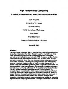
We can consider the 1-dimensional Monte Carlo Markovian Algorithm as a method used to iteratively generate the systems’ states (codified as a Markov chain) in simulation experiments. According to the Ergodic Theorem for Markov chains, the chain defined has a unique stationary probability distribution [9, 10]. Figures 4 and 5 present the running of Algorithm 3. According to different values of parameter 𝑠 used to generate the next step, the results are very different, for 1000 iterations. Figure 4 for 𝑠 = 1 shows a profile of the type of noise. For 𝑠 = 10, 100, 1000 profile looks like some of the information is filtered and lost. The best results are obtained for 𝑠 = 0.01

6


(1) Generate 𝑡1 according with 𝑝 (𝑡1 ) = 𝑝 (𝑡1 | 𝑡0 = 0) ⊳ Generate the initial state. (2) if 𝑡1 < 𝑡max then 𝑡max ⊳ Compute the initial probability. (3) 𝑃𝑁≥1 = ∫0 𝑝 (𝑡1 | 𝑡0 ) 𝑑𝑡1 ; (4) Retain 𝑡1 ; (5) end if ⊳ Discard all generated and computed data. (6) if 𝑡1 > 𝑡max then ∞ (7) 𝑁 = 0; 𝑃0 = ∫𝑡 𝑝 (𝑡1 | 𝑡0 ) 𝑑𝑡1 = 𝑒−𝑡max ; max (8) Delete 𝑡1 ; (9) EXIT. ⊳ The algorithm ends here. (10) end if (11) 𝑖 = 2; (12) while (1) do ⊳ Infinite loop until a successful EXIT. (13) Generate 𝑡𝑖 according with 𝑝 (𝑡𝑖 | 𝑡𝑖−1 ) ⊳ Generate a new state and new probability. (14) if 𝑡𝑖 < 𝑡max then 𝑡max (15) 𝑃𝑁≥𝑖 = ∫𝑡 𝑝 (𝑡𝑖 | 𝑡𝑖−1 ) 𝑑𝑡𝑖 ; 𝑖 (16) Retain 𝑡𝑖 ; (17) end if ⊳ Discard all generated and computed data. (18) if 𝑡𝑖 > 𝑡max then ∞ (19) 𝑁 = 𝑖 − 1; 𝑃𝑖 = ∫𝑡 𝑝 (𝑡𝑖 | 𝑡𝑖−1 ) 𝑑𝑡𝑖 ; max (20) Retain (𝑡1 , 𝑡2 , . . . , 𝑡𝑖−1 ); Delete 𝑡𝑖 ; (21) EXIT. ⊳ The algorithm ends here. (22) end if (23) 𝑖 = 𝑖 + 1; (24) end while Algorithm 3: 1-Dimensional Monte Carlo Markovian Algorithm.

and 𝑠 = 0.1 and the generated values can be easily accepted for MC simulation in HEP experiments. Figure 5 shows the acceptance rate of values generated with parameter 𝑠 used in the algorithm. And parameter values are correlated with Figure 4. Results in Figure 5 show that the acceptance rate decreases rapidly with increasing value of parameter 𝑠. The conclusion is that values must be kept small to obtain meaningful data. A correlation with the normal distribution is evident, showing that a small value for the mean square deviation provides useful results. 2.2.3. Performance of Numerical Algorithms Used in MC Simulations. Numerical methods used to compute MC estimator use numerical quadratures to approximate the value of the integral for function 𝑓 on a specific domain by a linear compilation of function values and weights {𝑤𝑖 }1≤𝑖≤𝑚 as follows: 𝑏

𝑚

𝑎

𝑖=1

∫ 𝑓 (𝑟) 𝑑𝑟 = ∑𝑤𝑖 𝑓 (𝑟𝑖 ) .

(21)

We can consider a consistent MC estimator 𝑎 a classical numerical quadrature with all 𝑤𝑖 = 1. Efficiency of integration methods for 1 dimension and for 𝑑 dimensions is presented in Table 1. We can conclude that quadrature methods are difficult to apply in many dimensions for variate integration domains (regions) and the integral is not easy to be estimated.

Table 1: Efficiency of integration methods for 1 dimension and for 𝑑 dimensions. Method Monte Carlo Trapezoidal rule

1 dimension 𝑛−1/2

𝑑 dimensions 𝑛−1/2

𝑛−2

𝑛−2/𝑑

−4

Simpson’s rule

𝑛

𝑛−4/𝑑

𝑚-points Gauss rule (𝑚 < 𝑛)

𝑛−2𝑚

𝑛−2𝑚/𝑑

As practical example, in a typical high-energy particle collision there can be many final-state particles (even hundreds). If we have 𝑛 final state particle, we face with 𝑑 = 3𝑛 − 4 dimensional phase space. As numerical example, for 𝑛 = 4 we have 𝑑 = 8 dimensions, which is very difficult approach for classical numerical quadratures. Full decomposition integration volume for one double number (10 Bytes) per volume unit is 𝑛𝑑 × 10 Bytes. For the example considered with 𝑑 = 8 and 𝑛 = 10 divisions for interval [0, 1] we have, for one numerical integration, 𝑛𝑑 × 10 Bytes =

108 × 10 𝐺 Bytes ≈ 0.93 𝐺 Bytes. 10243

(22)

Considering 106 events per second, one integration per event, the data produced in one hour will be ≈3197.4 𝑃 Bytes.

0.7 0.5 0.3 0.1 0

7 100

0

200

400 600 State (iteration)

800

1000

s = 0.1

(a)

4 2 0 −2

0

200


800

1000

s=1

(b)

3 1 −1 −3

0

200


0

200


800

1000

s = 10 s = 100

40

0 −3

−2

−1

0

1 log10(s)

2

3

4

Figure 5: Analysis of acceptance rate for 1-dimensional Monte Carlo Markovian algorithm for different 𝑠 values. 800

1000

800

1000

800

1000

(d)

2 1 0 −1

60

20

(c)

3 1 −1 −3

80 Acceptance rate (%)

s = 0.01


a well-confirmed theory. An inverse process starts with a measured distribution and tries to identify the true distribution. These unfolding processes are used to identify new theories based on experiments [11].

(f)

2.3.1. Unfolding Processes in Particle Physics. The theory of unfolding processes in particle physics is as follows [12]. For a physics variable 𝑡 we have a true distribution 𝑓(𝑡) mapped in 𝑥 and an 𝑛-vector of unknowns and a measured distribution 𝑔(𝑠) (for a measured variable 𝑠) mapped in an 𝑚-vector of measured data. A response matrix 𝐴 ∈ 𝑅𝑚×𝑛 encodes a Kernel function 𝐾(𝑠, 𝑡) describing the physical measurement process [12–15]. The direct and inverse processes are described by the Fredholm integral equation [16] of the first kind, for a specific domain Ω,

Figure 4: Example of 1-dimensional Monte Carlo Markovian algorithm.

∫ 𝐾 (𝑠, 𝑡) 𝑓 (𝑡) 𝑑𝑡 = 𝑔 (𝑠) .

0

200


s = 1000

(e)

1 0 −1

0

200

400

600 State (iteration)

The previous assumption is only for multidimensional arrays. But due to the factorization assumption, 𝑝(𝑟1 , 𝑟2 , . . . , 𝑟𝑛 ) = 𝑝(𝑟1 )𝑝(𝑟2 ) ⋅ ⋅ ⋅ 𝑝(𝑟𝑛 ), we obtain for one integration 𝑛 × 𝑑 × 10 Bytes = 800 Bytes,

(23)

which means ≈2.62 𝑇 Bytes of data produce for one hour of simulations. 2.3. Unfolding Processes in Particle Physics and Kernel Estimation in HEP. In particle physics analysis we have two types of distributions: true distribution (considered in theoretical models) and measured distribution (considered in experimental models, which are affected by finite resolution and limited acceptance of existing detectors). A HEP interaction process starts with a true knows distribution and generate a measured distribution, corresponding to an experiment of

Ω

(24)

In particle physics the Kernel function 𝐾(𝑠, 𝑡) is usually known from a Monte Carlo sample obtained from simulation. A numerical solution is obtained using the following linear equation: 𝐴𝑥 = 𝑏. Vectors 𝑥 and 𝑦 are assumed to be 1-dimensional in theory, but they can be multidimensional in practice (considering multiple independent linear equations). In practice, also the statistical properties of the measurements are well known and often they follow the Poisson statistics [17]. To solve the linear systems we have different numerical methods. First method is based on linear transformation 𝑥 = 𝐴# 𝑦. If 𝑚 = 𝑛 then 𝐴# = 𝐴−1 and we can use direct Gaussian methods, iterative methods (Gauss-Siedel, Jacobi or SOR), or orthogonal methods (based on Householder transformation, Givens methods, or Gram-Schmidt algorithm). If 𝑚 > 𝑛 (the most frequent scenario) we will construct the matrix 𝐴# = (𝐴𝑇 𝐴)−1 𝐴𝑇 (called pseudoinverse Penrose-Moore). In these cases the orthogonal methods offer very good and stable numerical solutions.

8


Second method considers the singular value decomposition:

where 𝐾 is an estimator. For example, a Gauss estimator with mean 𝜇 and standard deviation 𝜎 is

𝑛

𝐴 = 𝑈Σ𝑉𝑇 = ∑𝜎𝑖 𝑢𝑖 V𝑖𝑇 ,

(25)

𝑖=1

𝑚×𝑛

𝑛×𝑛

where 𝑈 ∈ 𝑅 and 𝑉 ∈ 𝑅 are matrices with orthonormal columns and the diagonal matrix Σ = diag{𝜎1 , . . . , 𝜎𝑛 } = 𝑈𝑇 𝐴𝑉. The solution is 𝑛

𝑛 1 𝑇 1 (𝑢𝑖 𝑦) V𝑖 = ∑ 𝑐𝑖 V𝑖 , (26) 𝑖=1 𝜎𝑖 𝑖=1 𝜎𝑖

𝑥 = 𝐴# 𝑦 = 𝑉Σ−1 (𝑈𝑇 𝑦) = ∑

where 𝑐𝑖 = 𝑢𝑖𝑇 𝑦, 𝑖 = 1, . . . , 𝑛, are called Fourier coefficients. 2.3.2. Random Matrix Theory. Analysis of particle spectrum (e.g., neutrino spectrum) faces with Random Matrix Theory (RMT), especially if we consider anarchic neutrino masses. The RMT means the study of the statistical properties of eigenvalues of very large matrices [18]. For an interaction matrix 𝐴 (with size 𝑁), where 𝐴 𝑖𝑗 is an independent distributed random variable and 𝐴𝐻 is the complex conjugate and transpose matrix, we define 𝑀 = 𝐴+𝐴𝐻, which describes a Gaussian Unitary Ensemble (GUE). The GUE properties are described by the probability distribution 𝑃(𝑀)𝑑𝑀: (1) it is invariant under unitary transformation, 𝑃(𝑀)𝑑𝑚 = 𝑃(𝑀󸀠 )𝑑𝑀󸀠 , where 𝑀󸀠 = 𝑈𝐻𝑀𝑈, 𝑈 is a Hermitian matrix (𝑈𝐻𝑈 = 𝐼); (2) the elements of 𝑀 matrix are statistically independent, 𝑃(𝑀) = ∏𝑖≤𝑗 𝑃𝑖𝑗 (𝑀𝑖𝑗 ); and (3) the matrix 𝑀 can be diagonalized as 𝑀 = 𝑈𝐷𝑈𝐻, where 𝑈 = diag{𝜆 1 , . . . , 𝜆 𝑁}, 𝜆 𝑖 is the eigenvalue of 𝑀 and 𝜆 𝑖 ≤ 𝜆 𝑗 if 𝑖 < 𝑗 Propability (2): 𝑃 (𝑀) 𝑑𝑀 ∼ 𝑑𝑀 exp {−

𝑁 𝑇𝑟 (𝑀𝐻𝑀)} ; 2

Propability (3): 𝑃 (𝑀) 𝑑𝑀 ∼ 𝑑𝑈∏𝑑𝜆 𝑖 ∏(𝜆 𝑖 − 𝜆 𝑗 ) 𝑖

× exp {−

2

𝑖 𝑝 [24]. Another upper bound is established by the Amdahls law: 𝑆(𝑝) = (𝑠 + ((1 − 𝑠)/𝑝))1/2 ≤ 1/𝑠 where 𝑠 is the fraction of a program that is sequential. The upper bound is considered for a 0 time of parallel fraction. (ii) The efficiency is the average utilization of 𝑝 processors: 𝐸(𝑝) = 𝑆(𝑝)/𝑝. (iii) The isoefficiency is the growth rate of workload 𝑊𝑝 (𝑛) = 𝑝𝑇𝑝 (𝑛) in terms of number of processors to keep efficiency fixed. If we consider 𝑊1 (𝑛)−𝐸𝑊𝑝 (𝑛) = 0 for any fixed efficiency 𝐸 we obtain 𝑝 = 𝑝(𝑛). This means that we can establish a relation between needed number of processors and problem size. For example for the parallel sum of 𝑛 numbers using 𝑝 processors we have 𝑛 ≈ 𝐸(𝑛 + 𝑝 log 𝑝), so 𝑛 = Θ(𝑝 log 𝑝).

nbin = 10

10

Advances in High Energy Physics Table 2: Isoefficiency for a hypercube architecture: 𝑛 = Θ(𝑝 log 𝑝) and 𝑛 = Θ(𝑝(log 𝑝)2 ). We marked with (∗) the limitations imposed by Formula (33).

0 −5 −10 −15 −20

0

0.2

0.4

0.6

0.8

1

0.6

0.8

1

[a, b]

nbin = 100

(a)

0 −10 −20 −30 −40 −50

0

0.2

0.4 [a, b]

Scenario Architecture size (𝑝) 𝑛 = Θ(𝑝 log 𝑝) 𝑛 = Θ(𝑝(log 𝑝)2 ) 1 101 1.0 × 101 1.00 × 101 2 2 2 10 2.0 × 10 8.00 × 102 3 3 3 10 3.0 × 10 2.70 × 104 ∗ 4 4 4 10 4.0 × 10 6.40 × 105 5 5∗ 7 5 10 5.0 × 10 1.25 × 10 6 106 6.0 × 106 2.16 × 108 7 7 7 10 7.0 × 10 3.43 × 109 8 108 8.0 × 108 5.12 × 1010 9 9 9 10 9.0 × 10 7.29 × 1011

nbin = 1000

(b)

0 −100 −200 −300 −400 −500

0

0.2

0.6

0.4

0.8

1

[a, b]

is the time needed to send a word (1/𝑡𝑤 is called bandwidth), and 𝐿 is the message length (expressed in number of words). The word size depends on processing architecture (usually it is two bytes). We define 𝑡𝑐 as the processing time per word for a processor. We have the following results. (i) External product 𝑥𝑦𝑇 . The isoefficiency is written as

(c)

𝑡𝑐 𝑛 ≈ 𝐸 (𝑡𝑐 𝑛 + (𝑡𝑠 + 𝑡𝑤 ) 𝑝 log 𝑝) 󳨐⇒ 𝑛 = Θ (𝑝 log 𝑝) . (34)

Figure 6: Example of advanced shifted histogram algorithm running for different bins: 10, 100, and 1000.

𝑑𝑇𝑝

15

𝑑𝑝

= 0 󳨐⇒ −𝑡𝑐

𝑡 +𝑡 𝑡𝑛 𝑛 + 𝑠 𝑤 = 0 󳨐⇒ 𝑝 ≈ 𝑐 . 𝑝2 𝑝 𝑡𝑠 + 𝑡𝑤

(35)

(ii) Scalar product (internal product) 𝑥𝑇 𝑦 = ∑𝑛𝑖=1 𝑥𝑖 𝑦𝑖 . The isoefficiency is written as

10

log10 (1/e∗n))

Parallel processing time is 𝑇𝑝 = 𝑡𝑐 𝑛/𝑝 + (𝑡𝑠 + 𝑡𝑤 ) log 𝑝. The optimality is computed using

5

𝑡𝑐 𝑛2 ≈ 𝐸 (𝑡𝑐 𝑛2 +

0

𝑡𝑠 𝑡 𝑝 log 𝑝 + 𝑤 𝑛√𝑝 log 𝑝) 2 2 2

(36)

󳨐⇒ 𝑛 = Θ (𝑝(log 𝑝) ) . −5

(iii) Matrix-vector product 𝑦 = 𝐴𝑥, 𝑦𝑖 = ∑𝑛𝑗=1 𝐴 𝑖𝑗 𝑥𝑗 . The isoefficiency is written as

−10 −15

𝑡𝑐 𝑛2 ≈ 𝐸 (𝑡𝑐 𝑛2 + 𝑡𝑠 𝑝 log 𝑝 + 𝑡𝑤 𝑛√𝑝 log 𝑝) 󳨐⇒ 𝑛 0

5

15

10

20

25

log10(n)

Simple precision Double precision HPL2.0 bound

Figure 7: Residual check analysis for solving 𝐴𝑥 = 𝑦 system in HPL2.0 using simple and double precision representation.

Numerical algorithms use for implementation a hypercube architecture. We analyze the performance of different numerical operations using the isoefficiency metric. For the hypercube architecture a simple model for intertask communication considers 𝑇com = 𝑡𝑠 + 𝐿𝑡𝑤 where 𝑡𝑠 is the latency (the time needed by a message to cross through the network), 𝑡𝑤

2

= Θ (𝑝(log 𝑝) ) .

(37)

Table 2 presented the amount of data that can be processed for a specific size. The cases that meet the upper bound 𝑛 ≥ 1.05 × 106 are marked with (∗). To keep the efficiency high for a specific parallel architecture, HPC algorithms for particle physics introduce upper limits for the amount of data, which means that we have also an upper bound for Big Data volume in this case. The factors that determine the efficiency of parallel algorithms are task balancing (work-load distribution between all used processors in a system → to be maximized); concurrency (the number/percentage of processors working simultaneously → to be maximized); and overhead (extra work for introduce by parallel processing that does not appear in serial processing → to be minimized).

Advances in High Energy Physics Experimental data (app. TB of data → big data problem)

11 Modeling and reconstruction (find properties of observed particles)

Analysis (reduce result to simple statistical distribution) Compare

Simulation (generate MC data based on theoretical models-Big Data problem)

Modeling and reconstruction (find properties of observed particles)

Analysis (reduce result to simple statistical distribution)

Figure 8: Processing flows for HEP experiments.

3. New Challenges for Big Data Science There are a lot of applications that generate Big Data, like social networking profiles, social influence, SaaS & Cloud Apps, public web information, MapReduce scientific experiments and simulations (especially HEP simulations), data warehouse, monitoring technologies, and e-government services. Data grow rapidly, since applications produce continuously increasing volumes of both unstructured and structured data. The impact on the approach to data processing, transfer, and storage is the need to reevaluate the way and solutions to better answer the users’ needs [25]. In this context, scheduling models and algorithms for data processing have an important role becoming a new challenge for Big Data Science. HEP applications consider both experimental data (that are application with TB of valuable data) and simulation data (with data generated using MC based on theoretical models). The processing phase is represented by modeling and reconstruction in order to find properties of observed particles (see Figure 8). Then, the data are analyzed a reduced to a simple statistical distribution. The comparison of results obtained will validate how realistic is a simulation experiment and validate it for use in other new models. Since we face a large variety of solutions for specific applications and platforms, a thorough and systematic analysis of existing solutions for scheduling models, methods, and algorithms used in Big Data processing and storage environments is needed. The challenges for scheduling impose specific requirements in distributed systems: the claims of the resource consumers, the restrictions imposed by resource owners, the need to continuously adapt to changes of resources’ availability, and so forth. We will pay special attention to Cloud Systems and HPC clusters (datacenters) as reliable solutions for Big Data [26]. Based on these requirements, a number of challenging issues are maximization of system throughput, sites’ autonomy, scalability, faulttolerance, and quality of services. When discussing Big Data we have in mind the 5 Vs: Volume, Velocity, Variety, Variability, and Value. There is a clear need of many organizations, companies, and researchers to deal with Big Data volumes efficiently. Examples include web analytics applications, scientific applications, and social networks. For these examples, a popular data processing engine for Big Data is Hadoop MapReduce [27]. The main problem is that data arrives too fast for optimal storage and indexing

[28]. There are other several processing platforms for Big Data: Mesos [29], YARN (Hortonworks, Hadoop YARN: A next-generation framework for Hadoop data processing, 2013 (http://hortonworks.com/hadoop/yarn/)), Corona (Corona, Under the Hood: Scheduling MapReduce jobs more efficiently with Corona, 2012 (Facebook)), and so forth. A review of various parallel and distributed programming paradigms, analyzing how they fit into the Big Data era is presented in [30]. The challenges that are described for Big Data Science on the modern and future Scientific Data Infrastructure are presented in [31]. The paper introduces the Scientific Data Lifecycle Management (SDLM) model that includes all the major stages and reflects specifics in data management in modern e-Science. The paper proposes the SDI generic architecture model that provides a basis for building interoperable data or project centric SDI using modern technologies and best practices. This analysis highlights in the same time performance and limitations of existing solutions in the context of Big Data. Hadoop can handle many types of data from disparate systems: structured, unstructured, logs, pictures, audio files, communications records, emails, and so forth. Hadoop relies on an internal redundant data structure with cost advantages and is deployed on industry standard servers rather than on expensive specialized data storage systems [32]. The main challenges for scheduling in Hadoop are to improve existing algorithms for Big Data processing: capacity scheduling, fair scheduling, delay scheduling, longest approximate time to end (LATE) speculative execution, deadline constraint scheduler, and resource aware scheduling. Data transfer scheduling in Grids, Cloud, P2P, and so forth represents a new challenge that is the subject to Big Data. In many cases, depending on applications architecture, data must be transported to the place where tasks will be executed [33]. Consequently, scheduling schemes should consider not only the task execution time, but also the data transfer time for finding a more convenient mapping of tasks [34]. Only a handful of current research efforts consider the simultaneous optimization of computation and data transfer scheduling. The big-data I/O scheduler [35] offers a solution for applications that compete for I/O resources in a shared MapReduce-type Big Data system [36]. The paper [37] reviews Big Data challenges from a data management respective and addresses Big Data diversity, Big Data reduction, Big Data integration and cleaning, Big Data indexing and query, and finally Big Data analysis and mining. On the opposite side, business analytics, occupying the intersection

12 of the worlds of management science, computer science, and statistical science, is a potent force for innovation in both the private and public sectors. The conclusion is that the data is too heterogeneous to fit into a rigid schema [38]. Another challenge is the scheduling policies used to determine the relative ordering of requests. Large distributed systems with different administrative domains will most likely have different resource utilization policies. For example, a policy can take into consideration the deadlines and budgets, and also the dynamic behavior [39]. HEP experiments are usually performed in private Clouds, considering dynamic scheduling with soft deadlines, which is an open issue. The optimization techniques for the scheduling process represent an important aspect because the scheduling is a main building block for making datacenters more available to user communities, being energy-aware [40] and supporting multicriteria optimization [41]. An example of optimization is multiobjective and multiconstrained scheduling of many tasks in Hadoop [42] or optimizing short jobs [43]. The cost effectiveness, scalability, and streamlined architectures of Hadoop represent solutions for Big Data processing. Considering the use of Hadoop in public/private Clouds; a challenge is to answer the following questions: what type of data/tasks should move to public cloud, in order to achieve a cost-aware cloud scheduler? And is public Cloud a solution for HEP simulation experiments? The activities for Big Data processing vary widely in a number of issues, for example, support for heterogeneous resources, objective function(s), scalability, coscheduling, and assumptions about system characteristics. The current research directions are focused on accelerating data processing, especially for Big Data analytics (frequently used in HEP experiments), complex task dependencies for data workflows, and new scheduling algorithms for real-time scenarios.

4. Conclusions This paper presented general aspects about methods used in HEP: Monte Carlo methods and simulations of HEP processes, Markovian Monte Carlo, unfolding methods in particle physics, kernel estimation in HEP, Random Matrix Theory used in analysis of particles spectrum. For each method the proper numerical method had been identified and analyzed. All of identified methods produce data-intensive applications, which introduce new challenges and requirements for Big Data systems architecture, especially for processing paradigms and storage capabilities. This paper puts together several concepts: HEP, HPC, numerical methods, and simulations. HEP experiments are modeled using numerical methods and simulations: numerical integration, eigenvalues computation, solving linear equation systems, multiplying vectors and matrices, interpolation. HPC environments offer powerful tools for data processing and analysis. Big Data was introduced as a concept for a real problem: we live in a dataintensive world, produce huge amount of information, we face with upper bound introduced by theoretical models.


Conflict of Interests The author declares that there is no conflict of interests regarding the publication of this paper.

Acknowledgments The research presented in this paper is supported by the following projects: “SideSTEP—Scheduling Methods for Dynamic Distributed Systems: a self-∗ approach”, (PNII-CT-RO-FR-2012-1-0084); “ERRIC—Empowering Romanian Research on Intelligent Information Technologies,” FP7REGPOT-2010-1, ID: 264207; CyberWater Grant of the Romanian National Authority for Scientific Research, CNDIUEFISCDI, Project no. 47/2012. The author would like to thank the reviewers for their time and expertise, constructive comments, and valuable insights.

References [1] H. Newman, “Search for higgs boson diphoton decay with cms at lhc,” in Proceedings of the ACM/IEEE Conference on Supercomputing (SC ’06), ACM, New York, NY, USA, 2006. [2] C. Cattani and A. Ciancio, “Separable transition density in the hybrid model for tumor-immune system competition,” Computational and Mathematical Methods in Medicine, vol. 2012, Article ID 610124, 6 pages, 2012. [3] C. Toma, “Wavelets-computational aspects of sterian realistic approach to uncertainty principle in high energy physics: a transient approach,” Advances in High Energy Physics, vol. 2013, Article ID 735452, 6 pages, 2013. [4] C. Cattani, A. Ciancio, and B. Lods, “On a mathematical model of immune competition,” Applied Mathematics Letters, vol. 19, no. 7, pp. 678–683, 2006. [5] D. Perret-Gallix, “Simulation and event generation in highenergy physics,” Computer Physics Communications, vol. 147, no. 1-2, pp. 488–493, 2002. [6] R. Baishya and J. K. Sarma, “Semi numerical solution of nonsinglet Dokshitzer-Gribov-Lipatov-Altarelli- Parisi evolution equation up to next-to-next-to-leading order at small x,” European Physical Journal C, vol. 60, no. 4, pp. 585–591, 2009. [7] I. I. Bucur, I. Fagarasan, C. Popescu, G. Culea, and A. E. Susu, “Delay optimum and area optimal mapping of k-lut based fpga circuits,” Journal of Control Engineering and Applied Informatics, vol. 11, no. 1, pp. 43–48, 2009. [8] R. R. de Austri, R. Trotta, and L. Roszkowski, “A markov chain monte carlo analysis of the cmssm,” Journal of High Energy Physics, vol. 2006, no. 05, 2006. [9] C. S¸erb˘anescu, “Noncommutative Markov processes as stochastic equations’ solutions,” Bulletin Mathématique de la Société des Sciences Mathématiques de Roumanie, vol. 41, no. 3, pp. 219–228, 1998. [10] C. S¸erb˘anescu, “Stochastic differential equations and unitary processes,” Bulletin Mathématique de la Société des Sciences Mathématiques de Roumanie, vol. 41, no. 4, pp. 311–322, 1998. [11] O. Behnke, K. Kroninger, G. Schott, and T. H. SchornerSadenius, Data Analysis in High Energy Physics. A Practical Guide to Statistical Methods, Wiley-VCH, Berlin, Germany, 2013. [12] V. Blobel, “An unfolding method for high energy physics experiments,” in Proceedings of the Conference on Advanced


[13] [14] [15]

[16]

[17]

[18] [19] [20]

[21]

[22]

[23]

[24]

[25]

[26]

[27]

[28]

[29]

Statistical Techniques in Particle Physics, Durham, UK, March 2002, DESY 02-078 (June 2002). P. C. Hansen, Rank-Deficient and Discrete Ill-Posed Problems, SIAM, Philadelphia, Pa, USA, 1998. P. C. Hansen, Discrete Inverse Problems: Insight and Algorithms, vol. 7, SIAM, Philadelphia, Pa, USA, 2010. A. Höcker and V. Kartvelishvili, “SVD approach to data unfolding,” Nuclear Instruments and Methods in Physics Research A, vol. 372, no. 3, pp. 469–481, 1996. I. Aziz and Siraj-ul-Islam, “New algorithms for the numerical solution of nonlinear Fredholm and Volterra integral equations using Haar wavelets,” Journal of Computational and Applied Mathematics, vol. 239, pp. 333–345, 2013. A. Sawatzky, C. Brune, J. Muller, and M. Burger, “Total variation processing of images with poisson statistics,” in Proceedings of the 13th International Conference on Computer Analysis of Images and Patterns (CAIP ’09), pp. 533–540, Springer, Berlin, Germany, 2009. A. Edelman and N. R. Rao, “Random matrix theory,” Acta Numerica, vol. 14, no. 1, pp. 233–297, 2005. K. Cranmer, “Kernel estimation in high-energy physics,” Computer Physics Communications, vol. 136, no. 3, pp. 198–207, 2001. I. S. Abramson, “On bandwidth variation in kernel estimates—a square root law,” The Annals of Statistics, vol. 10, no. 4, pp. 1217– 1223, 1982. X. Li, J. W. Demmel, D. H. Bailey et al., “Design, implementation and testing of extended and mixed precision BLAS,” ACM Transactions on Mathematical Software, vol. 28, no. 2, pp. 152– 205, 2002. J. J. Dongarra and J. Langou, “The problem with the linpack benchmark 1.0 matrix generator,” International Journal of High Performance Computing Applications, vol. 23, no. 1, pp. 5–13, 2009. L. Lundberg and H. Lennerstad, “An Optimal lower bound on the maximum speedup in multiprocessors with clusters,” in Proceedings of the IEEE 1st International Conference on Algorithms and Architectures for Parallel Processing (ICAPP ’95), vol. 2, pp. 640–649, April 1995. N. J. Gunther, “A note on parallel algorithmicspeedup bounds,” Technical Report on Distributed, Parallel, and Cluster Computing. In presshttp://arxiv.org/abs/1104.4078. B. C. Tak, B. Urgaonkar, and A. Sivasubramaniam, “To move or not to move: the economics of cloud computing,” in Proceedings of the 3rd USENIX Conference on Hot Topics in Cloud Computing (HotCloud ’11), p. 5, USENIX Association, Berkeley, CA, USA, 2011. L. Zhang, C. Wu, Z. Li, C. Guo, M. Chen, and F. Lau, “Moving big data to the cloud: an online cost-minimizing approach,” IEEE Journal on Selected Areas in Communications, vol. 31, no. 12, pp. 2710–2721, 2013. J. Dittrich and J. A. Quiane-Ruiz, “Efficient big data processing in hadoop mapreduce,” Proceedings of the VLDB Endowment, vol. 5, no. 12, pp. 2014–2015, 2012. D. Suciu, “Big data begets big database theory,” in Proceedings of the 29th British National conference on Big Data (BNCOD ’13), pp. 1–5, Springer, Berlin, Germany, 2013. B. Hindman, A. Konwinski, M. Zaharia et al., “A platform for fine-grained resource sharing in the data center,” in Proceedings of the 8th USENIX Conference on Networked Systems Design and Implementation (NSDI ’11), p. 22, USENIX Association, Berkeley, CA, USA, 2011.

13 [30] C. Dobre and F. Xhafa, “Parallel programming paradigms and frameworks in big data era,” International Journal of Parallel Programming, 2013. [31] Y. Demchenko, C. de Laat, A. Wibisono, P. Grosso, and Z. Zhao, “Addressing big data challenges for scientific data infrastructure,” in Proceedings of the IEEE 4th International Conference on Cloud Computing Technology and Science (CLOUDCOM ’12), pp. 614–617, IEEE Computer Society, Washington, DC, USA, 2012. [32] T. White, Hadoop: The Definitive Guide, O’Reilly Media, 2012. [33] J. Celaya and U. Arronategui, “A task routing approach to largescale scheduling,” Future Generation Computer Systems, vol. 29, no. 5, pp. 1097–1111, 2013. [34] N. Bessis, S. Sotiriadis, F. Xhafa, F. Pop, and V. Cristea, “Metascheduling issues in interoperable hpcs, grids and clouds,” International Journal of Web and Grid Services, vol. 8, no. 2, pp. 153–172, 2012. [35] Y. Xu, A. Suarez, and M. Zhao, “Ibis: interposed big-data i/o scheduler,” in Proceedings of the 22nd International Symposium on High-performance Parallel and Distributed Computing (HPDC ’13), pp. 109–110, ACM, New York, NY, USA, 2013. [36] S. Sotiriadis, N. Bessis, and N. Antonopoulos, “Towards intercloud schedulers: a survey of meta-scheduling approaches,” in Proceedings of the 6th International Conference on P2P, Parallel, Grid, Cloud and Internet Computing (PGCIC ’11), pp. 59–66, Barcelona, Spain, October 2011. [37] J. Chen, Y. Chen, X. Du et al., “Big data challenge: a data management perspective,” Frontiers in Computer Science, vol. 7, no. 2, pp. 157–164, 2013. [38] V. Gopalkrishnan, D. Steier, H. Lewis, and J. Guszcza, “Big data, big business: bridging the gap,” in Proceedings of the 1st International Workshop on Big Data, Streams and Heterogeneous Source Mining: Algorithms, Systems, Programming Models and Applications (BigMine ’12), pp. 7–11, ACM, New York, NY, USA, 2012. [39] R. van den Bossche, K. Vanmechelen, and J. Broeckhove, “Online coste fficient scheduling of deadline-constrained workloads on hybrid clouds,” Future Generation Computer Systems, vol. 29, no. 4, pp. 973–985, 2013. [40] N. Bessis, S. Sotiriadis, F. Pop, and V. Cristea, “Using a novel messageexchanging optimization (meo) model to reduce energy consumption in distributed systems,” Simulation Modelling Practice and Theory, vol. 39, pp. 104–112, 2013. [41] G. V. Iordache, M. S. Boboila, F. Pop, C. Stratan, and V. Cristea, “A decentralized strategy for genetic scheduling in heterogeneous environments,” Multiagent and Grid Systems, vol. 3, no. 4, pp. 355–367, 2007. [42] F. Zhang, J. Cao, K. Li, S. U. Khan, and K. Hwang, “Multiobjective scheduling of many tasks in cloud platforms,” Future Generation Computer Systems, 2013. [43] K. Elmeleegy, “Piranha: optimizing short jobs in hadoop,” Proceedings of the VLDB Endowment, vol. 6, no. 11, pp. 985–996, 2013.

Hindawi Publishing Corporation http://www.hindawi.com

The Scientific World Journal

Journal of

Journal of

Gravity

Photonics Volume 2014


Volume 2014


Volume 2014

Journal of

Advances in Condensed Matter Physics

Soft Matter Hindawi Publishing Corporation http://www.hindawi.com

Volume 2014


Volume 2014

Journal of

Aerodynamics

Journal of

Fluids Hindawi Publishing Corporation http://www.hindawi.com


Volume 2014

Volume 2014

Submit your manuscripts at http://www.hindawi.com International Journal of

International Journal of

Optics

Statistical Mechanics Hindawi Publishing Corporation http://www.hindawi.com


Volume 2014

Volume 2014

Journal of

Thermodynamics Journal of

Computational Methods in Physics Hindawi Publishing Corporation http://www.hindawi.com

Volume 2014

Journal of


Volume 2014

Journal of

Solid State Physics

Astrophysics



Volume 2014

Physics Research International

Advances in

High Energy Physics Hindawi Publishing Corporation http://www.hindawi.com

Volume 2014

International Journal of

Superconductivity Volume 2014


Volume 2014


Volume 2014


Volume 2014

Journal of

Atomic and Molecular Physics

Journal of

Biophysics Hindawi Publishing Corporation http://www.hindawi.com

Advances in

Astronomy

Volume 2014


Volume 2014