International trade theory is dominated by two major paradigms. .... In their first paper with international data (1996) they have found little ..... unknowns (pX, pY, pZ, x, n1, n2, Y1, Y2, Z1, Z2, w, r). Taking ... question. Conversely, if the home bias is not significant, we associate the sector with CRS- ...... Non-electrical machinery.
CENTRE FOR RESEARCH ON GLOBALISATION AND LABOUR MARKETS
Research Paper 2000/2
Home-Biased Demand and International Specialisation: A Test of Trade Theories by
Marius Brülhart and Federico Trionfetti
Centre for Research on Globalisation and Labour Markets, School of Economics, University of Nottingham The Centre acknowledges financial support from The Leverhulme Trust under Programme Grant F114/BF
The Authors Marius Brülhart is Assistant Professor of Economics in Ecole des Hautes Etudes Commerciales, Universitie de Lausanne, Federico Trionfetti is at the Centre for Economic Performance, London School of Economics.
Acknowledgements The authors thank David Greenaway, Thierry Mayer, Tony Venables and Alan Winters for useful suggestions. Participants in seminars at the London School of Economics, at the University of Nottingham, at the Austrian Institute of Economic Research (Vienna), at the Annual Conference of the European Economic Association in Santiago de Compostela, and at the Inaugural Meeting of the European Trade Study Group in the Tinbergen Institute Rotterdam also offered thoughtful comments.
Home-Biased Demand and International Specialisation: A Test of Trade Theories by Marius Brülhart and Federico Trionfetti Abstract We develop and apply a discriminating criterion to distinguish the two principal paradigms of international trade theory: constant-returns perfectly competitive models on the one hand, and increasing-returns monopolistically competitive models on the other. Our criterion rests on the existence of home-biased demand. It predicts a positive relationship between countries’ relative output and their relative home bias in increasing-returns sectors, and no relationship in constant-returns sectors. In implementing the test on data for OECD countries we find that industries accounting for up to two thirds of manufacturing output conform to the increasingreturns monopolistically competitive model.
Outline 1. Introduction 2. Related Literature 3. Theory: Derivation of a Discriminating Criterion 4. Empirical Implementation 5. Summary and Conclusions
Non-Technical Summary International trade theory is dominated by two major paradigms. One paradigm belongs to the neoclassical world with constant returns to scale in production and perfectly competitive product markets. The other paradigm rests on the assumption of increasing returns to scale and, in its most prominent formulation, monopolistically competitive markets. While other important models exist which combine features of both paradigms, the theoretical and empirical debate has concentrated on these two powerful benchmark cases. We offer a criterion to distinguish between the two paradigms. This is of more than academic interest. Trade policies, market integration, migration, and other economic changes may have very different positive and welfare consequences depending on the underlying paradigm. It is therefore useful to find a way of separating the two paradigms in the data, and to quantify their respective importance in shaping industrial specialisation patterns. In the theoretical part, we develop a discriminating criterion suitable for empirical estimation. Our discriminating criterion relies on the assumption that demand is home biased. The relevance of this assumption is supported by evidence in numerous empirical studies. We therefore augment a HelpmanKrugman type trade model with a demand structure that allows for home bias. According to the resulting hypothesis, home bias in demand influences the pattern of international specialisation in sectors that are characterised by increasing returns and monopolistic competition, while such bias is inconsequential for sectors characterised by constant returns and perfect competition. This discriminating criterion is implemented empirically in two steps. First, we estimate industry- and country-level home biases through a gravity approach. Then, we use these estimates to apply our test to a data set with 29 industries, covering 22 OECD countries for 1970-85. We obtain conclusive results for 28 industries, of which 17 industries, accounting for about two thirds of industrial output, can be associated with the increasingreturns monopolistic-competition paradigm, while 11 industries can be associated with the constantreturns perfect-competition paradigm. It thus appears that industries accounting for up to two thirds of manufacturing output conform to the increasing-returns monopolistically competitive model.
1 1
Introduction
International trade theory is dominated by two major paradigms. One paradigm belongs to the neo-classical world with constant returns to scale in production (CRS) and perfectly competitive product markets (PC). The other paradigm rests on the assumption of increasing returns to scale (IRS) and, in its most prominent formulation, monopolistically competitive markets (MC). While other important models exist which combine features of both paradigms, the theoretical and empirical debate has concentrated on these two powerful benchmark cases. To distinguish between these two paradigms is of more than academic interest. Trade policies, market integration, migration, and other economic changes may have very different positive and welfare consequences depending on the underlying paradigm. It is therefore worthwhile to look for a way of distinguishing the two paradigms in the data, and to quantify their respective importance in shaping industrial specialisation patterns. This is the purpose of our study. In the theoretical part, we develop a discriminating criterion suitable for empirical estimation. The discriminating criterion relies on the assumption that demand is home biased. It posits that the home bias influences the pattern of international specialisation in sectors that are characterised by increasing returns and monopolistic competition while such bias is inconsequential for sectors characterised by constant returns and perfect competition. We test this hypothesis in 29 industries, covering 22 OECD countries for 1970-85. Our results suggest that 17 industries, accounting for about two thirds of industrial output, can be associated with the IRS-MC paradigm, while 11 industries can be associated with the CRS-PC paradigm. For one industry the results are inconclusive. The paper is structured as follows. In Section II we provide a selective review of the relevant literature. Section III sets out our theoretical model and derives the discriminatory hypothesis. We operationalise this test empirically in Section IV. Section V concludes. 2
Related Literature
2.1 Searching for Evidence of Increasing Returns in Industrial Specialisation Patterns Several studies have attempted to gauge the relative explanatory power of the two main paradigms in trade theory directly or indirectly. A first group of studies pertains to the empirical industrial organisation literature (for reviews see Scherer and Ross, 1990; and
2 Tybout, 1993). These studies estimate the incidence of plant-level increasing returns directly and generally do not find them to be pervasive. Estimates of industries’ susceptibility to scale economies were analysed in conjunction with measures of industrial specialisation across the US states (Kim, 1995) and across EU countries and regions (Brülhart, 1998), and it was diagnosed that “scale-driven” geographical specialisation was mainly a phenomenon of the past. A second group of studies focused on intra-industry trade as evidence of the importance of the IRS-MC paradigm (see Greenaway and Milner, 1986; and, for a critical appraisal, Leamer and Levinsohn, 1995). Since intra-industry trade was generally associated with IRS-MC models, the observed large and increasing shares of intra-industry trade were interpreted as evidence of the growing relevance of non-neoclassical trade models. This evidence became less persuasive when some studies, like Falvey and Kierzkowski (1987) and Davis (1995), demonstrated that intra-industry trade could also be generated in suitably amended versions of the CRS-PC framework. A third approach was to enlist the excellent empirical performance of the gravity equation in support of the IRS-MC paradigm, since the gravity equation has a straightforward theoretical counterpart in the IRS-MC model (Helpman, 1987). This view was challenged by studies that showed that the gravity equation can also arise in a variety of other models (Davis and Weinstein, 1998b; Deardorff, 1998; Evenett and Keller, 1998; Feenstra, Markusen and Rose, 1999; Haveman and Hummels, 1997). On the empirical grounds, the challenge came from the evidence that the gravity equation fits excellently also on the set of non-OECD countries, a piece of evidence at odds with the assumptions of the IRS-MC paradigm (Hummels and Levinsohn, 1995). 2.2 The Magnification Effect The scope of the relevant empirical literature has until recently been limited by the lack of a testable discriminating hypothesis that could serve to distinguish among theoretical paradigms in statistically rigorous fashion. A major breakthrough in this direction came in a series of papers by Davis and Weinstein (1996, 1998a, 1999). They developed a separation criterion based on the feature of IRS-MC models that demand idiosyncrasies are reflected in the pattern of specialisation more than one for one, thus giving rise to a magnification effect (pointed out originally in Krugman, 1980). Conversely, in a CRS-PC model, there is no magnification effect. Hence, with IRS-MC, a country will tend to export those goods on
3 which it spends a larger share of its income than the world as a whole, and import those on which it spends a relatively smaller income share; and the reverse with CRS-PC. This feature can serve as the basis for empirical investigation. Sectors that exhibit the magnification effect are associated with the IRS-MC paradigm, while sectors that do not exhibit the magnification effect are associated with CRS-PC. Davis and Weinstein have estimated the magnification effect empirically in data for OECD countries (1996, 1998a) and for Japanese regions (1999), which allowed them to attribute industrial sectors to one of the two paradigms. In their first paper with international data (1996) they have found little evidence of the magnification effect and therefore scant support for increasing returns. However, in their later studies, which took account of cross-border demand dissipation (1998a) and of region-level specialisation patterns (1999), they produced evidence of pervasive magnification effects, suggesting that over half of industrial output was in industries that conform with the IRS-MC paradigm. The Davis-Weinstein test is intuitively compelling and marks a significant step in bringing rigour to the empirical analysis of the new trade theory. Its major advantage is that it provides a reduced form that is common to all model variants within the IRS-MC paradigm, and absent from all models in the CRS-PC vein. Thus, it makes possible to distinguish between paradigms without having to examine and compare each of the multidimensional features of each of the paradigms (such as product differentiation or homogeneity, scale economies or constant returns, perfect competition or imperfect competition, etc). Of course, the test should not be interpreted literally, since no model in the CRS-PC or in the IRS-MC family is a precise description of any real-world economic sector. Yet, we may think it reasonable to believe that each real-world industry will resemble one of the two classes of models more than the other. The magnification effect is only valid as a separation criterion if it is truly general to all (or to “all reasonable”) models of one class and to none of the other. It is therefore important that this discriminating criterion be subjected to theoretical as well as empirical “sensitivity tests”, so as to explore its robustness and degree of generality. Some papers have pointed out limits to the applicability of the magnification effect as a discriminatory criterion. Feenstra, Markusen and Rose (1999) find that the magnification effect may be generated also in CRS models with reciprocal dumping. Instead of the magnification effect they use a discriminating criterion according to which, in a gravity equation, the income elasticity of
4 exports should be higher for differentiated goods than for homogeneous commodities. Head and Ries (1999) also show that the magnification effect can arise in settings that do not necessarily conform with the IRS-MC paradigm. Another aspect of the test based on the magnification effect is that it appears to be sensitive to the modelling of trade costs. As outlined above, the empirical results of the two DavisWeinstein (1996, 1998a) studies on OECD data differ substantially as a result of different assumptions about the effect of national borders on demand. In the purely theoretical context, Davis (1998) has pointed out that the magnification effect hinges on the relative size of trade costs in the CRS and IRS sectors, and that it vanishes if equal trade costs arise in both types of sectors. Head and Ries (1999) have turned this sensitivity to trade costs into a useful feature. They find that the size of the magnification effect increases with trade costs in CRS sectors and decreases with trade costs in IRS sectors, and they use this feature as a discriminating criterion. Our discriminating criterion does not depend on the presence of trade costs, and it remains valid even if trade costs are zero. This is an attractive feature given the fragility of the magnification effect with respect to assumptions about trade costs. Turning to our contribution in this paper, we allow for the widely documented reality that goods from different countries are ipso facto considered imperfect substitutes (the Armington assumption), and that buyers are for a variety of reasons biased in favour of either home- or foreign-produced goods.1 In such a model, a different type of home-market effect emerges, one that arises from the relative degree of home bias in expenditure. Our theoretical result is as follows. In an IRS-MC setting, relatively strong home bias in a country’s aggregate expenditure on a good will make the country relatively specialised in the production of that good; whereas in a CRS-PC framework, relative home biases have no impact on the location of production.
This result forms the basis for our empirical
separation criterion. Our model hinges on the existence of home-biased demand. We argue that this is a sensible claim, given the strong empirical evidence in its support. For example, Winters (1984) argued that, while demand for imports is not completely separable from demand for domestic goods, substitution elasticities between home and foreign goods are nevertheless
1 Feenstra et al. (1999) and Head and Ries (1999) have used the Armington assumption in a similar context.
Note that we parametrise the home bias in the utility function instead of defining it in terms of the income elasticity of imports, as in, e.g., Anderson and Marcouiller (1999).
5 finite. Davis and Weinstein (1998b) and Trefler (1995) found that by allowing for homebiased demand the predictive power of the HOV model could be improved very significantly. Head and Mayer (1998) identify home bias in expenditure as one of the most potent sources of market fragmentation in Europe. McCallum (1995), Wei (1996) and Helliwell (1996, 1997) find that trade volumes among regions within countries are generally a multiple of trade volumes among different countries even after controlling for geographical distance and other barriers. Finally, Brülhart and Trionfetti (1998) find evidence of home bias in public procurement. The assumption of home bias therefore seems to rest on solid empirical grounds. 3
Theory: Derivation of a Discriminating Criterion
A model suitable for our analysis needs to accommodate both the CRS-PC and the IRS-MC paradigms. For this purpose, we use a framework close to that of Helpman and Krugman (1985, part III). The world is composed of two countries indexed by i (i=1,2) and two homogeneous factors of production indexed by V (V=L,K). Each country is endowed with a fixed and exogenous quantity Li and Ki of the factors. L and K are used to produce three commodities indexed by S (S =Y, X and Z). As will become clear below, the presence of trade costs results in the loss of one degree of freedom. To assure factor price equalisation we therefore use a threegoods-two-factors framework. 3.1 Technologies and Factor Markets It is assumed that commodities Y and Z are produced by use of a CRS technology and traded in perfectly competitive markets without transport costs. Commodity X is assumed to be subject to an IRS technology and to trade costs. These trade costs are of the conventional “iceberg” type, where for each unit shipped only a fraction τ ∈ [0,1] arrives at its destination. The average and marginal cost function associated with a CRS sector is cS(w,r), where w and r are the rewards to L and K respectively. Production of X entails a fixed cost f(w,r) and a constant marginal cost m(w,r). As usual, it is assumed that technologies are identical across countries. In order to make factor intensities independent of plant scale, it is assumed that the functions m(w,r) and f(w,r) use factors in the same relative proportion. Thus, factor proportions depend only on relative factor prices. It is also assumed that there are no factor intensity reversals. The average cost function in the X sector is cX(w,r,x) =
6 m(w,r)+f(w,r)/x, where x is output. The number of varieties of X produced in the world, denoted by N, and the number of varieties produced in country i, denoted by ni, are determined endogenously. The industry-level demand functions for L and K obtain from the cost functions through Shephard’s lemma and are denoted by lS(w,r) and kS(w,r). The efficiency conditions and factor-market clearing conditions are: p S = cS (w, r ) ,
S= Y, Z
(1a)
p X (1 − 1 / σ ) = m(w, r ) ,
(1b)
p X = c X (w, r, x ) ,
(2)
lY (w, r )Yi + l X (w, r )xni + l Z (w, r )Z i = Li
i = 1,2
(3a)
kY (w, r )Yi + k X (w, r )xni + k Z (w, r )Z i = K i
i = 1,2
(3b)
where σ is the elasticity of substitution among varieties of X. Equations (1a) and (1b) state the usual conditions that marginal revenue equals marginal cost in all sectors and countries. Equation (2) states the zero-profit condition in sector X in all countries. Equations (3a) and (3b) state the market-clearing conditions for factors in all countries. These equations describe the supply side of the model. Free trade assures commodity price equalisation for goods Y and Z. The f.o.b. price of X is the same across countries and the c.i.f. price is simply p X / τ . 3.2 Demand Households’ preferences feature love for variety, represented by the traditional nested CESCobb-Douglas utility function. We extend the basic model by assuming that household demand is home biased. For simplicity, we model the home bias parametrically at the Cobb-Douglas level of the utility function, and represent it by the parameter hi∈[0,1]. This way of parametrising the home bias is similar to Trionfetti (1999), but other structures are conceivable. One alternative representation would be by inserting a parameter as a weight in the CES aggregate. In Appendix 1 we show that the salient results also hold if the home bias is modelled in this alternative form. When hi=0, the household is not home biased. As hi increases the household becomes increasingly home biased, and when hi=1 the household purchases only domestically produced commodities. Thus, the representative utility function for the consumer in country i is as follows:
7 U i = X (1−hXi )α Xi X ihXiα Xi Y (1−hYi )αYi Yi hYiαYi Z (1−hZi )α Zi ZihZiα Zi ,
with
∑S α Si = 1,
and with CES sub-utility σ / (1−σ )
X = ∑ ck(σ −1) / σ + ∑ ck(σ −1) / σ k∈n2 k∈n1
.
Denoting with ESi the aggregate expenditure of households of country i on commodity S, we have ESi = αSiIi , where Ii is aggregate income of households in country i (households have claims on capital). Two-stage utility maximisation and aggregation over individuals yields the aggregate expenditure of households of country i on each domestic variety of the commodity X. The ratio E Si / ∑i E Si is country i’s share of world demand for good S. This ratio represents idiosyncratic demand and is the basis for the calculation of magnification effects. 3.3 Equilibrium in Product Markets The equilibrium conditions in the product market require that demand equals supply for each commodity and each variety. The market-clearing conditions are:
pX x = pX x =
1-σ
pX
(1 − h X 1 )E Xi + 1−σ
θ p1-Xσ
PX1
θ p1-Xσ 1−σ X1
P
(1 − h X 1 )E Xi +
EY 1 + EY 2 = pY (Y1 + Y2 )
1−σ X2
P
1-σ
pX
1−σ X2
P
(1 − h X 2 )E X 2 +
1 hX1E X 1 n1
(4)
(1 − h X 2 )E X 2 +
1 hX 2 E X 2 n2
(5) (6)
where θ = τ σ −1 , and PXi is the usual CES price index. Equation (4) states the equilibrium condition for the varieties of IRS good produced in country 1, expression (5) states the equilibrium condition for the varieties produced in country 2, and expression (6) states the equilibrium condition in the market for CRS good Y. By Walras’ law, the equilibrium condition for the other CRS good Z is redundant. The model so far is standard except for the home bias. The system (1)-(6) is composed of eleven independent equations and twelve unknowns (pX, pY, pZ, x, n1, n2, Y1, Y2, Z1, Z2, w, r). Taking pZ as the numéraire, the system is perfectly determined. In the absence of trade costs, equations (4) and (5) are not independent. Hence, a two-by-two model would guarantee full dimensionality of the factorprice-equalisation set (eight independent equations and nine unknowns). The presence of trade costs segments the market for the differentiated commodity and, therefore, requires
8 two equations for that market. Thus, in the presence of trade costs, a two-by-two model would have too many equations for the factor-price-equalisation set to be of full dimensionality. To restore full dimensionality we need one more commodity. This is why we use a three-by-two model. While it is analytically convenient to work within the factorprice-equalisation space, our results do not depend on its existence. Under appropriate conditions, the dimensionality of the model could be extended to any V, S, and i, with S >V. 3.4 A Discriminating Criterion There is a difference between the two CRS-PC sectors and the IRS-MC sector that can be immediately found by inspection of equations (4)-(6). The difference is that the parameter representing the home bias cancels out of equation (6), while it does not cancel out in equations (4) and (5). Hence, the home bias does not affect international specialisation in the CRS-PC sectors but it affects international specialisation in the IRS-MC sectors. This is the essence of our discriminating criterion. We associate sectors with the IRS-MC paradigm if the home bias is significant in explaining international specialisation in the sector in question. Conversely, if the home bias is not significant, we associate the sector with CRSPC. It is useful at this point to rewrite equations (4)-(5) in terms of the ratios η ≡ n1 / n 2 and ε ≡ E X 1 / E X 2 . This gives:
[
]
θh2η 3 + (1 − θ )(1 − h2 ) + (1 + θ 2 )h2 − θ (1 − θ )ε (1 − h1 ) − θεh1 η 2 +
[
]
+ θ (1 − θ )(1 − h2 ) − (1 − θ )ε (1 − h1 ) + θh2 − (1 + θ )εh1 η + θεh1 = 0 2
(7)
It is well known that the roots of a third degree polynomial, especially when there are so many parametrical coefficients, are unwieldy expressions. Fortunately, we can glean the fundamental features of the model by simple inspection of (7), without having to use the explicit solutions. To examine the relevant issues, we consider an exogenous idiosyncratic preference shock dα ≡ dα X 1 = − dα X 2 that generates the idiosyncratic expenditure shock dε ≡ dE X 1 = − dE X 2 . 1. The benchmark case. It is immediate that if demand is unbiased in both countries (i.e., if h1=h2=0) then the left-hand side of (7) reduces to a first-degree polynomial whose solution is: η = (ε − θ ) (1 − θε ) . This is the benchmark case of the Davis-Weinstein studies, and it has the property that dη / dε > 1 , i.e. it gives rise to a magnification effect. Since the magnification effect is a feature of IRS-MC sectors and not of CRS-PC
9 sectors, it has been employed as a discriminating criterion. If trade costs in the IRS-MC sector are zero, the discriminating criterion based on the magnification effect is no longer valid, because at τ=1 the derivative is zero for all paradigms. 2. No magnification effect in IRS-MC sectors. If demand is home biased, the derivative in question is not necessarily larger than one for the IRS-MC sector. To show this, we should differentiate (7) around each of the roots in the admissible range of η and then evaluate the size of the derivative at each admissible root. This is a complex procedure that we relegate to Appendix 1. Here, we show a simple case that can be understood by inspection of (7). Suppose that households in country 1 are not home biased while those in country 2 are completely home biased (i.e., h1 = 0; and h2 = 1). Then, equation (7) reduces to a second-degree polynomial whose only positive root is η = (1 − θ )ε − θ . It is immediate that dη / dε < 1 in this case. In general, the effect of idiosyncratic demand can be offset by idiosyncratic home bias. The fact that the derivative in question may be smaller than one invalidates the generality of the magnification effect as a discriminating criterion. 3. Zero trade costs. A test based on home-biased demand, unlike one based on the magnification effect, gives a discriminating criterion that is valid even in the absence of trade costs. To see this it suffices to set θ = 1 in equation (7). This gives the unique solution η = ε (h1 / h2 ) . Clearly, in this extreme case, the home bias drives the pattern of specialisation. Note that, if neither country is home biased (h1=h2=0), and there are no trade costs, the solution is undetermined (0/0) and the derivative is zero in all paradigms. The independence of our discriminating criterion from trade costs is a welcome feature. This is not because trade costs are unimportant in reality, but because we have reduced the sensitivity of the discriminating criterion to the way trade costs are modelled or measured. 4. The discriminating criterion. It is straightforward to show that dη / dh dh ≡dh = − dh >0 > 0 1
2
for any parameter value. Consider a symmetric change dh1=-dh2>0. As a consequence of
the
change,
the
term
on
the
right-hand
(θn2 / n1 )(n1 + θn2 )−1 E X 1 + θ (θn1 + n 2 )−1 E X 2 > 0 .
side
of
(4)
increases
by
Since the left-hand side of (4) is
constant, the increase in the right-hand side requires an increase in n1 in order to satisfy (4). The same holds, mutatis mutandis, for (5). This is true for any values of parameters and for any associated solution of the system. The explicit solutions for most
10 configurations are extremely complex; but, as a useful example, the case of identical countries can be solved in a manageable way. Setting ε = 1 and h1=h2=h, then solving for η and differentiating around the solution we have:
[
]
dη / dh dh ≡ dh = − dh >0 = 4θ (1 + θ ) (1 − θ )2 + 4θh > 0 , 1
2
which confirms a positive response of production shares to idiosyncrasies in the degree of home bias. We can use these findings to devise a discriminating criterion based on home biased demand. Differentiating (7) around any of its solutions with respect to an idiosyncratic change dε ≡ dE X 1 = − dE X 2 and to a change dh ≡ dh1 = − dh2 gives: dη = c1dε + c 2 dh ,
(8)
where the coefficients c1 and c2 are the partial derivatives. Based on the fact that home biased demand matters only for IRS-MC sectors we can derive the following discriminating criterion. Sector S is IRS-MC if the estimated c2 is larger than zero, and CRS-PC if the estimated c2 equals zero. This discriminating criterion and its empirical implementation are the focus of this paper. In addition, as discussed above, if trade costs are zero idiosyncratic demand does not affect international specialisation. Accordingly, an estimated value of c1 larger than zero reveals the importance of trade costs.
Association of Parameter Values with Paradigms c1
Trade costs
c2
Paradigm
+
θ 1 dε ∂P (. ) / ∂η (1 − θ ) Hence, home biased demand attenuates the size of the magnification effect. Case B: Non-Identical Countries In this example we drop the assumption of identical countries by assuming that only country 2 is home biased (i.e., h1 = 0 ) so that the polynomial P(η ,ε , h1 , h2 ,θ ) reduces to a second-degree polynomial. Differentiating around its only positive root gives:
[
]
1
2 2 2 dη (θ , ε , h2 ) = (1 − θ ) (ε + h2 ) θ + 2(2εh2 + h2 − ε )θ + 1 + (ε + h2 )θ + (h1 2 − ε − 1)θ + 1 − 2h2 dε 2 2h2 (ε + h2 ) θ 2 + 2 (2εh2 + h2 − ε )θ + 1 2 2
[
]
This expression is not particularly informative. Yet, after assigning specific values to one of the three parameters, the expression can be plotted in a three-dimensional space. An
dη (θ , ε , h2 ) is compared with the dε dη constant 1. The figure (computed at ε = 1 ) shows a large domain in which (θ ,1, h2 ) < 1 , dε
example is in Figure A1, where the expression for
i.e., no magnification effect exists. Many other combinations of parameter values also yield no magnification effect.
23
dη / dε 5 1 4 3 2 1 0 0.3 0.4 0.5 0.6 0.7 θ 0.8 0.9
1 1
0.8
0.6
0.4
0.2
h2
Figure A1.1: An Example of the Domain with No Magnification Effect.
A1.2
Home Bias in the CES Aggregate
The home bias may be inserted in the utility function also at the CES sub-utility level, for instance in the following way. σ
σ −1 σ −1 σ −1 σ ui = ∑ (α i ciik ) + ∑ (β i cij ) σ , k ∈n j k∈ni where the weights represent the bias. Then, defining hi ≡ α i / β i , the market equilibrium equations (compacted into one) for the IRS-MC product becomes h1 − θ θ − h2 EX1 + EX 2 = 0 , h1n1 + θn 2 n1θ + h2 n2 and the derivative is 2 2 3 dη (θ ,ε , h1 , h2 ) = (h1 − θ ) h22h1 − h2 h1θ − θ h2 + θ 2 , dε (θ ε + h2 h1 − h1θε − h1θ )
which is not necessarily larger than one, even at ε = 1 . Hence, the magnification effect cannot serve as a robust discrimination criterion here either.
24 Appendix 2: Data Description Bilateral trade data are taken from the World Trade Database, and production data are from the OECD Comtap database, both circulated by Feenstra et al. (1997). Since data recorded by the importing countries were retained, all flows are c.i.f. Hence, our estimates of trade within country can be considered conservative. Observations for which estimated intracountry trade was, implausibly, negative (i.e. Output-Exports