How costly is the repriceable employee stock option ∗ Yan Wu
†
October 23, 2003
∗
I am grateful for helpful discussions with my supervisor Robert Jones. I am also grateful to Kenneth Kasa for
his helpful comments and suggestions. All errors are mine. † Assistant Professor, School of Business & Economics, Wilfrid Laurier University, Waterloo, Ontario, N2L 3C5 Email:
[email protected]
1
How costly is the repriceable employee stock option
Abstract This paper develops an intensity-based model, which reflects the special features of repriceable employee stock options (ESOs), to assess their shareholder cost and explore their early exercise pattern. Several numerical analyses are used to examine how single or multiple resetting affects the value of ESOs. Three characteristics of repriceable options are found. First, their value does not monotonically increase with the amount of reduction of exercise price. Second, multiple resetting increases option value more than does single resetting. Lastly, option holders of repriceable ESOs postpone their exercise before repricing. But once the exercise price has been reset, option holders are more likely to exercise the ESOs early. The model used in this paper is proposed as an alternative to the Barrier Option pricing formula for measuring the cost of repriceable ESOs for accounting and regulation purposes.
1
1
Introduction
In recent years, the practice of using ESOs as a component of the employee compensation package has increased substantially. ESOs link employees’ pay to the stock market performance of the firm, and this connection is believed to be an effective way of reducing agency costs by aligning the interests of employees to those of shareholders. Although ESOs are typically issued with fixed terms, which give employees the right to purchase a pre-specified number of shares at a pre-specified price by a pre-specified date, some corporations reserve the right to reduce the exercise price of the options when declining stock prices have pushed the options out-of-the-money. The popularity and some characteristics of resetting have been investigated by several empirical studies. Gilson and Vetsuypens (1993) found that 25 out of 77 sample firms repriced their options when the stock price dropped to 50% of the original exercise price, and the new exercise price was typically set to equal the then current market stock price. Brenner et al. (2000) discovered an negative relationship between the size of a firm and the likeliness of reprice. Chance et al. (2000) examined option data of 130 option issues, of which 53 options have been repriced. Reaction to this practice from the financial press and institutional investors is almost uniformly negative. From the point of view of shareholders and institutional investors, repricing stock options rewards employees for their poor performance, and it also costs more for shareholders to grant such options. The corporations justify the repricing practices by claiming that repricing out-of-the-money options is necessary to protect employees from poor market and industry performance and retain talented employees after a stock price decline. This claim is backed up by most of the theoretical research that investigates the optimality of repricing ESOs. Theoretical study does find that repricing the underwater stock option does more benefit than harm for the shareholders. Hart and Moore (1988), and Huberman and Kahn (1998) concluded that renegotiation of employment contract is optimal under many circumstances. Saly (1994) demonstrated theoretically and empirically that repricing after market downturn is an optimal corporate strategy for firms. Acharya et al. (2000) derived a theoretical model that shows resetting can be optimal even though the anticipation of resetting can negatively affect initial incentives. They modeled the principal-agent problem in a two-period model. The manager chooses effort level at each time period, the principal designs a compensation contract at the beginning of the first period and also could alter the 2
terms of the contract before the manager’s second period effort choice. The benefit of resetting is that it can raise the manager’s second period effort level, while the cost of resetting is that it might negatively influence the manager’s first period effort choice. Acharya, John and Sundaram proved that certain level of reset could always make the gain from resetting bigger than the loss. With the repriceable feature being justified by the theoretical model just as the existence of ESO itself, another problem to be solved about repriceable ESOs is to correctly value the cost of repriceble ESOs so that this cost can be correctly reflected in the firm’s accounting report. Although due to the lack of acceptable valuation methods, current accounting standards do not require firms to expense the cost of their options, the recent break out of corporate scandals and the deterioration of investor confidence have driven the accounting authorities to reconsider the appropriateness of such accounting practice. As part of the effort to improve investor confidence and limit the possibility of potential corporate scandals, the accounting authorities of Europe, U.S., and Canada are changing their accounting rules to require firms to expense ESOs in the near future. The ongoing worldwide accounting reform calls for valuation methods that can be used to accurately reflect the cost of ESOs. Most existing valuation methods are designed for the traditional ESOs that do not have the repricing feature. Our paper solves the problem by designing an intensity-based valuation model, which reflects most of the special features of repriceable ESOs. We apply our model to value the cost of several types of repriceable ESOs. The following three features about repriceable options are found. First, the value of repriceable options first increase with the decrease of resetting barrier, then decrease with the decrease of resetting barriers. Second, the multiple resetting increases the option value more than the single resetting does, but the difference is less than 2%. Lastly, the resetting provision postpone the exercise decision of the option holders before resetting. But once the exercise price has been reset, option holders tend to exercise ESOs earlier. The model extends the literature in three aspects. First, this is the first attempt to value repriceable options incorporating most of the special features of ESOs. Second, the result shows that although the repriceble ESOs cost more to shareholders than non-repriceable ESOs, the cost is still lower than B-S valuation result. Lastly, the model gives out the exercise patterns of the repriceable options, which can be used for further investigations on the incentive effect of repricable
3
options. The remainder of the paper is organized as follows. Section 2 surveys the related literature. Section 3 illustrates the theoretical model. Section 4 describes the numerical solutions of the model. Section 5 concludes and gives direction of further research.
2
Related Literature
Most of the existing research (Brenner et al. , 2000; Johnson and Tian, 2000) applies Barrier Option valuation formula, which is derived from a Black-Scholes (B-S) environment by Rubinstein and Reiner (1991), to the repriceable ESO. One disadvantage to use the Barrier Option formula for ESOs is that the valuation formula is designed for the European traded option, which is very different from ESOs. Just as B-S formula overvalues ESOs (Huddart, 1994; Kulatilaka and Marcus, 1994; Detemple and Sundaresan, 1998; Carpenter, 1998), the Barrier Option formula also overvalues repriceable options because it does not reflect the special features of ESOs. Corrado et al. (2001) extended the Barrier Option formula to value the repriceable ESO from a risk-averse employee’s perspective. The early exercise decision of the employee is driven by the goal to maximize the employee’s expected utility subject to budget constraints. There are two drawbacks about this valuation model. First, the model requires the information on some unobservable variables such as the risk aversion of employees and the outside wealth of employees. Managers might manipulate the value of these variables at will to undervalue or overvalue ESOs for their own benefit. Second, the assumption of the model is inconsistent. The utility maximization framework is based on the assumption of incomplete market, i.e., the option value depends on manager’s outside wealth and risk aversion. While the valuation formula for the option, a Barrier Option formula, is based on the assumption of complete market, where the option value does not depend on the risk aversion of individuals. To solve the above problem, this paper provides a generalized intensity-based valuation method, which brings the reduced-form valuation method of finance literature (Jarrow, Lando and Turnbull, 1997; Duffie and Huang, 1996; Duffie and Singleton, 1997; Duffie and Singleton, 1999) into the ESO valuation literature. Two Poisson processes are used to capture the nontransferability and vesting restriction of ESOs. The American and repricing feature are modelled by rational exercise
4
and the changing of exercise price respectively. A desirable property of this model is that it is easy to calibrate and implement. Furthermore, it also comes closer to meeting accounting standards of observability and verifiability than does the model that requires assumptions about the risk aversion of employees.
3
The model
The following model values the cost of repriceable ESOs to the shareholder assuming firms reset the exercise price following some implicit rules. Assume an equivalent martingale measure exists under which all securities are expected to return the risk-free rate. Furthermore, assume that the risk-premium is zero for non-systematic jump risk. The fair market value of repriceable ESOs equals to the expected future dividends discounted at risk-free rate under the equivalent martingale measure. Suppose the underlying stock price follows a diffusion process under martingale measure:
dS = rS dt + σS dZ
(1)
where r is the risk-free interest rate, σ is the volatility of the stock, dZ is a standard Brownian motion. Both r and σ are positive constants. The initial stock price at time 0 is S0 . Some empirical study has investigated how often and how much firms reduce the exercise price of out-of-the-money employee stock options. Gilson and Vetsuypens (1993) reported that executive stock options are repriced relatively often, and the exercise price is typically reduced by about 50% upon repricing. In the sample of Brenner et al. (2000), the mean and median of typical exercise price are 39.1% and 40.1% of the original exercise price, and the exercise price was lowered by 50% or more for over one-third of the sample. Chance et al. (2000) found that the average reduction in the exercise price is about 41% of the original exercise price, and 30% of their sample firms have multiple resetting on ESOs instead of single resetting. Inspired by these empirical facts, our model assumes multiple resetting for ESOs. The multiple resetting is characterized by a set of predetermined reset barriers {Ei }, i = 0, 1, 2 . . . n, where E0
5
is the original exercise price and Ei < Ej ,
for any i < j
Denote the exercise price at time t as Xt , and the stock price at time t as St . Assume further that the strike price of the option will be reset to a lower barrier strike price whenever stock prices reach the next lower reset barrier. Let Zt ≡ min Sτ be the minimum stock price for t ∈ [0, T ]. 0≤τ ≤t
The exercise price Xt satisfies the following equations, X0 = E0 , t=0 Xt = Xt− = Ei , if Ei+1 < Zt < Ei Xt = Ei+1 , if Ei+2 < Zt < Ei+1
Xt = Ei+2 ,
.. . Xt = En−1 ,
Xt = En ,
if Ei+3 < Zt < Ei+2
(2)
if En < Zt < En−1 if Zt < En
Assume the ESO matures at date t = T . The vesting period, within which the option is not allowed to be early exercised, ends at date tv ∈ [0, T ]. Denote the value of ESOs as V (St , Xt , t) at time t , which is a function of stock price St , strike price Xt , and time t. The model allows three categories of early exercise: forfeiture event, exogenous exercise, and endogenous exercise. A forfeiture event refers to the forced exogenous separation of employment1 , and it results in zero option payoff. Exogenous exercise happens when employees voluntarily resign from the firm and are allowed to exercise the option, or when employees exercise their options for the need of liquidity. Positive payoff will be realized upon exercise if the option is in-the-money. Forfeiture and exogenous exercise are assumed to arrive as Poisson events with intensity λ and h. Endogenous exercise is the rational exercise chosen by employees to maximize the value of their 1
The events included in forfeiture are either a company goes bankrupt or an employee is laid off not being
allowed to exercise the option.
6
ESOs taking into consideration the possibility of forfeiture, exogenous exercise and resetting at the future periods. The intensity of forfeiture event, λ, is allowed to be negatively related to the stock price to strike price ratio. This assumption is based on the empirical observation that employees are more likely to resign from the firm when the stock price relative to the exercise price is lower. More specifically, we define the forfeiture intensity λ = Ae−α(St /Xt ) where A and α are positive constants. Intensity h is assumed to be constant. At maturity, the option value is given by
V (ST , XT , T ) = max(0, ST − XT ) = (ST − XT )+
(3)
where XT is the final exercise price after all the possible resettings. With the maturity value known, the option value at other time can be calculated through backward deduction. For any time t ∈ [tv , T ], the option is vested. The forfeiture event happens at probability λdt in any time interval of length dt. Exogenous exercise happens with probability of hdt, with V (St , Xt , t) = (St − Xt )+ resulting. The ESO value V is a solution to the following partial differential equation (PDE) at t ∈ [tv , T ]) 1 2 2 σ S Vss + rSVs + Vt + h((S − K)+ − V ) − (λ + r)V = 0 2
(4)
The subscripts of V in the above equation (4) represent partial derivatives. The last term (λ + r)V is a compound discounting factor that reflects both the value reduction caused by time and the value reduction caused by the potential forfeiture. The term
h((S − X)+ − V ) represents that over an infinitesimal time period dt, there is a probability of hdt that employees exercise their options and receive (St − Xt )+ in place of V . 7
Partial differential equation (4) has multiple solutions. In order to pin down the solution of interest, we need to add the following boundary conditions:
V (0, Xτ , τ ) = 0
f or 0 ≤ τ ≤ T
V (S, XT , T ) = (S − XT )+
V (S, Xτ , τ ) ≥ (S − Xτ )+
Xτ + ≤ Xτ
f or tv ≤ τ ≤ T
f or 0 ≤ τ ≤ T
(5)
(6)
(7)
(8)
Condition (5) demonstrates that the option is worthless when the underlying asset price is zero. Condition (6) shows that the option price equals to the greater of zero and its intrinsic value at the option maturity date. Boundary condition, equation (7), characterizes the endogenous early exercise. It indicates that the option is worth at least the value of immediate exercise at each time τ after the option is vested. Boundary condition (8) reflects that the resetting is downward all the time. Equation (2) can be considered as a boundary condition that describes the resetting rule for Xτ . For t ∈ [0, tv ], the option is in the vesting period. There is neither endogenous exercise nor exogenous exercise because the endogenous early exercise is not allowed, and the exogenous early exercise leads to zero payoff. The ESO value during this time period satisfies the following PDE, 1 2 2 σ S Vss + rSVs + Vt − (λ + r)V = 0 2
(9)
Subject to boundary condition (2), (5), (8) and
V (S, X, t− v ) = V (S, X, tv )
(10)
where V (S, X, tv ) equals to the ESO value calculated from the backward deduction between time tv and T . 8
4
Numerical Solutions
Because of the complications of vesting, forfeiture, exogenous and endogenous exercise, and resetting, it is impossible to find a closed-form solution for the fair market value of repriceable ESOs. Numerical methods have to be used. The numerical method used in this paper is the CrankNicholson (C-N) implicit finite difference method, which has the virtues of being unconditionally stable, second order accurate, and fast convergence. The basic function of C-N method is to convert a PDE into a system of simultaneous linear equations, and solve these equations to get an approximate solution. To value the repriceable options, the C-N method needs to be modified to reflect the change of exercise price when a resetting barrier is reached. For the simplicity of illustration, we take a repriceable option with original exercise price X0 ,and one resetting barrier X1 , as an example to describe the procedure of the numerical solution. Figure 1 and the following steps outline the key elements of the numerical method. 1. Define two rectangular domains (Grid 0 and Grid 1) in two coordinate spaces, with the horizontal axes denoting time interval t ∈ [0, T ], and the vertical axes denoting the level of possible stock price S ∈ [Smin , Smax ]. For both rectangular domains, divide [0, T ] into N equally spaced intervals at t value indexed by k = 0, 1, 2 . . . N , and define the time index at the vesting date as v. Divide [Smin , Smax ] into J intervals at S value indexed by n = 0, 1, 2 . . . J. 2. The time points and stock price points define a grid consisting of a total of (N + 1)(J + 1) points. The grid points in Grid 0 carry ESO values conditional on reset not having yet occurred. The grid points in Grid 1 carry ESO values conditional on exercise price having been reset to barrier X1 . 3. Calculate the value of an option with exercise price X1 for Grid 1 (a) Substitute maturity value (S − X1 )+ into the last column of V , i.e. from V (S1 , X1 , tN ), V (S2 , X1 , tN ) . . . until V (SJ , X1 , tN ) (b) In [tv , T ], the ESO values with forfeiture and early exercise are handled according to PDE (4) and three boundary conditions (5), (6), and (7). 9
Figure 1: Illustration of numerical method
10
(c) Because the approximate value of the partial differentiations in the PDE can be expressed as functions of ESO values on the grid points, the C-N method converts the PDE and boundary conditions (5) and (6) into J +1 simultaneous equations. There are J + 1 unknowns in this simultaneous equation system: V (S1 , X1 , tN −1 ), V (S2 , X1 , tN −1 ) . . . V (SJ , X1 , tN −1 ), which can be solved from the simultaneous equation system. (d) Repeating step (c) until time tv , we can get one vector holding the value of the ESO at each time. They are V (S., X1 , tN −1 ), V (S., X1 , tN −2 ) . . . V (S., X1 , tv ). (e) In [0, tv ], the ESO values are described by PDE (9) subject to boundary condition (5) and (10). Continuing from step (d) and keep using C-N iteration, we would get V (S., X1 , tv − 1), V (S., X1 , tv − 2) . . . V (S., X1 , 0), which are values for non-repriceable options with exercise price of X1 . 4. Calculate the value of repriceable option for Grid 0 (a) Substitute V (S., X0 , T ) into the last column of time space, i.e. from V (S1 , X0 , tN ), V (S2 , X0 , tN ) . . . until V (SJ , X0 , tN ). (b) In [tv , T ], the ESO values are handled according to PDE (4) and four boundary conditions (5), (6), (7), and (8). The difference between this step and step 3 (b) is that according to boundary condition (8), whenever the underlying stock price equals to or lower than the reset barrier, the corresponding option values of this rectangular will be substituted by the option values with the same time and stock price index from Grid 1. (c) Similarly to Step 3 (c), the C-N method converts the PDE and boundary conditions (5) and (6) into J + 1 simultaneous equations and solves J + 1 unknowns, V (S1 , X0 , tN −1 ), V (S2 , X0 , tN −1 ). . . V (SJ , X0 , tN −1 ), from the simultaneous equation system. Replace grid point values with those from Grid 1 when underlying stock price equals to or lower than X1 . (d) In step 4(c) until time tv , we can get one vector holding the value of ESOs each time. They are V (S., X0 , tN −1 ), V (S., X0 , tN −2 ) . . . V (S., X0 , tv ). (e) In [0, tv ], the ESO values are described by PDE (9) subject to boundary condition (5), (8), and (10). Continue from the ESO values from step 4(d) and keep using C11
N iteration and substitute from Grid 1 when S < X1 , we would get V (S., X0 , tv − 1), V (S., X0 , tv − 2) . . . V (S., X0 , 0), which are the values of repriceable ESOs. When multiple resetting is allowed, we need to have n + 1 grids of option values for n possible resetting barriers. The procedure is similar to the above description. Without losing generality, the numerical solution first uses the same set of parameter values as Brenner et al. (2000). Hence the result can be compared with their results. Set the risk free interest rate at 5% per annum, the volatility of the underlying stock at 30% per annum, and the life of the option as 10 years. Set the starting stock price and the option exercise price both at $100.2 In the C-N numerical method, we let the stock price vary from 0 to $800. The time direction is divided into 400 intervals, and the stock price direction is divided into 200, 800 and 1600 intervals3 .
4.1
Case One: European Option with Forfeiture and Single Resetting
Let’s start the numerical analyses from a simple setup where the vesting is at maturity, no forfeiture events, and there is only one reset barrier. This is the same option pricing framework as Brenner et al. (2000). The option values when reset barrier equals different proportions of original exercise price are reported in Table 1. When price ratio equals to 1, the corresponding option value equals to B-S formula result. It’s not of surprise to find that the value of repriceable option is always higher than nonrepriceable option. An interesting pattern about the option value is that when the resetting barrier decreases from 100% of the original exercise price to 20%, the option value first increases and then decreases. The value of at-the-money option reaches its maximum when the reset barrier is 60% of the original strike price. This result is consistent with the result of Brenner et al. (2000). The economic intuition behind this pattern can be explained by the interplay of two opposite effects 2
The numerical solution also reports ESO values for other starting stock price. Picking one specific number
here is helpful for us to define a reasonable range for the stock price in the C-N method. We choose the strike price the same as the issuing stock price because issuing at-the-money option is a common practice of companies. The model can easily calculate fair market values for in-the-money and out-of-the-money options as well. 3 The option values of different step size are consistent. The exercise regions are roughly the same. The result of 200 intervals is reported due to the limitation of space.
12
Stock Price
Resetting barrier to original exercise price ratio 1
0.9
0.8
0.7
0.6
0.5
0.4
0.3
0.2
80
36.32 39.05 42.05
42.71 43.13 41.37
40.19
37.75 36.85
84
39.46 42.31 44.81
45.49 45.84 44.13
43.00
40.74 39.93
88
42.66 45.63 47.75
48.34 48.64 46.98
45.90
43.81 43.08
92
45.91 48.70 50.77
51.28 51.52 49.91
48.89
46.95 46.29
96
49.22 51.89 53.84
54.29 54.48 52.92
51.96
50.15 49.55
100
52.56 55.12 56.97
57.36 57.52 56.01
55.09
53.41 52.86
104
55.95 58.40 60.16
60.49 60.61 59.16
58.28
56.72 56.22
108
59.37 61.72 63.39
63.67 63.77 62.36
61.53
60.67 59.61
112
62.83 65.08 66.67
66.91 66.98 65.62
64.83
63.47 63.05
116
66.32 68.48 69.99
70.19 70.24 68.93
68.18
66.91 66.52
120
69.84 71.92 73.35
73.52 73.54 72.28
71.57
70.38 70.02
Table 1: The value of European option under different resetting barriers. of a lower resetting barrier: a lower barrier increases the option value once the barrier is reached, but a lower barrier also reduces the probability of reaching the reset barrier. Add an forfeiture rate that reflect the fact that forfeiture is more likely to happen when the stock price is farther below the strike price of the option. Since no empirical literature reveals what the negative correlation between λ and stock to strike price ratio is, let’s assume λ = Ae−α(S/X) .4 A = 0.5 and α = 1 are chosen to conduct the numerical analysis. This gives λ ' 13% at S = X. The output of repriceable ESO values is reported in Table 2. Similar to Brenner et al. (2000), when the resetting barrier decreases, the option values increase first and decrease after reaching the maximum. But there’s one significant difference between our option value reported in Table 2 and the option value of Brenner et al. Our option value is 40% lower than Brenner et al. . This is because the Barrier Option valuation formula used by Brenner et al. (2000) is derived from B-S formula, just as B-S formula overvalues ESOs, Barrier Option formula also overvalues repriceable options. 4
The equation can be easily modified to reflect a wide range of correlation by choosing different value for
parameter A and α.
13
Stock
Resetting barrier to original exercise price ratio
Price
1
0.9
0.8
0.7
0.6
0.5
0.4
0.3
0.2
80
19.54 22.28 25.19
24.88 24.48 22.38
21.39
20.04 19.69
84
21.82 24.77 27.15
26.66
24.38
23.48
22.27 21.96
88
24.21 27.21 29.08
28.63 28.28 26.52
25.71
24.61 24.33
92
26.71 29.57 31.18
30.75 30.43 28.81
28.06
27.06 26.81
96
29.3
33.01 32.71
30.52 29.62
100
31.98 34.43 35.80
35.41 35.12 33.73
33.10
32.27 32.07
104
34.75 37.03
38.3
37.93
37.66
36.36
35.78
35.01 34.83
108
37.61 39.74 40.91
40.56
40.3
39.09
38.55
37.84 37.68
112
40.54 42.54 43.63
43.3
43.05
41.92
41.41
40.76 40.61
116
43.56 45.43 46.45
46.13 45.89 44.83
44.35
43.75 43.61
120
46.64
47.38
46.82 46.69
31.94
48.4
33.42
49.36 49.05
26.3
48.82
31.21
47.82
29.39
Table 2: European repriceable option value under different resetting barriers and non-constant forfeiture rate. (Single resetting)
4.2
Case Two: European Option with Forfeiture and Multiple Resetting
Many empirical studies found that multiple resetting is not unusual when firms experience a sustained stock price decline. This case study computes option values assuming the resetting rule consists of four resetting barriers, each barrier equals to ρ% of the prior exercise price. The values of repriceable options with ρ varies between 90 and 40 is reported in Table 3. The percentage increases of option value over options with single resetting are shown beside the value of the option. Table 3 reflects two features of multiple resetting. First, the multiple resetting increases option value more than single resetting does. Second, the percentage increase decreases when the resetting barrier gets lower. This is because as the resetting barrier gets lower, the probability of reaching a second or a third resetting barrier falls.
14
Stock
Resetting barrier to original exercise price ratio
Price
0.9
0.7
0.6
0.5
0.4
84
34.5 91%
35.5
85%
34.0 82%
31.0 82%
29.4 80%
88
36.8 82%
37.4
80%
35.9 77%
33.0 76%
31.6 74%
92
38.7 76%
39.4
75%
38.0 72%
35.2 70%
33.8 68%
96
40.8 71%
41.5
70%
40.2 68%
37.5 65%
36.2 63%
100
43.1 66%
43.7
66%
42.4 63%
39.9 60%
38.6 58%
104
45.5 62%
46.0
61%
44.8 59%
42.3 56%
41.1 53%
108
47.9 57%
48.4
57%
47.2 55%
44.8 52%
43.6 49%
112
50.4 53%
50.9
53%
49.7 51%
47.4 48%
46.2 46%
116
53.0 49%
53.4
49%
52.3 47%
50.0 44%
48.9 42%
120
55.6 46%
56.0
46%
54.9 44%
52.7 41%
51.6 39%
Table 3: European repriceable option value under non-constant forfeiture rates. (Multiple resetting)
4.3
Case Three: ESOs with Single Resetting and Partial Vesting
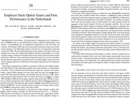
One special feature of ESOs is that they usually take several years to vest, within which no exercise is allowed. Case one and two value repriceable options as if they were European options. This numerical solution allows the option to have a vesting period for part of the option life, and the option becomes a combination of European and American option. Assume the vesting period is 4 years for a 10 year option. After the vesting period, option holders might choose to exercise the option when it is optimal to do so, or when the option holders face liquidity constraints. We first value repriceable ESOs allowing only one resetting. One complicated feature of this case is that endogenous exercise itself is influenced by the forfeiture rate, exogenous exercise rate, underlying stock price and whether the reset event has happened. We investigate first how endogenous exercise changes with other variables. Then we study how option values change with forfeiture, exogenous exercise, endogenous exercise and reset events. Two exercise regions are produced by numerical solution step 3(b) and 4(b) according to boundary condition (7). Because the resetting event is path-dependent, the exercise region is also path-dependent. Assume the stock price hits the resetting barrier at τ ∈ [0, T ] for the first time , 15
S 320.00 312.00 304.00 296.00 288.00 280.00 272.00 264.00 256.00 248.00 240.00 232.00 224.00 216.00 208.00 200.00 192.00 184.00 176.00 168.00 160.00 152.00 144.00 136.00 128.00 120.00 112.00 104.00 96.00
.................................................8 .................................................8 .................................................8 ................................................88 ...............................................888 ..............................................8888 .............................................88888 ...........................................8888888 ..........................................88888888 ........................................8888888888 .....................................8888888888888 ....................................88888888888888 ....................................88888888888888 ....................................88888888888888 .....................................8888888888888 .......................................88888888888 .........................................888888888 ..........................................88888888 ............................................888888 .............................................88888 ..............................................8888 ...............................................888 .................................................8 .................................................8 .................................................8 .................................................8 .................................................8 .................................................8 ..................................................
0 τ T Figure A: The grid points between [0, τ] are the exercise indicators for repriceable option before the resetting barrier is reached.
S 208.00 200.00 192.00 184.00 176.00 168.00 160.00 152.00 144.00 136.00 128.00 120.00 112.00 104.00 96.00 88.00 80.00 72.00 64.00 56.00
.................................................8 .................................................8 .................................................8 .................................................8 ................................................88 ..............................................8888 ............................................888888 .........................................888888888 .....................................8888888888888 ....................................88888888888888 ....................................88888888888888 ......................................888888888888 ..........................................88888888 ............................................888888 ..............................................8888 ................................................88 .................................................8 .................................................8 .................................................8 ..................................................
0
τ
T
Figure B: The grid points between [τ, T] are the exercise indicators for repriceable options after the resetting barrier is reached
S 320.00 312.00 304.00 296.00 288.00 280.00 272.00 264.00 256.00 248.00 240.00 232.00 224.00 216.00 208.00 200.00 192.00 184.00 176.00 168.00 160.00 152.00 144.00 136.00 128.00 120.00 112.00 104.00 96.00
.................................................8 .................................................8 .................................................8 ................................................88 ...............................................888 ..............................................8888 .............................................88888 ...........................................8888888 ..........................................88888888 ........................................8888888888 .....................................8888888888888 ....................................88888888888888 ....................................88888888888888 ....................................88888888888888 .....................................8888888888888 ......................................888888888888 ........................................8888888888 ..........................................88888888 ............................................888888 .............................................88888 ..............................................8888 ...............................................888 .................................................8 .................................................8 .................................................8 .................................................8 .................................................8 .................................................8 ..................................................
0
T
Figure C: The exercise indicators for non-repriceable options Figure 2: Exogenous exercise rate = 0. Endogenous exercise occurs in region filled with 8, postponement in region filled with ‘.’.
S 320.00 312.00 304.00 296.00 288.00 280.00 272.00 264.00 256.00 248.00 240.00 232.00 224.00 216.00 208.00 200.00 192.00 184.00 176.00 168.00 160.00 152.00 144.00 136.00 128.00 120.00 112.00 104.00 96.00
.................................................8 .................................................8 .................................................8 ................................................88 ...............................................888 .............................................88888 ............................................888888 .........................................888888888 ......................................888888888888 ................................888888888888888888 ....................888888888888888888888888888888 ....................888888888888888888888888888888 ....................888888888888888888888888888888 ....................888888888888888888888888888888 ....................888888888888888888888888888888 ....................888888888888888888888888888888 ...................................888888888888888 ........................................8888888888 ...........................................8888888 .............................................88888 ..............................................8888 ...............................................888 ................................................88 .................................................8 .................................................8 .................................................8 .................................................8 .................................................8 ..................................................
0
τ
T
Figure A: The grid points between [0, τ] are the exercise indicators for repriceable option before the resetting barrier is reached. S 216.00 208.00 200.00 192.00 184.00 176.00 168.00 160.00 152.00 144.00 136.00 128.00 120.00 112.00 104.00 96.00 88.00 80.00 72.00 64.00 56.00
.................................................8 .................................................8 .................................................8 .................................................8 .................................................8 ...............................................888 .............................................88888 ..........................................88888888 ....................................88888888888888 ....................888888888888888888888888888888 ....................888888888888888888888888888888 ....................888888888888888888888888888888 ....................888888888888888888888888888888 ......................................888888888888 ...........................................8888888 ..............................................8888 ................................................88 .................................................8 .................................................8 .................................................8 ..................................................
τ
T
Figure B: The grid points between [τ, T] are the exercise indicators for repriceable options after the resetting barrier is reached
S 320.00 312.00 304.00 296.00 288.00 280.00 272.00 264.00 256.00 248.00 240.00 232.00 224.00 216.00 208.00 200.00 192.00 184.00 176.00 168.00 160.00 152.00 144.00 136.00 128.00 120.00 112.00 104.00 96.00
.................................................8 .................................................8 .................................................8 ................................................88 ...............................................888 .............................................88888 ............................................888888 .........................................888888888 ......................................888888888888 ................................888888888888888888 ....................888888888888888888888888888888 ....................888888888888888888888888888888 ....................888888888888888888888888888888 ....................888888888888888888888888888888 ....................888888888888888888888888888888 ....................888888888888888888888888888888 ..................................8888888888888888 ........................................8888888888 ...........................................8888888 .............................................88888 ..............................................8888 ...............................................888 ................................................88 .................................................8 .................................................8 .................................................8 .................................................8 .................................................8 ..................................................
0
T
Figure C: The exercise indicators for non-repriceable options Figure 3: Exogenous exercise rate = 0.4. Endogenous exercise occurs in region filled with 8, postponement in region filled with ‘.’. The endogenous early exercise region in Figure A is smaller than that of Figure C because the option holder postpones the exercise of the repriceable option. The endogenous exercise happens earlier and at lower stock price in Figure B, because once the exercise price has been lowered, the option holder is more likely to bring the option to early exercise.
the exercise region before τ is given by step 4(b), and the exercise region after τ is produced from step 3(b). Because time τ is uncertain, we can not combine the two exercise regions into one. Let the exogenous exercise rate take different values. We examine how exercise regions change with the exogenous exercise rates. Without losing generality, the reset barrier used equals 60% of the original exercise price. Two sets of exercise regions are presented for two exogenous exercise rates in Figure 2 and 3. The exercise regions for repriceable options are given by the combination of Figure A and B for each case. The exercise regions for equivalent non-repriceable options are shown in Figure C. Three interesting properties are revealed by these exercise regions. First, the endogenous early exercise region in Figure A is smaller than that of Figure C. The intuition behind this is that since the repriceable option has the opportunity to be repriced, the option holder holds the repriceable option longer. Second, after repricing, the endogenous exercise happens earlier and at lower stock price in Figure B. This is because once the exercise price has been lowered, the rational exercise choice of the option holder will change accordingly. Lastly, the endogenous early exercise regions are wider when the exogenous exercise rate is higher. The increase of the possibility of exogenous exercise also increases the likeliness of endogenous exercise. Table 4 reports the option values under no resetting and under 50% and 60% resetting barriers. For any given repricing barrier, ESO values decrease with the increase of exogenous exercise rate. h
0
5%
10%
15%
20%
22.79
22.56
Option value No resetting
23.80
23.41
23.07
ρ = 60
26.07 9.5% 25.63 9.5%
25.26
9.5%
24.94
9.4%
24.67
9.4%
ρ = 50
24.93 4.7% 24.48 4.6%
24.11
4.5%
23.79
4.4%
23.52
4.3%
Table 4: ESO value with single resetting and partial vesting. The percentage number indicates the percentage increases of option value created by resetting for a variety of possible values of exogenous exercise rate. When the resetting barrier is 60% of the original exercise price, the option value increases by approximately 9.5%. When the resetting barrier is 50% of the original exercise price, the option value increases by approximately 4.5%. 16
Although the percentage increases of option value changes with the level of the exogenous exercise rate, the variation is not big. A similar numerical experiment conducted by Corrado et al./ shows that the percentage change of option value is very sensitive to the choice of risk-aversion and nonoption wealth5 . This comparison shows that the result of intensity-based model is less sensitive to parameter values.
4.4
Case Four: ESOs with Multiple Resetting and Partial Vesting
In the last numerical experiment, other than partial vesting, forfeiture and exogenous early exercise, we assume the ESO exercise price will be reset up to four times whenever the stock price drops to ρ% of the original exercise price. The value of the options with ρ = 60 and ρ = 50 are calculated and reported in Table 5. h
0
5%
10%
15%
20%
22.79
22.56
Option value No resetting
23.80
23.41
23.07
ρ = 60
26.49 1.6% 26.02 1.5%
25.62
1.4%
25.29
1.4%
25
1.3%
ρ = 50
25.01 0.3% 24.56 0.3%
24.18
0.3%
23.86
0.3%
23.58
0.3%
Table 5: ESO value with multiple resetting and partial vesting Comparing the values of multiple resetting options to those of the single resetting options, the percentage increase is not very significant. As the number beside option value shows, the increase is about 1.5% when ρ = 60. The increase is only approximately 0.3% when ρ = 50. The increase of option value caused by multiple resetting is much smaller compared with the option value increase reported in Table 3. The key element causes this difference is that the option holder in this case is allowed to exogenously and endogenously early exercise and the early exercise reduces the potential gain from multiple resetting over single resetting. 5
Table 4 of Corrado et al. (2001).
17
5
Conclusion
It has become a common practice for firms to reduce the strike price on previously awarded ESOs when the stock price of the firm decreases significantly. With the repriceable feature being justified by the theoretical model as an effective corporate strategy to realign the interests of employees to those of shareholders, one problem to be solved about repriceable ESOs is to value the cost of repriceble ESO so that this cost could be correctly reflected in the firms accounting report. Few papers have discussed valuation models applicable to repriceable options, and the models used in the former literature are based on the Barrier Option formula, which overvalues ESOs because it can not incorporate most of the special features of ESOs. This paper develops an intensity-based model to asses the cost of repriceable ESOs, which reflects most of the special features of repriceable ESOs. The model is applied to evaluate the cost of several types of repriceable options. We also examine how the value and the exercise decision are affected by single or multiple resetting. Three conclusions about resetting are reached by the study. First, consistent with the former research, we find that the value of repriceable options first increase with the decrease of resetting barrier, then decrease with the decrease of resetting barriers. Second, multiple resetting increases option value more than single resetting does, but the size of difference is not significant. Lastly, the resetting provision postpones the exercise decision of the option holders before resetting. But once the exercise price has been reset, option holders are more likely to bring the option to exercise. The model developed here extends the literature by three aspects. First, this is the first attempt to use intensity-based framework to value repriceable option. It overcomes several disadvantages of the existing models. Furthermore, the valuation model incorporates most of the special features of ESOs. Second, it is shown that although the repriceble ESOs cost more to shareholders than non-repriceable ESOs, the cost is lower than B-S valuation result. Lastly, the model gives out the exercise patterns of the repriceable options, which can be used for further investigations on the incentive effect of repriceable options.
18
References [1] Acharya, V. V., John, K., Sundaram, R. K., 2000. On the optimality of resetting executive stock options. Journal of Financial Economics 57, 65-101. [2] Brenner, M., Sundaram, R. K., Yermack, D., 2000. Altering the terms of executive stock options. Journal of Financial Economics 57, 103-128. [3] Carpenter, J. N., 1998. The exercise and valuation of executive stock options. Journal of Financial Economics 48, 127-158. [4] Carr, P., Linetsky, V., 2000. The valuation of executive stock options in an intensity-based framework. European Finance Review 4, 211-230. [5] Chance, D. M., Kumar, R., Todd, R. B., 2000. The “repricing ”of executive stock options. Journal of Financial Economics 57, 129-154. [6] Corrado, C. J., Jordan, B. D., Miller, T. W., Stasfield, J. J., 2001. Repricing and employee stock option valuation. Journal of Banking & Finance 25, 1059-1082. [7] Detemple, J., Sundaresan, S., 1999. Nontraded asset valuation with portfolio constraints: a binomial approach . The Review of Financial Studies 12, 835-872. [8] Duffie, D., Huang, M., 1996. Swap rates and credit quality. Journal of Finance 51, 921-49. [9] Duffie, D., Singleton, K., 1997. An econometric model of the term structure of interest-rate swap yields. Journal of Finance 52, 1287-321. [10] Duffie, D., Singleton, K., 1999. Modeling term structures of defaultable bonds. Review of Financial Studies 12, 687-720. [11] Gilson, S. C., Vetsuypens, M. R., 1993. CEO compensation in financially distressed firms: an empirical analysis. The Journal of Finance 48, 425-458. [12] Hart, O., Moore, J., 1988. Incomplete contracts and renegotiation. Econometrica 56, 755-785. [13] Huberman, G., Kahn, C., 1988. Limited contract enforcement and strategic renegotiation. American Economic Review 78, 471-484. 19
[14] Huddart, S., 1994. Employee stock options. Journal of Accounting and Economics 8, 23-42. [15] Hull, J., White, A., 1993. Efficient procedures for valuing European and American pathdependent options. Journal of Derivatives Fall, 21-31. [16] Hull, J., White, A., 2003. Accounting for employee stock options. Working paper, Rotman School of Management, University of Toronto [17] Jarrow, R. A., Lando, D., Turnbull, S., 1997. A Markov model for the term structure of credit spreads . Review of Financial Studies 10, 481-523. [18] Jennergren, L., Naslund, B., 1993. A comment on “ valuation of executive stock options and the FASB proposal ”. The Accounting Review 68, 179-183. [19] Kulatilaka, N., Marcus, A., 1994. Valuing employee stock options. Financial Analysts Journal November-December, 46-56. [20] Rubinstein, M., Reiner, E., 1991. Breaking Down the Barriers. Risk September, 28-35. [21] Saly, P. J., 1994. Repricing executive stock options in a down market. Journal of Accounting and Economics 18, 325-356. [22] Johnson, S. A., Tian, Y. S., 2000. The value and incentive effects of nontraditional executive stock option plans. Journal of Financial Economics 57, 3-34.
20