Ozone Monitor Network Options. 1111 with the other policy alternatives when uncertainties are present. Learning-based approaches have been advocated.
Risk Analysis, Vol. 25, No. 5, 2005
DOI: 10.1111/j.1539-6924.2005.00666.x
How Much Uncertainty is Too Much and How Do We Know? A Case Example of the Assessment of Ozone Monitor Network Options Cynthia H. Stahl1 ∗ and Alan J. Cimorelli1
Limited time and resources usually characterize environmental decision making at policy organizations such as the U.S. Environmental Protection Agency. In these climates, addressing uncertainty, usually considered a flaw in scientific analyses, is often avoided. However, ignoring uncertainties can result in unpleasant policy surprises. Furthermore, it is important for decisionmakers to know how defensible a chosen policy option is over other options when the uncertainties of the data are considered. The purpose of this article is to suggest an approach that is unique from other approaches in that it considers uncertainty in two specific ways—the uncertainty of stakeholder values within a particular decision context and data uncertainty in the light of the decision-contextual data–values relationship. It is the premise of this article that the interaction between data and stakeholder values is critical to how the decision options are viewed and determines the effect of data uncertainty on the relative acceptability of the decision options, making the understanding of this interaction important to decisionmakers and other stakeholders. This approach utilizes the recently developed decision analysis framework and process, multi-criteria integrated resource assessment (MIRA). This article will specifically address how MIRA can be used to help decisionmakers better understand the importance of uncertainty on the specific (i.e., decision contextual) environmental policy options that they are deliberating. KEY WORDS: Environmental decision making; policy analysis; precautionary principle; uncertainty
1. THE PROBLEM
dence level. Inherent uncertainty is the focus of precautionary principle advocates and practitioners and represents unknowns that cannot be further reduced. Since this type of uncertainty cannot be eliminated with more information or better science, many choose to ignore it. As difficult as these two types of uncertainty are to address, policy decision making is even more complex. Policy making is not just a compilation of data or an acknowledgment of inherent real-world uncertainty but rather it must integrate data with values in the light of uncertainties. The relationship between the data and values is a critical component of decision making. However, the importance and influence of data-value relationships within specific decision-making contexts is often minimized
Uncertainty is generally thought of in two major ways—as data/model uncertainty and as inherent uncertainty. Data/model uncertainty is most often addressed by scientists because this is where they apply their expertise. The goal is to reduce this uncertainty to within a realm considered acceptable to their scientific discipline. For example, this could mean the application of the statistical 95% confiU.S. Environmental Protection Agency, 1650 Arch Street, Philadelphia, PA 19103, USA. ∗ Address correspondence to Cynthia H. Stahl, U.S. Environmental Protection Agency, Region III, 1650 Arch St., Philadelphia, PA 19103. 1
1109
C 2005 Society for Risk Analysis 0272-4332/05/0100-1109$22.00/1 �
1110 or overlooked. These relationships are typically revealed in situations where decisionmakers note that stakeholders fail to appreciate the rationale for their final decision, where unexpected impacts (or surprise responses) occur, or accusations of manipulating data for a desired result are made (Thompson, 1983; Gerrard, 2000; Lynn, 1990; Cranor, 1997; Charnley, 2000; Krimsky & Plough, 1988). Therefore, understanding the data-value relationships is important to informing decisionmakers and other stakeholders for better decision making. For example, while knowing air quality levels may be important for a decision about whether the air quality in an area is good or not and may also be important for a decision about whether to approve an industrial source permit, the air quality information may not necessarily carry the same importance for both of these decisions. This is because the relationship between data (air quality) and values (how important is air quality to the specific decision) can be different for two different decision contexts. Even when the data-values relationships are acknowledged in policy making, current methodologies do not provide insight to decisionmakers about how data/model uncertainties and inherent uncertainties may interact with those relationships. However, knowing how much uncertainty a decision can tolerate helps to inform the decisionmaker about the decision. She may find that once uncertainties are considered, the original policy choice is less attractive now and she may change her mind and decide to choose a different policy option. Furthermore, she may also test the effect of uncertain values with uncertainties on the relative attractiveness of the policy options. Defining, testing, and learning about the interaction of data, values, and uncertainties needs to become part of the policy analysis. Even when uncertainty is discussed, policy analysts attempt to limit its consideration, address only uncertainties in specific pieces of data, indicate that uncertainties may be very large and produce impacts to the final conclusion that are not part of the analysis, or, in other cases, list the assumptions of the analysis so as to avoid specifically addressing some troubling uncertainties (U.S. Environmental Protection Agency et al., 1999; U.S. Department of Energy, 2004; U.S. Environmental Protection Agency, Office of Pollution Prevention and Toxics, 1998; U.S. Environmental Protection Agency, Office of Research and Development and U.S. Environmental Protection Agency, Office of Solid Waste, 2003; U.S. Environmental Protection Agency, 1999; U.S. Department of Energy, 2004; U.S. Environmental Protection Agency, Office of Air and
Stahl and Cimorelli Radiation, Air Quality Strategies and Standards Division, Emission, Monitoring and Analysis Division, Clean Air Markets Division, 2005). In most cases, discussions of uncertainty in policy analysis, when it is present, is limited to data uncertainty or model uncertainty. Inherent uncertainties of the system, the focus of precautionary principle advocates, are rarely discussed or addressed. The influence of the data-values relationships on the acceptability of uncertainties for any particular decision is considered even less frequently. The interaction between data and values is unique to the decision context and its understanding is important to decisionmakers and other stakeholders because environmental policy decisions are rarely about just data or values. This article explores the data-values relationships in a case study of ozone monitoring network options. Furthermore, this case study is used to illustrate how uncertainties can be examined in a new way that would allow decisionmakers and other stakeholders to better understand the impact of the interaction among data, values, and uncertainties on the relative acceptability of the decision options. Precautionary principle advocates, in particular, stress the importance of acknowledging uncertainty in environmental policy decisions in order to avoid unpleasant surprises. However, even when the consideration of uncertainty is acknowledged as important, practitioners have been stymied with regard to how to determine uncertainties’ impact on policy options. In policy analysis, decisionmakers want to know whether they would make a different policy choice if the data were different than initially presented or assumed. In order to determine uncertainties’ impacts on policy options, it is first necessary to consider stakeholder values, the certainty of these stakeholder values pertaining to the particular decision being discussed, what the relationship is between the data and these values, and, finally, how uncertainties together with the data-values relationship influence the stakeholders’ views regarding the attractiveness of the policy options. This article shows that, when value sets are compared using the same data, data uncertainty can alter the acceptable decision option. This is because data uncertainty has a greater influence on the decision options in some value sets compared to other value sets. Therefore, it is important for decisionmakers to understand the interplay between data uncertainty and the uncertainty of stakeholder values. Decisionmakers can find it difficult to defend the chosen policy option when challenged by opponents if they do not know how that option fares in comparison
Ozone Monitor Network Options with the other policy alternatives when uncertainties are present. Learning-based approaches have been advocated by public policy theorists and practitioners (Innes de Neufville & Christensen, 1980; Hisschemoller & Hoppe, 2001; Schon, 1971; Harremoes et al., 2001; Van Groenendaal, 2003; Finger & Verlaan, 1995; Lee, 1993). For each of these learning advocates, learning allows the incorporation of different goals so that all the important decision aspects are reflected in the final decision. In environmental public policy making, physical science data is important but often, as controversial decisions reveal, not to the exclusion of social values. When the decision-making process includes a learning component, all stakeholders benefit by better understanding the relationships between the data and values. Unfortunately, however, many decision analysis tools tend to shortcut the learning process through optimization, oversimplification, or limiting discussions to experts. When time and resources are limited, the problem of truncated learning is exacerbated. Limited time and resources in policy-making organizations such as the U.S. Environmental Protection Agency often require decision-making triage. While the decisionmaker, in these cases, wants to know whether the uncertainties in both the data and stakeholder values support making a different policy choice (or weaken the justification of the favored option) or result in the creation and consideration of different policy alternatives, she also needs to know whether additional time and resources should be spent on more precisely defining those data/model uncertainties in a statistically vigorous manner. 2. THE SOLUTION A possible solution to this problem is a transparent, learning-based process that allows stakeholders, including decisionmakers, to examine how uncertainty affects policy choices. Such a methodology has been developed at the U.S. Environmental Protection Agency. The multi-criteria integrated resource assessment (MIRA) approach was used to evaluate decision alternatives pertaining to the designations of geographic areas for the 1-hour ozone standard and the 8-hour ozone standard (Stahl, 2003; U.S. Environmental Protection Agency, Office of Air Quality Planning and Standards, 2004; Stahl et al., 2004). Typically, current decision analytic methods that consider uncertainty limit this aspect to data uncertainty and sensitivity analysis pertaining to data un-
1111 certainty. These methods often fail to consider the importance of stakeholder values and the influence that these values have on how data uncertainty is viewed with respect to the relative acceptability of the decision alternatives. Specifically, the failure to consider stakeholder values within an analysis that includes data (and its commensurate uncertainties) is a failure to consider decision context. In these cases, decision analysts perform their analyses outside of the decision context. Consequently, surprises regarding the impacts of the chosen decision option, as well as the responses of the stakeholders to the decision, can result. For example, in multiattribute utility theory (MAUT) methods, the creation of a willingness-topay utility function is a one-time input to the analysis that independently establishes the relationship between willingness to pay and pollution controls. Furthermore, current decision analytic methods do not specifically allow decisionmakers to examine the interplay between data uncertainty and variations in stakeholder values in order to determine how stakeholder values influence the acceptability of data uncertainty in some cases but not in others. In contrast, in the MIRA approach, decision context is used to guide the user to better understand data-values relationships and the relationship between data, data uncertainty, and stakeholder values. When data relationships such as the MAUT utility functions are established outside of a decision context, the analysis may lose relevance. For example, it is possible to ask an industrial stakeholder whether she might be willing to spend $1 to install pollution controls on her new manufacturing facility to control toxic emissions. Let us suppose that she agrees to spend $1 and, as we continue to question her in stepwise fashion, is willing to spend up to $1,000 on pollution controls but is not willing to spend $1,001. Suppose that we now tell the industrial stakeholder that her parents live in the area that will be downwind from her manufacturing facility and ask her again whether she is willing to spend more than $1,000 on pollution controls. It is likely that her answer will change because the context is changed even though the cost of pollution controls and all other aspects of her manufacturing facility remain the same. However, this does not mean that the use of a MAUT utility function is, in all cases, inappropriate. In fact, a decisionmaker may conclude that the use of the utility function is most appropriate, given the particular decision context. If this is the case, the values/preferences inherent within the utility function can be utilized within the MIRA framework. The explicit incorporation of
1112 decision context is an important difference between MIRA and other decision analytic approaches. A detailed description of MIRA’s concepts and the MIRA process can be found in Stahl et al. (2002) and Stahl (2003). Just as establishing a utility function out of context could result in an irrelevant analysis, making presumptions about the importance of data uncertainty out of the decision context can be just as fallacious. When the importance of data uncertainty is determined within a decision context, decisionmakers and other stakeholders are more completely informed about the decision problem and the relationship between the data and the decision options. It is the premise of this article that if decisionmakers first learn about the data-values relationships and use this understanding to explore the effects of uncertainty on decision options, policy decisions can be more supportable and scarce time and resources can be better allocated to only those situations that call for more precise data/model uncertainty estimates. In a MIRA-based decision analysis, decisionmakers have the advantage of examining uncertainty in a manner that allows them to consider the interplay between data uncertainty and the decision-contextual data– values relationships. The implication for policy analysts is that learning about the effect of uncertainty becomes part of the analytical process. As part of this process, a variety of stakeholder inputs, including issues of data uncertainty and values uncertainty, can be examined and the impact of these inputs can be assessed. When this kind of feedback loop is utilized in the analytical process, stakeholders can see directly how their concerns are being considered and decisionmakers can show how they are being responsive to these stakeholder concerns. Furthermore, time can be saved by a process that allows decisionmakers to avoid starting the analysis from the beginning each time stakeholders may react adversely to that decision. 3. THE MIRA METHODOLOGY/PROCESS The MIRA analytical methodology allows stakeholders to organize decision criteria hierarchically and connect these criteria to data. This allows for the link between data, criteria, and policy options to be explicitly presented. Within the MIRA approach, stakeholders work with decisionmakers toward answering a specific policy question, which may involve determining what kinds of policy options are available and which policy option best fits with the decision crite-
Stahl and Cimorelli ria. Decisionmakers and other stakeholders work together in identifying important decision criteria and the data associated with them. These criteria are transparently organized in the MIRA framework and the analysis begins by first initializing the relative significance of the criteria data to the specific policy question being deliberated.2 The MIRA methodology offers stakeholders the ability to index these otherwise disparate criteria and data onto a common decision scale for the direct comparison of criteria and their data in the policy context. Typically, a numeric scale between 1 and 8 is used to indicate the relative significance of the criteria data to the policy decision. Indexing places the criteria and data into the policy context and, through this, the significance of the individual criteria data can be openly discussed among the stakeholders. Certain criteria data, such as the significance of health impacts due to ozone exposure or the costs of particular kinds of pollution controls, may require input from expert stakeholders. The iterative nature of the MIRA methodology encourages experimentation with indexing in order to allow stakeholders to better understand the relationship between the criteria data and the policy alternatives being discussed. The MIRA process also contains a procedure for the incorporation of stakeholder values. Separate from the indexing procedure, values incorporation occurs when stakeholders determine the relative importance of the decision criteria.3 Six different preference schemes/value sets are examined in this article. The capability to examine the specific interaction between these value sets and data uncertainty is a unique attribute of MIRA and the focus of this article. In the MIRA methodology, indexed criteria data are multiplied by a set of criteria weights in a preference scheme, resulting in the ranking of policy alternatives from most to least preferred. Again, as with indexing, there are no right preferences and stakeholders are encouraged to experiment with different preference schemes (i.e., value sets) in order to learn about the effect that different values have on the policy alternatives. Iteration is an important part of the MIRA-guided policy analysis process. The initial identification of criteria and data starts the process and it is expected that decisionmakers and stakeholders will return to this step in order to add, modify, or change criteria as their understanding of the analysis and decision options improves. 3 Indexing can be thought of as the primary area where experts apply their expert knowledge to the significance of data. In contrast, determining the relative importance of decision criteria can be thought of as the primary area where stakeholder values are considered. 2
Ozone Monitor Network Options
1113
4. THE CASE STUDY In order to demonstrate the feasibility of using MIRA in addressing the role of uncertainty, a case example of the evaluation of the ozone monitoring network in the U.S. Mid-Atlantic region is used. In this case study, policymakers want to know whether the current network of ozone monitors in the U.S. MidAtlantic is adequate for making estimates of ozone levels in the region. While it is intuitively always better to have more ozone monitors rather than less, the costs to establish and operate the network must be balanced against more and more accurate estimates of ozone levels. Ozone level estimates are used to make major policy decisions at the U.S. EPA with regard to emission control strategies and air quality planning. It is a dilemma of the U.S. EPA decisionmakers to balance extremely accurate monitoring data with the costs of obtaining such data. Which monitoring network option would allow the U.S. EPA to get the best monitoring data at the least cost? Through this case study, we show that it is not just a matter of optimization to answer this question but an understanding of the values being used to make such judgment that influences which option is considered acceptable. The ozone monitoring network in this region currently consists of 110 monitors located primarily in
urban areas. The location of these monitors has historically been determined by concerns for the exposure of human populations to unhealthy levels of groundlevel ozone, which can cause or exacerbate respiratory problems, particularly in children and the elderly. However, while the emphasis has been on human populations, the information obtained by the ozone monitoring network is also used to assess ozone levels in rural areas, on sensitive ecosystems, and to determine the contribution of ozone precursor emissions on downwind areas exhibiting poor ozone air quality. Because ozone monitoring data is used for these varieties of purposes, when an evaluation of the monitoring network adequacy is conducted, it is important that multiple criteria be used. In this case study, we examine a few of these possible criteria and experiment with the effect of data uncertainty on the potential acceptability of three network options.
5. THE EXPERIMENTAL APPROACH A total of 14 criteria are used in this case example of ozone monitoring networks. These criteria are arranged hierarchically (Fig. 1). The criteria at the primary level are: ozone air quality, personnel impact, costs, and air quality trends. The ozone air quality Description of Statistics
PRIMARY LEVEL
SECONDARY LEVEL
1-Hr O3 Nonattainment Areas
Ozone Air Quality
TERTIARY LEVEL
Data Fit
Area Wide Population Weighted
Data Scatter
Area Wide Population Weighted
Worst Outlier
1-Hr O3 Attainment Areas
Data Fit
Area Wide Population Weighted
Data Scatter
Area Wide Population Weighted
Worst Outlier Personnel Impact
QUATERNARY LEVEL
Monitor Servicing Distance Workload
Costs Trends Impact
Fig. 1. Ozone monitoring network assessment criteria.
1114 criterion considers the air quality in urban (in general, areas that are currently designated by the U.S. Environmental Protection Agency as 1-hour ozone nonattainment areas)4 versus rural areas (areas that are currently designated by the U.S. Environmental Protection Agency as 1-hour ozone attainment areas). Further, the ozone air quality criterion contains subcriteria that allow for the consideration of the adequacy of a network’s spatial distribution of monitors to allow for the accurate estimate of air quality via interpolation. The statistics used are the absolute fractional bias (data fit), the square of the correlation coefficient (data scatter), and the 95th percentile residual (worst outlier). The consideration of absolute fractional bias and the square of the correlation coefficient can also be assessed with respect to population and to the area overall (i.e., urban or rural). The breakdown of the ozone air quality criterion in four hierarchical levels permits the analyst to examine components of the ozone monitoring network decision with respect to specific areas of interest. The personnel impact criterion is included in the analysis in order to capture the personnel cost in maintaining each of the three possible network configurations. The personnel impact criterion has two subcriteria: monitor servicing distance, which is the distance between the monitor and the nearest office of the state air quality agency, and workload, which is the number of ozone monitors per state monitoring staff. The cost criterion considers capital costs and operation and maintenance (O/M) costs for the ozone monitors. The air quality trends criterion captures the importance of having historical monitoring data at the same location in order to evaluate longterm ozone exposure. The air quality trends criterion considers the length of the monitoring record at each ozone monitoring site. Using this metric, stakeholders can weigh more heavily the removal of existing ozone monitors with long historical records since it may be important to have air quality information at the same site over a period of time in order to assess long-term exposure impacts. Each of these criterion help the 4
Areas designated by the U.S. Environmental Protection Agency as nonattainment under the 1-hour ozone standard of 0.12 ppm are not meeting this national, health-based ozone standard. Conversely, areas that are designated ozone attainment are meeting this ozone standard. EPA has updated the national ambient air quality standard for ozone to a more stringent 8-hour standard of 0.08 ppm. The new 8-hour ozone nonattainment areas are similar but generally slightly larger than the 1-hour ozone nonattainment areas. At the time this case study was prepared, the 8-hour ozone nonattainment areas had not yet been determined.
Stahl and Cimorelli decisionmaker to evaluate whether the current ozone monitoring network is adequate with respect to accurate monitoring data, resource constraints, and costs. In this study, the base case (the current ozone monitoring network) is compared with two new monitoring network options, identified as least cost (LC) and best kriging estimate (BKE). While many different monitoring network options can be tested, for simplicity, this article discusses only three network options, including the status quo . The LC option starts with the current ozone monitoring network of 110 monitors and removes a total of 62 monitors without significantly reducing the quality of the ozone air quality estimate5 for the U.S. Mid-Atlantic region overall.6 The BKE option starts with the LC option of 48 monitors and adds ozone monitors judiciously in locations that are likely to produce the greatest improvement in the ozone air quality estimate. In this option, four new ozone monitors are added over the LC option. Two of these ozone monitors are in completely new locations (i.e., no monitors for any pollutant exist at these sites). The remaining two new ozone monitors are added to sites that currently contain other pollutant monitors. For this case example, potential data uncertainties are examined with respect to two data variables: ozone analyzer O/M costs and monitoring station O/M costs.7 This article will illustrate the possibility of bracketing the effect of data uncertainties in these two criteria so that analysts and other stakeholders can learn about the impacts of data uncertainty on the three network options within Ozone air quality is monitored at select, primarily urban, locations throughout the Mid-Atlantic region during the ozone season, which usually runs from May 1 through September 30. Estimating ozone air quality everywhere in the Mid-Atlantic requires using these monitoring data and interpolating them to produce air quality estimates in locations where there are no ozone monitors. Kriging, used in this study, is one accepted method of interpolation. The interpolated air quality estimate is compared to the accepted state-of-the-art modeled field of air quality (benchmark) estimates and statistics are used to compare the fits of these two interpolated fields. 6 Significance is defined in the following manner. To obtain the least cost network, 62 monitors are removed from the current monitoring network configuration (base case). The interpolated air quality estimates for the LC network are determined not to deviate significantly from the base network’s air quality estimates if they remain within 2% of the benchmark concentrations (as calculated by the absolute fractional bias), and there is less than 5% degradation in the variance when compared to the base network. 7 Given the three network options, capital costs affect only the BKE option (two new stations at $50,000/station) and so, given this simple case example, changes in capital cost do not result in altering the rankings of BKE relative to LC or B until these capital costs are exceeded by O/M costs. 5
Ozone Monitor Network Options
1115
the context of different value sets. This means that decisionmakers/stakeholders can determine when and where data uncertainties affect the possible ranking and choice of policy options and can approach scientists/statisticians with specific questions about whether certain critical pieces of data are likely to approach these uncertainty levels that affect the choice of policy options. This is the reverse of what is typically demanded of scientists and statisticians but it is our premise that this reversal will allow for the more efficient utilization of scientific data into environmental policy decision making. In addition, this allows managers to more strategically target resources where they are needed. We begin by first presuming that the data are certain and produce a ranking of the three possible network options using an initial value set. Next, we examine the possibility that some of the cost data are uncertain (using the same value set), experimenting with ranges of uncertainty, and examining the resulting relative option rankings.
By first assuming that the data is certain, the MIRA-guided evaluation of the three network options produces a cardinal ranking of these options: BKE, LC, and base. Although there are many different preference schemes (i.e., value sets) that can produce a cardinal ranking where the BKE option is ranked most optimal, followed by LC and then the base (B) option, we select six different preference schemes (or value sets) at the primary criteria level for examination (see Table I). Table I shows just a few combinations of the wide variety of possible preference weights that produce the same cardinal ranking of options. The fractions represent the portion of the decision pertaining to monitoring network options relative to air quality, personnel impact, costs, and trends. The
fractions total to 1.0 or 100%. For example, air quality can represent 35% of the decision (Value Set 4) or 60% of the decision (Value Set 2) and, depending on the relative contributions of the other criteria, still produce the same cardinal ranking of options. This flexibility in criteria weights indicates a certain level of robustness with respect to the preference ranking of these options. The MIRA approach allows the analyst to use these criteria weights as part of the learning process in the evaluation of a particular decision; in this case, the evaluation of ozone monitoring network options. In a MIRA-guided analysis, the relative ranking of the decision options is determined by the calculation of criteria sums, defined as linear weighted sums of indexed criteria (weights provided through the preference schemes). While the absolute values of these criteria sums are not particularly important, the relative numeric values can be used to elucidate information about both the differences among the three network options as well as quantifying the differences among value sets, as they pertain to a particular decision option. The criteria sums of all three options for each of the six value sets in this study are shown in Table II. The difference in criteria sums between any two options can be interpreted as the degree to which one option is more attractive than another; or in the case of the first two ranked options, the degree of confidence that a decisionmaker might have in selecting the top ranked option. In general, decisionmakers want to know how much of a distinction there is between the first ranked option and the next option. If these criteria sums in Table II are compared as ratios, BKE/LC and BKE/B, the result can be graphically displayed in Fig. 2. In Fig. 2, the relative attractiveness of BKE is compared to LC and B for each of the six value sets. A decisionmaker can feel more confident about accepting the BKE option with Value Set 2 than with Value Set 1, where the difference from the next option is, relatively, much smaller. In other
Table I. Six Preference Schemes at the Primary Criteria Level
Table II. Criteria Sums for the Three Network Options for Six Preference Schemes
6. DATA IS CERTAIN
Preference Scheme
Air Quality
Personnel Impact
Costs
Trends
Preference Scheme
Best Kriging Estimate
Least Cost
Base
BKE/LC (%)
Value Set 1 Value Set 2 Value Set 3 Value Set 4 Value Set 5 Value Set 6
0.450 0.600 0.400 0.350 0.500 0.650
0.150 0.100 0.100 0.200 0.100 0.100
0.300 0.250 0.350 0.100 0.200 0.200
0.100 0.050 0.150 0.350 0.200 0.050
Value Set 1 Value Set 2 Value Set 3 Value Set 4 Value Set 5 Value Set 6
4.3904 4.7402 4.2589 3.3083 4.1206 4.7658
4.2699 4.3790 4.1404 3.2741 3.8391 4.3335
3.7098 4.1386 3.5982 3.2044 3.7744 4.2502
2.81 8.24 2.86 1.04 7.33 9.97
Percent Separation Between Options
1116
Stahl and Cimorelli 7. DATA IS UNCERTAIN
20% 15% 10%
Least Cost
5%
Base
0% 1
2
3
4
5
6
Value Sets
Fig. 2. Relative attractiveness of best kriging estimate option compared with least cost and base options.
words, the more value one places on the air quality impact of the decision, the more confident one can be in choosing the BKE option. Table II can also be used to examine the attractiveness of a single network option when compared among different value sets (i.e., compare criteria sums vertically rather than horizontally as previously done for Fig. 2). Higher criteria sums indicate greater strength or attractiveness of an option among the tested value sets (for a given data set and indexing). Therefore, while Value Set 2 provides the greatest justification for the LC option among all the value sets, Value Set 6 provides the greatest justification for the base option (4.25 is the highest criteria sum for the base option among the six value sets). This information can provide decisionmakers with the ability to better understand what mix of values might better support a particular option. For each of the three network options, Value Set 4 provides the least justification (i.e., lowest criteria sums). Using Value Set 4 as the benchmark, Fig. 3 offers a comparison of the three network options for each of the remaining value sets. This figure shows the variation in the degree of justification among the value sets and that Value Set 6 provides the greatest degree of justification for the BKE and B options among the six value sets examined while Value Set 2 provides the greatest degree of justification for the LC option.
In this section, we explore the effect of uncertain data on the assessment of the three network options. If the data are acknowledged to be uncertain, decisionmakers often want to know how the attractiveness of the options may change as a result of the spread in the data from uncertainty. Decision analysis in the light of new information is not simply a matter of adding data but also requires a reanalysis of the data and data relationships. MIRA allows for such a reanalysis. For this example, we vary O/M costs from the assumption used to produce the criteria sums in Table II (i.e., $16,000 per monitoring station and $3,400 per ozone analyzer (both in 1993 dollars)) as if we are uncertain about them. When these O/M costs are varied, the cardinal ranking of the options may change and this can be used to determine how much uncertainty in this variable can be tolerated before the decisionmaker believes that her initial choice should be changed. The MIRA approach is used to generate the relative criteria sums in the network options resulting from data changes designed to examine how sensitive the decision is to possible data uncertainty. However, whether the impact of uncertainty results in the conclusion that the decision option is justifiable or not is left to the decisionmaker. MIRA cannot make that determination. As the cost is varied in the MIRA analysis, stakeholders can examine how the relative acceptability of each decision option is affected for each value set. This is a key difference between MIRA and other existing methodologies where values are neither an integral nor an experimental part of the analysis. As a result, in these analyses, it is not possible to determine the interaction between data uncertainty and stakeholder values; nor is it possible to understand how the combination of these factors affects how favorably the decision options are viewed. This concept is further explained below.
Increase Above Least Justifiable Value Set
8. RESULTS 8.1. Preserving the Original Cardinal Ranking with Data Uncertainty
50% 40%
Best Krige
30%
Least Cost
20%
Base
10% 0% 1
2
3
5
6
Value Sets
Fig. 3. Variation in degree of justification among value sets.
One approach to defining what constitutes an acceptable amount of data uncertainty is to determine how much the data must change to produce changes in the original cardinal ranking of options. Data uncertainty of such magnitude could be considered unacceptable since it could support an entirely different decision. This may occur in situations where
Ozone Monitor Network Options
1117
the decisionmaker has already announced her decision at the end of an analysis that presumed the data was certain and, as a result of stakeholder comment, is reevaluating the decision based on data uncertainty. If the original cardinal rankings of the options change as a result of data uncertainty and if the uncertainty cannot be reduced, the decisionmaker could conclude that the decision options are indistinguishable. 8.2. Flexibility of Preference Schemes to Data Uncertainty Depending on the specific preference scheme chosen, some cost data changes alter the original cardinal order of the network options. In Fig. 4, the six value sets are compared with respect to the cost necessary to force the first change in the original cardinal ranking. As can be seen in this figure, Value Set 1 can accommodate more uncertainty (i.e., wider swing of cost estimates) in the station and analyzer O/M costs than any of the other five value sets. In general, the six value sets tolerate less uncertainty with respect to analyzer O/M cost uncertainty than station O/M cost uncertainty. The implications for the decisionmaker are that very uncertain data in some circumstances may not be important but a little data uncertainty in other circumstances may be critical. Under Value Set 4, BKE remains the most preferred option when O/M costs begin to vary but decisionmakers may want to know when (i.e., at what specific combinations of cost uncertainty) BKE would no longer remain the most preferred option. In order to understand whether and when the first ranked option changes as the data becomes more uncertain, an examination of different analyzer O/M costs and station O/M costs is conducted and this is shown in Fig. 5. Since the option with the maximum criteria sum is the first ranked option, if the maximum criteria sum is graphed for each combination of analyzer O/M cost and station O/M cost for a particular value set, the
O/M Costs
$50,000 $40,000 $30,000
Station
$20,000
Analyzer
$10,000 $0 1
2
3
4
5
6
Fig. 5. Top ranked option relative to O/M cost combinations (Value Set 4).
analyst can see at what combinations of analyzer and station O/M costs bring changes to the top ranked option.8 Although the base option will never, in absolute dollars, be cheaper than the BKE option, as O/M costs become lower, there is some point at which the decisionmaker has judged that the base cost is cheap enough for her to accept it as equivalent to or better than the BKE option. This judgment is reflected through the combination of the way the decisionmaker indexed the data and the choice of the value set. When she learns how that initial judgment affects the relative ranking of the options, the decisionmaker can determine whether she should try another index scale and/or another value set in the next iteration. Therefore, in this case study, when station O/M costs are low, the base option is favored because the relative amount of cost savings between the BKE and base options is less than what it was when the station O/M costs were higher. Since the analysis considers not just cost but other criteria, and cost is only 10% of the decision in Value Set 4, at lower station O/M costs, there are other factors that result in the base option becoming more favored than the cheaper BKE option. In Fig. 5, the BKE option is shown as the most preferred option when O/M station costs exceed $10,500
Value Set 8
Fig. 4. Minimum cost necessary to force rank changes among options.
Recall that the initial MIRA analysis was performed with best cost estimates of $16,000 for station O/M cost and $3,400 for analyzer O/M cost.
1118 over the full range of analyzer O/M cost uncertainty. Since the O/M station costs’ best estimate was $16,000 at the start of this study, the data in Fig. 5 supports the choice of the BKE option even when the O/M station costs are uncertain and substantially less than originally presumed. Because of the constraints initially placed on this analysis to limit the choice of demonstration value sets to those that result in the cardinal ranking of BKE, LC, and B, the analysis so far has been biased toward certain value sets that weigh the air quality criterion substantially more than the other criteria. However, a decisionmaker may want to know what circumstances could produce the LC option as the first ranked option. Value Set 7 is introduced here to illustrate how the three network option ranks flip more easily when the primary criteria weights are more equally balanced. Value Set 7 weighs the air quality, personnel, cost, and trends criteria at 25%, 15%, 30%, and 30%, respectively. Because the BKE option is designed to obtain an improved estimate of ozone air quality, the BKE option will be more favored as an option when the air quality criterion is weighted more heavily. Because the trends criterion is an indicator constructed to allow stakeholders to weigh the length of an existing monitor’s data record more heavily, the base option is more favored when the trends criterion is weighted more heavily. Therefore, with a preference scheme like Value Set 4, where the air quality criterion is not weighted as heavily as the others (35% vs. 45% or higher) and where the trends criterion is weighted more heavily than the other preference schemes (35% vs. 20% or lower), the base option and the BKE option vie for first rank, depending on the data and the indexing of that data. Value Set 7 further reduces the air quality criterion weight and shifts the values toward cost and trends, which changes the attractiveness of the BKE and B options to tip toward the LC option, depending on the data.9 The result of applying Value Set 7 to the pairs of O/M analyzer cost and O/M station cost data combinations is shown in Fig. 6. Fig. 6 shows the cost combinations that would produce each of the three network options as the first ranked, or most preferred, option. The base option is ranked first when analyzer O/M and station O/M costs are low. The BKE option is ranked first when 9
Since the overall weight depends on the value set and the indexing, weighting all criteria equally (i.e., 25%, 25%, 25%, and 25%) does not necessarily produce overall equality since the significance of the data, as established by indexing, must also be accounted for.
Stahl and Cimorelli
Fig. 6. Top ranked option relative to O/M cost combinations (Value Set 7).
station O/M costs are in the mid-range to originally estimated cost values and high for analyzer O/M costs. The LC option is ranked first when analyzer O/M and station costs are both high. In this manner, the analyst can now bracket the range of O/M analyzer and station costs and present these ranges to the economic experts who can assess whether the cost data could lie outside these ranges and thereby affect the cardinal ranking of options. As can be seen when comparing Fig. 5 (Value Set 4) and Fig. 6 (Value Set 7), some value sets allow the decision option ranking to be more resilient to data uncertainties than other value sets. In addition, when a comparison of the criteria sums between the options and among the value sets is performed, the decisionmaker can determine whether the top ranked option is substantially or just marginally more justifiable than the other options. This article illustrates that it is the interaction between data uncertainty and values that determines the effect of those data uncertainties on the policy options. With MIRA, data uncertainty is placed within the analysis along with values that will determine how that uncertainty is viewed. Data uncertainty is no longer a black box or an element of analysis to be avoided, ignored, or cause for delaying decision making. Similarly, stakeholder values are not always concretely known or understood at the outset but the MIRA approach allows stakeholders to experiment with different perspectives or values in order
Ozone Monitor Network Options to better understand them. Therefore, in MIRA, the presence of data uncertainties or values uncertainties can be addressed together and allows stakeholders and decisionmakers to avoid delay in making a final policy decision. When informed about the impacts of data uncertainties and values, decisionmakers can proceed more confidently in their decision making.
1119 ACKNOWLEDGMENTS The authors are grateful to Igor Linkov, Cambridge Environmental Associates, for his interest, encouragement, and advice and to the Society of Environmental Toxicology and Chemistry (SETAC) where some of these ideas were allowed to be presented at its 25th annual meeting in Portland, Oregon.
REFERENCES 9. CONCLUSION Environmental policy analysis requires the inclusion of science and data analysis and, particularly when conducted within policy-making organizations such as the U.S. EPA, is constrained by time and resources. Uncertainty is an unwelcome element to this mix. Some works have argued that learningbased policy approaches are preferable to those that are not. However, finding an approach that decisionmakers and other stakeholders can use to learn about the significance of uncertainty within the context of specific policy analysis has been elusive until now. By utilizing the MIRA approach to policy analysis, it is possible for decisionmakers to examine the impacts of uncertainty and to determine how well their policy choices can tolerate data uncertainties. As shown in this article, data uncertainty is more important in some circumstances than in others. Our MIRA-guided case study has illustrated that certain value sets are more tolerant of data uncertainty than others. When uncertainties in data and values are simultaneously analyzed, stakeholders have the opportunity to learn about the relationships between data and values and to increase their understanding with regard to the interaction of these two important components. Policy decisionmakers can discuss the relevance of data uncertainty within their specific policy question and improve their understanding of the impact of data uncertainties on different policy options. Similarly, research scientists who seek to reduce uncertainties through new discoveries can now focus their efforts in areas where reducing uncertainties are specifically shown to be critical to certain policy debates. This helps to bring relevant research into real policy applications by bridging the research and policy communities. Environmental policy decision making requires taking action in the face of uncertainty and the use of MIRA helps decisionmakers and other stakeholders take an informed and confident step in this direction.
Charnley, G. (2000). Democratic Science: Enhancing the Role of Science in Stakeholder-Based Risk Management DecisionMaking. Washington, DC: HealthRisk Strategies. Cranor, C. F. (1997). The normative nature of risk assessment: Features and possibilities. Risk: Health, Safety and Environment, 8, 123. Finger, M., & Verlaan, P. (1995). Learning our way out: A conceptual framework for social-environmental learning. World Development, 23, 503–513. Gerrard, S. (2000). Environmental risk management. In T. O’Riordan (Ed.), Environmental Science for Environmental Management (pp. 435–468). Norwich, UK: Prentice Hall. Harremoes, P., Gee, D., MacGarvin, M., Stirling, A., Keys, J., Wynne, B., & Sofia, G. V. (2001). Twelve late lessons. In P. Harremoes, D. Gee, M. MacGarvin, A. Stirling, B. Wynne, & S. G. Vaz (Eds.), Late Lessons from Early Warning: The Precautionary Principle 1896–2000 (pp. 168–194). Copenhagen, Denmark: European Environment Agency. Hisschemoller, M., & Hoppe, R. (2001). Coping with intractable controversies: The case for problem structuring in policy design and analysis. In M. Hisschemoller, R. Hoppe, W. N. Dunn, & J. R. Ravetz (Eds.), Knowledge, Power, and Participation in Environmental Policy Analysis (pp. 47–72). New Brunswick: Transaction Publishers. Innes de Neufville, J., & Christensen, K. S. (1980). Is optimizing really best? Policy Studies Journal, 8, 1053–1060. Krimsky, S., & Plough, A. (1988). Plant closure: The ASARCO Tacoma copper smelter. In S. Krimsky & A. Plough (Eds.), Environmental Hazards: Communicating Risks as a Social Process (pp. 180–238). Dover, MA: Auburn House Publishing Company. Lee, K. N. (1993). Compass and Gyroscope: Integrating Science and Politics for the Environment. Washington, DC: Island Press. Lynn, F. M. (1990). Public participation in risk management decisions: The right to define, the right to know, and the right to act. Risk: Health, Safety and Environment, 1, 95. Schon, D. A. (1971). Beyond the Stable State. New York: Random House. Stahl, C. H. (2003). Multi-Criteria Integrated Resource Assessment (MIRA): A New Decision Analytic Approach to Inform Environmental Policy Analysis.. University of Delaware. For the degree of Doctor of Philosophy. Stahl, C. H., Fernandez, C., & Cimorelli, A. J. (2004). Technical Support Document for the Region III 8-Hour Ozone Designations II-Factor Analysis. Philadelphia, PA: U.S. Environmental Protection Agency, Region III. Thompson, K. H. (1983). Comment: On public acceptance of regulatory decisions involving technology-based health risks. In J. D. Nyhart & M. M. Carrow (Eds.), Law and Science in Collaboration: Resolving Regulatory Issues of Science and Technology (pp. 155–163). Lexington, MA: Lexington Books. U.S. Department of Energy. (2004). Assumptions to the Annual Energy Outlook 2004. Washington, DC: U.S. Department of Energy, Energy Information Administration.
1120 U.S. Environmental Protection Agency. (1999). Cancer Risk Coefficients for Environmental Exposure to Radionuclides, Federal Guidance Report No. 13. EPA 402-R-99-001. Washington, DC: U.S. Environmental Protection Agency. U.S. Environmental Protection Agency, Office of Air and Radiation, Air Quality Strategies and Standards Division, Emission, Monitoring and Analysis Division, Clean Air Markets Division. (2005). Regulatory Impact Analysis for the Final Clean Air Interstate Rule. EPA 452/R-05-002. Washington, DC: U.S. Environmental Protection Agency. U.S. Environmental Protection Agency, Office of Air Quality Planning and Standards. (2004). Air quality designations and classifications for the 8-hour ozone national ambient air quality standards; Early action compact areas with deferred effective dates. Federal Register, 69, 23858–23951. U.S. Environmental Protection Agency, Office of Pollution Prevention and Toxics. (1998). Cleaner Technologies Substitutes
Stahl and Cimorelli Assessment: Professional Fabricare Processes. EPA 744-B-98001. Washington, DC: U.S. Environmental Protection Agency. U.S. Environmental Protection Agency, Office of Research and Development and U.S. Environmental Protection Agency, Office of Solid Waste. (2003). Multimedia, Multipathway, and Multireceptor Risk Assessment (3MRA) Modeling System, Volume IV: Evaluating Uncertainty and Sensitivity. EPA 530D-03-001d. Washington, DC: U.S. Environmental Protection Agency. U.S. Environmental Protection Agency, STAPPA-ALAPCO, and PM2.5 Committee Emission Inventory Improvement Program. (1999). Getting Started: Emission Inventory Methods for PM2.5; Volume IX, Chapter 1. Research Triangle Park, NC: U.S. Environmental Protection Agency. Van Groenendaal, W. J. H. (2003). Group decision support for public policy planning. Information and Management, 40, 371– 380.