approaches known as Free Disposal Hull (FDH) and as Data Envelopment ..... course, due to the presence of noise in Ëxi, some of the resulting values might.
How to Improve the Performances of DEA/FDH Estimators in the Presence of Noise?1 L´eopold Simar Institute of Statistics, Universit´e Catholique de Louvain, 20 Voie du Roman Pays, B–1348 Louvain–la–Neuve Summary In frontier analysis, most of the nonparametric approaches (DEA, FDH) are based on envelopment ideas which suppose that with probability one, all the observed units belong to the attainable set. In these “deterministic” frontier models, statistical theory is now mostly available. In the presence of noise, this is no more true and envelopment estimators could behave dramatically since they are very sensitive to extreme observations that could result only from noise. DEA/FDH techniques would provide estimators with an error of the order of the standard deviation of the noise. In this paper we propose to adapt some recent results on detecting change points, to improve the performances of the classical DEA/FDH estimators in the presence of noise. We show by simulated examples that the procedure works well when the noise is of moderate size, in term of noise to signal ratio. It turns out that the procedure is also robust to outliers. Keywords: Nonparametric frontier, Stochastic DEA/FDH, Robustness to outliers 1 Research support from “Projet d’Actions de Recherche Concert´ ees” (No. 98/03–217) and from the “Interuniversity Attraction Pole”, Phase V (No. P5/24) from the Belgian Government are acknowledged.
2
1
Introduction
The efficiency scores of economic producers are usually evaluated by measuring the radial distance, either in the input space or in the output space, from each producer to an estimated production frontier. The nonparametric approaches known as Free Disposal Hull (FDH) and as Data Envelopment Analysis (DEA) are based on the idea of enveloping the data, under various assumptions on the technology such as free disposability, convexity or scale restrictions, without imposing any uncertain parametric structure. These methods have been widely applied to examine technical and allocative efficiency in a variety of industries; see Lovell (1993) and Seiford (1996, 1997) for comprehensive bibliographies of these applications. Aside from the production setting, the problem of estimating monotone concave boundaries also naturally occurs in portfolio management. In capital asset pricing models (CAPM), the objective is to analyze the performance of investment portfolios. Risk and average return on a portfolio are analogous to inputs and outputs in models of production; in CAPM, the attainable set of portfolios is naturally convex and the boundary of this set gives a benchmark relative to which the efficiency of a portfolio can be measured. These models were developed by Markovitz (1959) and others; Sengupta (1991) and Sengupta and Park (1993) provide links between CAPM and nonparametric estimation of frontiers as in DEA. The main drawback to these models is that they refer to so-called “deterministic” frontier models, in the sense that all the observations are considered as feasible with probability one: no noise, or errors in measurements is allowed. Hall and Simar (2002) have proposed a technique which allows to estimate a boundary point in the presence of noise. The method performs well if the noise is not too important in terms of a noise to signal ratio. HallSimar’s approach is basically univariate, even if it contains some bivariate extensions. In this paper, we show how to adapt the Hall-Simar methodology to a multivariate frontier setup, providing stochastic DEA/FDH estimators which can improve the performance of the standard DEA/FDH estimators in the presence of noise. Numerical illustrations will show that the procedure works well if the noise to signal ratio is not too large and that the procedure appears also to be robust to outliers. The paper is organized as follows. The next section introduce the basic concepts and notations. Section 3 presents the extension of the Hall-Simar procedure to define the stochastic DEA/FDH estimators. Section 4 illustrates with some selected simulated samples and Section 5 concludes.
3
2
Basic Concepts and Notations
2.1
The Economic Model
We begin by introducing some basic concepts of nonparametric efficiency measurement in the spirit of Simar and Wilson (2000a). We limit the presentation in the input oriented case, the same could be done in an output orientation. Suppose producers use input vector x ∈ IRp+ to produce output vector y ∈ IRq+ . The production set of the feasible input-output combinations can be defined as: � Ψ = (x, y) ∈ IRp+q (1) + | x can produce y . Often, various assumptions are made on the attainable set, such as free disposability, convexity, returns to scale,. . . (see e.g. Shephard, 1970, for a modern formulation of the problem). Free disposability of inputs and of outputs is equivalent to: if (x, y) ∈ Ψ, then (x0 , y 0 ) ∈ Ψ, as soon as x0 ≥ x and y 0 ≤ y. Often, but not always, convexity of Ψ is also assumed. We will not impose any returns to scale restrictions in our presentation here. For any y ∈ IRq+ we denote by X (y) the input requirement set, i.e. the set of all input vectors which yield at least y : � X (y) = x∈IRp+ | (x, y) ∈ Ψ .
The Farrell-Debreu input efficient frontier is a subset of X (y) and is given
by: � ∂X (y) = x ∈ IRp+ | x ∈ X (y) , θx∈X / (y) ∀θ ∈ (0, 1) .
The corresponding Farrell-Debreu input-oriented measure of technical efficiency can now be defined as: θ (x, y) = inf {θ| θx ∈ X (y)} .
(2)
A value θ(x, y) = 1 means that producer (x, y) is input efficient, while a value θ(x, y) < 1 suggests the radial reduction in all inputs that producer (x, y) should perform in order to produce the same output being input-efficient. For a given level of output and an input direction, the efficient level of input is defined by: x∂ (x, y) = θ(x, y)x. (3) The basic definition of radial technical efficiency dates back to Debreu (1951) and Farrell (1957). Note that under free disposability, Daraio and Simar (2003), extending previous results from Cazals, Florens and Simar (2002), propose a probabilistic interpretation of the Farrell-Debreu efficiency score. Consider the production process as defined by the joint probability measure of (X, Y ) on
4 IRp+ × IRq+ . The support of (X, Y ) is the attainable set Ψ, and the FarrellDebreu input efficiency is defined as: θ(x, y) = inf{θ | FX (θx | y) > 0},
(4)
where FX (x | y) = Prob(X ≤ x | Y ≥ y). Note that the conditioning is made on Y ≥ y and not on Y = y (this is linked to the freely disposable assumption on the outputs). Since the attainable set Ψ is unknown, so are its sections X(y), the input frontier level for a particular point (x, y), x∂ (x, y), and the input efficiency score θ(x, y). The best we can do is to estimate these quantities from a sample of i.i.d. observations X = {(xi , yi ) | i = 1, . . . , n}, generated according the joint probability measure of (X, Y ).
2.2 2.2.1
The Non-parametric Envelopment Estimators The FDH Estimator
The FDH approach was initiated by Deprins, Simar and Tulkens (1984), it relies on the only assumption that Ψ is freely disposable for the inputs and b F DH is defined as the free disposal hull for the outputs. The estimator Ψ (FDH) of X : � b F DH = (x, y) ∈ IRp+q |y ≤ yi , x ≥ xi , (xi , yi ) ∈ X Ψ (5) +
Then, for instance, the estimator of the input efficiency score for a given point (x, y) in Ψ is given by: b F DH (X )} θˆF DH (x, y) = inf{θ | (θx, y) ∈ Ψ
(6)
Note that this is equivalent to the plug-in version of (4), θˆF DH (x, y) = inf{θ | FbX,n (θx | y) > 0}
where FbX,n (θx | y) is the empirical analog of FX (x|y). Pn 1I(x ≤ x, yi ≥ y) b Pn i FX,n (x | y) = i=1 , i=1 1I(yi ≥ y)
where 1I(·) is the indicator function. The computation of the FDH scores is very easy: let D be the set of observed points dominating (x, y): D = {i | (xi , yi ) ∈ X , xi ≤ x, yi ≥ y} Then, θˆF DH (x, y) = min i∈D
max
j=1,...,p
xji xj
!
5 The estimation of efficient level of inputs for the point (x, y) is then obtained through: xˆ∂F DH (x, y) = θˆF DH (x, y)x.
2.3
The DEA Estimator
Based on Farrell (1957)’s ideas, Charnes, Cooper and Rhodes (1978) proposed a linear programming model for estimating the efficiency score when based on the assumptions of free disposability and of convexity of Ψ. It turns out b F DH : that this estimator is the convex hull of Ψ b DEA = Ψ
{(x, y) ∈ IRp+q |y ≤ such that
n X i=1
n X i=1
γi yi ; x ≥
n X
γi xi for (γ1 , . . . , γn )
i=1
γi = 1; γi ≥ 0, i = 1, . . . , n}.
(7)
The estimation of efficiency score for a given unit (x, y) is now relative to the b DEA boundary of Ψ b DEA (X )} θˆDEA (x, y) = inf{θ | (θx, y) ∈ Ψ
(8)
It is computed through the following linear program: θˆDEA (x, y) =
min{θ > 0|y ≤ such that
n X
i=1 n X i=1
γi yi ; θx ≥
n X
γi xi for (γ1 , . . . , γn )
i=1
γi = 1; γi ≥ 0, i = 1, . . . , n}.
(9)
The estimation of the efficient level of inputs fro a point (x, y) is given by: x ˆ∂DEA (y) = θˆDEA (x, y)x. 2.3.1
Properties
The DEA/FDH methods are now very popular and widely used due to their nonparametric nature which requires very few assumptions on technology. Although labeled deterministic, statistical properties of DEA/FDH estimators are now available (see Simar and Wilson, 2000a). Banker (1993) proved the consistency of the DEA efficiency estimator, but without giving any information on the rate of convergence. Korostelev, Simar and Tsybakov (1995a, 1995b) proved the consistency of DEA and the FDH estimators of the attainable set and also derived the speed of convergence whereas, Kneip, Park and Simar (1998) proved the consistency of DEA
6 efficiency scores in the multivariate case, providing the rates of convergence as well. Gijbels, Mammen, Park and Simar (1999) derived an explicit asymptotic distribution of DEA efficiency scores in the bivariate case (one input and one output) and Kneip, Simar and Wilson (2003) obtained the more general result in a complete multivariate setup, but without an closed analytical formula for the asymptotic law. For the FDH approach, Park, Simar and Weiner (2000) shows that the asymptotic distribution of the FDH efficiency scores is related to a Weibull distribution. To summarize we have, under regularity conditions (smoothness of the frontier and positive density f (x, y) > 0 on the efficient frontier), • (Park, Simar and Weiner, 2000)2 under the assumption of free disposability of the inputs and of the outputs, we have for any (x, y) in the interior of Ψ: ! θˆF DH (x, y) 1/(p+q) − 1 ∼ W eibull(·) n θ(x, y) where the parameters of the Weibull depends mainly on the density of (X, Y ) and on the shape of the boundary in the neighborhood of the point (x∂ (x, y), y). • (Kneip, Simar and Wilson, 2003) under the assumption of free disposability of the inputs and of the outputs and if Ψ is convex, we have for any (x, y) in the interior of Ψ: ! ˆDEA (x, y) θ n2/(p+q+1) − 1 ∼ D+ (·) θ(x, y) where no explicit closed analytical form is available for D+ . Again, this distribution depends on the density of (X, Y ) and on the shape of the boundary in the neighborhood of the point (x∂ (x, y), y). In the latter case, the bootstrap seems the only sensible alternative to approximate the limiting distribution, but as known in boundary estimation, the naive bootstrap is inconsistent. See Simar and Wilson (1998, 2000b) and Kneip, Simar and Wilson (2003) for details: the solution is based on smoothing and/or on subsampling techniques.
2.4
Stochastic versus Deterministic frontiers
The basic drawback of the DEA/FDH envelopment estimators is that they rely on a deterministic frontier model which assumes that
2 Park,
Prob ((X, Y ) ∈ Ψ) = 1,
(10)
Simar and Weiner (2000) state their results in terms of the differences θˆF DH (x, y) − θ(x, y), but their argument can be adapted to the ratios.
7 so that all the observations (xi , yi ) ∈ Ψ, i = 1, . . . , n with probability 1. In other words, no noise or errors in measurements are allowed. In particular, the DEA/FDH, as in any “deterministic” approaches, are very sensitive to outliers and/or to extreme values. Cazals, Florens, Simar (2002) have developed a robust version of DEA/FDH based on a concept of order-m frontier and propose a “trimmed” frontier estimator which does not envelop all the data points (m is the trimming parameter). In the same spirit, Simar (2003) proposes to use the order-m approach to detect outliers to clean the data before using DEA/FDH estimators. But the basic ideas of these approaches rest mainly on the deterministic hypothesis (10). In the presence of noise, the envelopment estimators could lead to biased and not consistent estimators, and so the inference based on any bootstrap algorithm would be flawed when using DEA/FDH approaches. The econometric literature has only proposed parametric approaches to handle the so called stochastic frontier models. Basic works dates back to Aigner, Lovell and Schmidt (1977), and Meeusen and van den Broek (1977). In their approaches (and all the existing variants), specific parametric analytical forms are needed for the shape of the boundary of Ψ, and for the probability structure of the noise and of the efficiency distributions. Typically, the models take the (log-)linear form3 yi = β0 + β 0 xi + vi − ui , i = 1, . . . , n
(11)
where, for instance the random inefficiency term is ui ∼ Exp(λ) and the noise term is vi ∼ N (0, σ 2 ). Generally, it is supposed that v is independent of (u, x) and that also u is independent of x. These approaches work well and have well established properties but they are limited by all these restricted uncertain parametric hypotheses. Kneip and Simar (1996) propose a nonparametric stochastic frontier model in the case of a panel of data. The model can be written as yit = hi (xit ) + �it
(12)
where yit ∈ IR+ and xit ∈ IR+ p , i = 1, . . . , n and t = 1, . . . , T . The method ˆ i (·), i = 1, . . . , n but it needs large values of T to provides nonparametric h get sensible results. So far, there are no approaches in the literature which allow to handle general nonparametric stochastic frontier models with cross-section. We would indeed like to obtain estimable nonparametric stochastic frontier models in the most general setup where yi ∈ IRq+ and xi ∈ IR+ p , i = 1, . . . , n. The model could be written as follows: we observe noisy data (˜ xi , y˜i ): (˜ xi , y˜i ) = (xi , yi ) + (ε1i , ε2i ) 3 Here
(13)
we present the traditional production frontier model where output inefficiency u i is relevant. The same could be done with a cost frontier model where input inefficiency would be the quantity of interest.
8 where (xi , yi ) ∈ Ψ, i = 1, . . . , n with probability 1 and (ε1i , ε2i ) ∈ IRp+q is the noise. The appropriate nonparametric statistical model would rely on an unspecified pdf f (x, y) on the unknown support Ψ with unknown pdf f (ε1 , ε2 ) on IRp+q . We know from Hall and Simar (2002) that under a so general setup, the model is not identified. However, they show, in the very particular univariate frontier problem (q = 0 and p = 1), that if the variance of the noise is not too big, we can improve the naive envelopment estimator. In this univariate setup, if σ 2 is the order of the variance of ε (relative to the variance of the signal V ar(X)), then, DEA/FDH envelopment estimator makes an error of order O(σ). Hall and Simar (2002) propose an improved estimator leading to an error of order O(σ 2 ) or O(σ 3 ). In the next section, we summarizes Hall and Simar’s basic ideas and we propose a multivariate stochastic frontier model where these ideas can be extended. Then we illustrates how the method is useful in practice, and in particular we show that it provides DEA/FDH estimators more robust to outliers.
3 3.1
Improving Envelopment Estimator in the presence of Noise The Univariate Problem (Hall and Simar, 2002)
Consider the simplest case of a univariate frontier where the “signal” (a single input) X is bounded by the unknown φ: fX (·)
is unknown
fX (x) = 0 for all x < φ fX (φ) > 0 The “noise” is represented by the random variable ε with fε (·) unknown. We only observe an i.i.d. sample {z1 , . . . , zn } where zi = xi + εi for i = 1, . . . , n. As pointed by Hall and Simar (2002), this simple model is not identified even if we impose that fε is unimodal with mode at zero and that fε is symmetric. Even in the latter case, there may be an infinite number of values of φ for a given density fZ . But if we do not try to estimate fully fX (x), and only focus on its boundary φ, the ordinary DEA/FDH estimator of φ in this univariate setup is φˆ = mini=1,...,n {zi }. This estimator provides an error (bias) of order4 O(σ) where σ 2 = Var(ε). How to improve this estimator when σ is small? Denote the density of the noise as fε (ε) and represent it as fε (ε) = σ −1 g(ε/σ). Let α = arg max |fZ0 (z)| where argmax is for |z − φ| < cσ 2 4 We realize here that indeed what is important is the size of the noise to signal ratio ρnts = σε /σX , since the random variables could be scaled by the standard deviation of X.
9 for any c > 0. It may be proven that if (a) fX has two continuous derivatives to the right of φ, (b) fX (φ+) > 0, (c) g is unimodal with its mode at zero, (d) g has two continuous derivatives in a neighborhood of zero, with g 00 (0) 6= 0, then5 for small σ we have α=φ+
0 fX (φ+)g(0) 2 σ + O(σ 3 ) fX (φ+)|g 00 (0)|
(14)
= φ + O(σ 2 ) = φ + ct + O(σ 3 )
(15) (16)
So we obtain indeed: α α
where ct can be interpreted as a bias correction term. So this suggests a very simple estimator of φ which behaves better than the DEA/FDH φˆ if σ is small. We could indeed consider a nonparametric estimator fˆZ of fZ by using standard kernel methods n
1 X fˆZ (z) = K nh i=1
�
z − zi h
�
,
where K(·) is a kernel function and h is a bandwidth. Then we compute α ˆ = arg max |fˆZ0 (z)| in the left-hand tail of Z. Optimal theoretical sizes of the bandwidth h can be obtained and a data-driven adaptive method for selecting h in practice is suggested. It is shown that φ˜ = α ˆ = φ + O(σ 2 ) + op (1).
(17)
where op (1) → 0 as n → ∞. The asymptotic is provided for |ˆ α − α|, when n → ∞ and for |φ˜ − φ|, when n → ∞ and σ � n−� for some � > 0. The expression (16) suggest an additional refinement if an appropriate estimator of ct could be obtained. As shown in Hall and Simar (2002) this could be achieved by a quartic fitting of −fˆZ0 in a neighborhood of α ˆ , obtaining
Taking
b0 − C b2 u2 + C b3 u3 + C b4 u4 , for u ≈ 0. −fˆZ0 (ˆ α + u) ≈ C
it may be shown that
5 It
b =− ct
b0 C b3 3C , b 2 − 6C b0 C b4 ) 2(C 2
b = φ + O(σ 3 ) + op (1). φ˜c = α ˆ − ct
(18)
should be noted that the assumptions on the density of ε are verified, for instance, if ε is Normally distributed with mean zero.
10 So the latter estimator as an order of error O(σ 3 ) which is still better than φ˜ b is rather unstable, being the ratio of two when σ is small. The estimator ct random variables, so a bagging method is used to damp the fluctuations. Numerical performances of both estimators φ˜ and φ˜c in moderate sample sizes are provided in Hall and Simar by Monte-Carlo simulations for n from 20 to 1000, with different scenarios for fX , and normal noise ε, with different noise to signal ratios ρnts = σε /σX going from 0.10 to 0.20. All these simulations show indeed that both estimators substantially improve the performance of the basic envelopment estimator of φ when ρnts = σε /σX is not too large.
3.2
A Stochastic DEA/FDH Approach
The basic idea is to introduce, by analogy with the parametric stochastic frontier models, the noise in the input space (if input-oriented) or in the output space (if output oriented). In parametric models, the response variable (the input or the output) is univariate and, as in (11), additive inefficiency (−ui ) and noise (vi ) complete the model. However, in nonparametric setups, the inputs and/or the outputs can be multivariate and since the efficiency measures are radial measures, we introduce the noise, as the inefficiency, in the appropriate radial direction (input or output), by using polar coordinates. The presentation below is for the input oriented case. We will first define the DGP, generating points inside Ψ, as in Kneip, Park and Simar (1998), and then we will introduce the noise. The data (xi , yi ) are iid random variables generated according the density f (x, y) having support Ψ. We can formulate the joint density in terms of the (partial-)polar coordinates (ω, η, y), where we use polar coordinates only for the input, so that (x, y) ⇔ (ω, η, y), where ω ∈ IR+ is the modulus and η ∈ [0, π/2](p−1) is the amplitude (angle). Often, η is referred as the “input mix”, since it determines the ray x. This is illustrated in Figure 1, when p = 2. The joint density f (x, y) induce a density f (ω, η, y) on the polar coordinates and we decompose this joint density as follows: f (ω, η, y) = f (ω | η, y) f (η | y) f (y), where we assume all the conditional densities exist. For a given (η, y) the frontier point x∂ (x, y) has a modulus which can be described through the lower boundary of the support of the density f (ω | y, η): ω(x∂ (x, y)) = inf{ω ∈ IR+ | f (ω | y, η) > 0} Note that 0 ≤ θ(x, y) =
ω(x∂ (x, y)) ≤ 1. ω(x)
(19)
11
Isoquants in input space 12
∂ θ(x,y)=OQ/OP=ω(x (x,y))/ω(x)
10
input2: x2
8
P =(x,y)=(ω,η,y)
• 6
4 •
∂
∂
Q=(x (x,y),y)=(ω(x (x,y)),η,y)
2
η 0
0
2
4
6 input : x 1
8
10
12
1
Figure 1: Polar coordinates in the input space for a particular section X(y).
From the latter expression, it can be seen that the density f (ω | y, η) with support [ω(x∂ (y)), ∞] induces a density f (θ | y, η) on [0, 1]. But we will keep the notation and the probability description in terms of the modulus ω. In order to achieve consistency, Kneip, Park and Simar (1998) need two regularity conditions: 1. The function θ(x, y) is differentiable in both arguments (smoothness of the frontier); 2. For all y and η, f (ω(x∂ (x, y)) | y, η) > 0 (positive density on the efficient frontier). All what precedes defines a DGP which generates data points inside the “deterministic” frontier of Ψ. Now we can introduce the noise through the univariate modulus ω, conditionally of the output level y and of the input mix η (this is the multivariate analog of the parametric stochastic model (11)). We suppose that the observations are made on noisy data in the input direction: {(˜ xi , yi ), i = 1, . . . , n} are i.i.d. random variables, with polar coordinates (˜ ωi , ηi , yi ) where ω ˜ i = ωi + ε i with E(εi |ηi , yi ) = 0 and ωi independent of εi .
(20)
12 For a given point of interest (x, y) with polar coordinates (ω, η, y), the problem of the estimation of the frontier, in the presence of noise is back to an univariate boundary estimation problem: given (η, y), we search for the univariate estimation of ω(x∂ (x, y)), as defined in (19), in the presence of noise as defined in (20). The method for estimating ω(x∂ (x, y)) is now straightforward: for any given (η, y), we estimate ω(x∂ (x, y)) as the boundary of the support of f (ω | y, η) and we adapt the univariate method to this particular setup. 1. Transform all the data (˜ xi , yi ) into polar coordinates (˜ ω i , ηi , yi ) 2. For a given the ray (η, y), project onto the ray, those data whose coordinates (ηi , yi ) lies within a given bandwidth of (η, y) (this defines a conical neighborhood of (η, y)). 3. The projected data are on a real line, so they can be used to produce either ω b (x∂ (x, y)) or ω bc (x∂ (x, y)) by using the univariate techniques described above.
The curse of dimensionality is implicit here, since the number of points in the conical-neighborhood of (η, y), decreases when p + q increases. The Monte-Carlo experiments have shown that this number should not be less, say, than 10. So we should use a k-nearest neighbors method (with k ≥ 10), for defining the conical-neighborhood of (η, y). The above method provides, for any (η, y) an estimate of the frontier in the input direction. Of course this estimator will not show the usual properties of DEA/FDH estimators (smoothness, monotonicity and/or convexity). So we suggest to smooth the obtained frontier and then by using the appropriate FDH and/or DEA program on the projection of the points (xi , yi ) on the smoothed frontier to obtain the desired frontier sharing the desired properties. The whole procedure, providing DEA/FDH efficiency scores in a stochastic DEA/FDH framework, may be summarized as follows. 1. Transform all the data (˜ xi , yi ) into polar coordinates (˜ ωi , ηi , yi ). 2. Compute for each data point (xi , yi ), the estimates ω b (x∂ (, xi , yi )) or ∂ ω bc (x (, xi , yi )) by the method described above.
3. Smooth the obtained values by kernel smoothing: for instance, NadarayaWatson regression of ω b (x∂ (xi , yi )) on (ηi , yi ) for i = 1, . . . , n, to obtain b ω b (x∂ (xi , yi )) (the same could be done with the bias corrected version). 4. Project the observed data points on the obtained frontier x∗i =
b ω b (x∂ (xi , yi )) xi ω ˜i
(21)
13 5. For any given fixed value (x, y), run a FDH or DEA program (inputoriented) with reference set X ∗ = (x∗i , yi ), i = 1, . . . , n to compute an ˜ y). The estimate of the frontier in the input direction is estimator θ(x, given by ˜ y) x x ˜∂ (x, y) = θ(x,
(22)
˜ xi , yi ) for i = 1, . . . , n, by running n DEA We could also compute θ(˜ or FDH programs for each of these points with the reference set X ∗ . Of course, due to the presence of noise in x ˜i , some of the resulting values might be larger than 1. Due to the lack of information of the noise structure, ˜ xi , yi ) the part which is due to noise from we are unable to identify in θ(˜ the part due to real inefficiency. This identification problem is shared by the parametric stochastic frontier models, where some ad-hoc procedures have been proposed to isolate an individual efficiency measure (see Jondrow, Lovell, Materov and Schmidt, 1982). This cannot be applied here in this ˜ x i , yi ) completely nonparametric setup. However, a rather isolated value θ(˜ much larger than one for a particular point (˜ xi , yi ) could flag a potential outlier.
4
Numerical Examples
Hall and Simar (2002) provide some Monte-Carlo evidence for the performance of ω ec (x∂ (x, y)) for selected values of (x, y) in a bivariate setup with a frontier y = x1/2 and x ∈ [0, 1]. With n = 100 and ρnts = 0.20 the bias and the MSE of the resulting estimators of the frontier levels are of the order of 10−3 . In this paper here we illustrate how the stochastic DEA/FDH estimator described in the preceding section behaves in some selected simulated situations. • Case 1: Stochastic DEA, ρnts = σW /σV = 0.40 The first case select a concave production function y = g(x) = x1/2 and we are willing to estimate the frontier in the output direction. The simulation model is the following: X ∼ U [0, 1], and Y = g(X) exp(−V ) exp(W ), with V ∼ exp(3) and W ∼ N (0, (0.1334)2) So that in a linear scale, the noise to signal ratio is quite important ρnts = σW /σV = 0.40. We simulate a sample of n = 200 observations and then estimate the frontier levels over a selected grid of 48 values for x. Since the attainable set is convex, we use the stochastic DEA estimator derived above. The results are displayed in Figure 2. It can be seen that our estimator is very near the true frontier and also that the naive DEA estimator would be
14 a catastrophe, in particular for values of x larger than 0.5. This is due to the multiplicative nature of the noise in the scale adopted in the picture (the original units of X and Y ).
1.4
1.2
1
0.8
0.6
0.4
0.2
0
0
0.1
0.2
0.3
0.4
0.5
0.6
0.7
0.8
0.9
1
Figure 2: Stochastic DEA: one sample of size n = 200. The true frontier is the dash dot line. The ·’s represent the observations, the +’s are the point wise estimates of the boundary over a selected grid of 48 values for x, the solid line is the stochastic DEA. Here ρnts = σW /σV = 0.40.
• Case 2: Stochastic FDH, ρnts = σW /σV = 0.40 This is the same scenario as in Case 1, but here the true frontier is monotone but non concave. We have here g(x) = exp(−5 + 10x)/(1 + exp(−5 + 10x)), so we chose the stochastic FDH estimator. The results are shown in Figure 3. We can draw here the same conclusion as in the preceding case: very good behavior of our stochastic FDH and poor quality for the naive FDH when x is large. • Case 3: Stochastic DEA, no-noise, ρnts = σW /σV = 0 It is interesting to see if our procedure does not introduce too much noise in the estimation procedure. So we simulate the same scenario as in Case 1 above but now W ≡ 0, so that σW = 0. Here we have n = 100. Figure 4 shows that the stochastic DEA behaves pretty well and is not too different from the true frontier and to the naive DEA which would be appropriate in this setup.
15
1.4
1.2
1
0.8
0.6
0.4
0.2
0
0
0.1
0.2
0.3
0.4
0.5
0.6
0.7
0.8
0.9
1
Figure 3: Stochastic FDH: one sample of size n = 200. The true frontier is the dash dot line. The ·’s represent the observations, the +’s are the point wise estimates of the boundary over a selected grid of 48 values for x, the solid line is the stochastic FDH. Here ρnts = σW /σV = 0.40.
• Case 4: Robustness to outliers, DEA case We now illustrates that our stochastic DEA/FDH method is robust to outliers. We simulate a sample of size n = 100 with no noise: this is the same sample used in case 3 above. Then we add 3 severe outliers above the true frontier and we apply our stochastic DEA estimator of the frontier to the full sample of n = 103 observations. The result is displayed in Figure 5. It can be seen again that the resulting estimator is very robust to the 3 added outliers, which would not be the case for the naive DEA that would be insensible in this particular setup. Of course, our method would not be so robust if the number of outliers would increase or if the outliers would be located in the same area. But here, we have to remind that our procedure is valid for small ρnts which in terms of outliers means exactly, not too much outliers produced by the data generating process. In any case, it is always better to try to identify these outliers and the method proposed here is an alternative to the method proposed in Simar (2003).
16
1.4
1.2
1
0.8
0.6
0.4
0.2
0
0
0.1
0.2
0.3
0.4
0.5
0.6
0.7
0.8
0.9
1
Figure 4: Stochastic DEA: one sample of size n = 100, the true frontier is the dash dot line. The ·’s represent the observations, the +’s are the point wise estimates of the boundary over a selected grid of 48 values for x, the solid line is the stochastic DEA. Here ρnts = σW /σV = 0.
5
Conclusions
We have presented in this paper way to improve the performances of the DEA/FDH type estimators of frontiers in the presence of noise. General nonparametric stochastic frontier models are not identified so there is no miracle: we cannot handle noise in a too general setup. However, we have seen that the Hall and Simar (2002) method can be adapted to obtain a stochastic DEA/FDH estimator which has better performances than the usual DEA/FDH if the noise is not too big (in terms of a noise to signal ratio). In addition, the procedure does not seem to introduce spurious noise. This has been illustrated through various simulated examples where the procedure has also shown robustness properties to the presence of outliers. So, in conclusion, we would recommend to users of deterministic DEA/FDH methods to run in parallel our stochastic version of DEA/FDH. By comparing the results of both approaches, this might warns the researcher either to the presence of outliers or to the inappropriateness of deterministic models for the underlying DGP.
17
1.4
1.2
1
0.8
0.6
0.4
0.2
0
0
0.1
0.2
0.3
0.4
0.5
0.6
0.7
0.8
0.9
1
Figure 5: Stochastic DEA: one sample of size n = 103, the true frontier is the solid line. The ·’s represent the observations, the +’s are the point wise estimates of the boundary over a selected grid of 48 values for x, the solid line is the stochastic DEA. Here ρnts = σW /σV = 0. Three outliers above the true frontier.
References [1] Aigner, D.J., Lovell, C.A.K. and P. Schmidt (1977). Formulation and estimation of stochastic frontier models. Journal of Econometrics, 6, 2137. [2] Banker, R.D. (1993). Maximum likelihood, consistencyand data envelopment analysis: a statistical foundation. Management Science, 39, 10, 1265–1273. [3] Cazals, C. Florens, J.P. and L. Simar (2002), Nonparametric Frontier Estimation: a Robust Approach , in Journal of Econometrics, 106, 1–25. [4] Charnes, A., Cooper, W.W. and Rhodes, E. (1978).Measuring the inefficiency of decision making units. European Journal of Operational Research, 2, 429–444. [5] Daraio, C. and L. Simar (2003), Introducing environmental variables in nonparametric frontier models: a probabilistic approach, Discussion pa-
18 per 0313, Institut de Statistique, Universit´e Catholique de Louvain, Belgium. [6] Debreu, G. (1951), The coefficient of resource utilization, Econometrica 19(3), 273–292. [7] Deprins, D., Simar, L. and H. Tulkens (1984). Measuring labor inefficiency in post offices. In The Performance of Public Enterprises: Concepts and measurements. M. Marchand, P. Pestieau and H. Tulkens (eds.), Amsterdam, North-Holland, 243–267. [8] Farrell, M.J. (1957). The measurement of productive efficiency. Journal of the Royal Statistical Society, Series A, 120, 253–281. [9] Gijbels, I., Mammen, E., Park, B.U. and Simar, L. (1996). On estimation of monotone and concave frontier functions. Journal of the American Statistical Association, 94, 445, 220–228. [10] Greene, W.H. (1990). A gamma-distributed stochastic frontier model. Journal of Econometrics, 46, 141–163. [11] Hall, P. and L. Simar (2002), Estimating a Changepoint, Boundary or Frontier in the Presence of Observation Error, Journal of the American Statistical Association, 97, 523–534. [12] Jondrow, J., Lovell, C.A.K., Materov, I.S. and P. Schmidt (1982), On the estimation of technical inefficiency in stochastic frontier production models, Journal of Econometrics, 19, 233-238. [13] Kneip, A., Park, B.U. and Simar, L. (1998). : A note on the convergence of nonparametric DEA estimators for production efficiency scores. Econometric Theory, 14, 783–793. [14] Kneip, A. and L. Simar (1996). A general framework for frontier estimation with panel data. Journal of Productivity Analysis, 7, 187–212. [15] Kneip, A, L. Simar and P.W. Wilson (2003), Asymptotics for DEA Estimators in Nonparametric Frontier Models, Discussion paper 0317, Institut de Statistique, UCL. [16] Korostelev, A., Simar, L. and Tsybakov, A.B. (1995a). Efficient estimation of monotone boundaries. Annals of Statistics, 23, 476–489. [17] Korostelev, A., Simar, L. and Tsybakov, A.B. (1995b). On estimation of monotone and convex boundaries. Pub. Inst. Stat. Univ. Paris, XXXIX, 1, 3–18.
19 [18] Lovell, C.A.K. (1993), Production frontiers and productive efficiency, in The Measurement of Productive Efficiency Techniques and Applications, eds. Fried, H, Lovell, C.A.K. and S.S. Schmidt, Ch. 1, Oxford Academic Press. [19] Markovitz, H.M. (1959). Portfolio Selection: Efficient Diversification of Investments, John Wiley, New York. [20] Meeusen, W. and J. van den Broek (1977). Efficiency estimation from Cobb-Douglas production function with composed error. International Economic Review, 8, 435–444. [21] Park, B. Simar, L. and Ch. Weiner (2000), The FDH Estimator for Productivity Efficiency Scores : Asymptotic Properties, Econometric Theory, Vol 16, 855-877. [22] Seiford, L.M. (1996). Data envelopment analysis: the evolution of the state-of-the-art (1978–1995). Journal of Productivity Analysis, 7, 99–137. [23] Seiford, L. M. (1997), A bibliography for data envelopment analysis (1978–1996), Annals of Operations Research 73, 393–438. [24] Sengupta J.K. (1991). Maximum probability dominance and portfolio theory, Journal of Optimization Theory and Applications, 71, 341-357. [25] Sengupta J.K. and Park H.S. (1993). Portfolio efficiency tests based on stochastic-dominance and cointegration. International Journal of Systems Science, 24, 2135-2158. [26] Shephard, R.W. (1970). Theory of Cost and Production Function. Princeton University Press, Princeton, New-Jersey. [27] Simar, L. (2003), Detecting Outliers in Frontiers Models: a Simple Approach , Discussion paper 0146, Institut de Statistique, UCL, to appear in Journal of Productivity Analysis. [28] Simar, L. and P. Wilson (1998), Sensitivity of efficiency scores : How to bootstrap in Nonparametric frontier models, Management Sciences, 44, 1, 49–61. [29] Simar L. and P. Wilson (2000a), Statistical Inference in Nonparametric Frontier Models : The State of the Art, Journal of Productivity Analysis, 13, 49-78. [30] Simar L. and P. Wilson (2000b), A General Methodology for Bootstrapping in Nonparametric Frontier Models, Journal of Applied Statistics, Vol 27, 6, 779-802.