In this paper, we will mainly consider Lagrangians de- scribing mechanical ..... y_1 y_2 y_1_dot y_2_dot. -8. -6. -4. -2. 0. 2. 4. 6. 0. 2. 4. 6. 8. 10. 12. 14. Velocities.
Hybrid Routhian Reduction of Lagrangian Hybrid Systems Aaron D. Ames and Shankar Sastry Department of Electrical Engineering and Computer Sciences University of California at Berkeley Berkeley, CA 94720 {adames,sastry}@eecs.berkeley.edu
Abstract— This paper extends Routhian reduction to a hybrid setting, i.e., to systems that display both continuous and discrete behavior. We begin by considering a Lagrangian together with a configuration space with unilateral constraints on the set of admissible configurations. This naturally yields the notion of a hybrid Lagrangian, from which we obtain a Lagrangian hybrid system in a way analogous to the association of a Lagrangian vector field to a Lagrangian. We first give general conditions on when it is possible to reduce a cyclic Lagrangian hybrid system, and explicitly compute the reduced Lagrangian hybrid system in the case when it is obtained from a cyclic hybrid Lagrangian.
I. I NTRODUCTION Reduction of mechanical systems with symmetries plays a fundamental role in understanding these systems. The first form of reduction was discovered by Routh in around 1860 [13]—now understood to be an abelian form of Lagrangian reduction—which is concerned with cyclic Lagrangians, i.e., Lagrangians that are independent of certain coordinates of the configuration space. The symmetries of systems of this form are characterized by these variables. Given a cyclic Lagrangian, the phase space of the system (the tangent bundle of the configuration space) can be reduced, flows of the original system can be projected down to flows of the reduced system, and flows of the reduced system can be reconstructed to yield flows of the full-order system. The purpose of this paper is to mirror these constructions in a hybrid setting. We begin by considering a configuration space Q and a Lagrangian L : T Q → R; for the most part, we will be interested in the case when this Lagrangian is obtained from a mechanical system, i.e., when it has the form: L(q, q) ˙ =
1 T q˙ M (q)q˙ − V (q), 2
where 21 q˙T M (q)q˙ is the kinetic energy and V (q) is the potential energy. A hybrid Lagrangian is a tuple L = (Q, L, h), where h : Q → R defines unilateral constraints on the configuration space (often dictated by physical constraints on system), i.e., the set of admissible configurations is given by Q|{h(q)≥0} . Systems of this form have been widely studied in the literature (cf. [5], and the more than 1000 references therein), although the authors are unaware of any results regarding the reduction of these systems—except for their own recent work [3], which deals with a more general form of reduction: hybrid Hamiltonian reduction. More generally,
the authors are unaware of any results regarding the reduction of hybrid systems, although in [9], “Lagrangian hybrid systems” of a more general form than considered here are studied, [8] and [15] uses control to reduce the phase space of a hybrid system modeling a bipedal robotic walker, and hybrid mechanical systems are studied in [6]. The definition of a hybrid Lagrangian motivates the definition of a Lagrangian hybrid system, H , which is a simple hybrid system (consisting of a single domain and reset map) with dynamics dictated by the Euler-Lagrange equations of a Lagrangian. We introduce the notion of a cyclic Lagrangian hybrid system—a Lagrangian hybrid system whose dynamics are dictated by a cyclic Lagrangian—and give conditions on when it is possible to reduce systems of this form. The result of this reduction process is a Routhian hybrid system Hµ , with dynamics dictated by the Routhian associated to the cyclic Lagrangian describing the dynamics of H . We prove that hybrid flows (or executions) of H project to hybrid flows of Hµ , and that hybrid flows of H can be reconstructed from hybrid flows of Hµ . A cyclic hybrid Lagrangian is a hybrid Lagrangian in which L is cyclic. We demonstrate explicitly how a Lagrangian hybrid system, HL , can be obtained from a hybrid Lagrangian, L; in the case when L is cyclic, HL is cyclic and we can carry out Routhian reduction on this hybrid system to obtain a Routhian hybrid system (HL )µ . This process is described graphically by the following diagram: L
association - HL reduction - (HL )µ
Alternately, a cyclic hybrid Lagrangian can be reduced to obtain a hybrid Routhian Lµ , and to this hybrid Routhian we can associate a Lagrangian hybrid system HLµ ; this is again described graphically by L
reduction - Lµ association - HL µ
We are able to prove that the processes of “association” and “reduction” commute, i.e., the order in which they are taken is irrelevant. This can be visualized in a commuting diagram of the form: association L HL reduction ? Lµ
reduction ? association - (HL )µ = HLµ
θ
This result yields an explicit method for computing Routhian hybrid systems from cyclic hybrid Lagrangians.
z
x˙ II. H YBRID L AGRANGIANS In this section, we introduce the notion of a hybrid Lagrangian. This definition is not meant to be all-inclusive— many different forms of “hybrid Lagrangians” have appeared in the literature (cf. [5], [6], [7], [9] to name a few), although not under this specific name—but rather concrete enough to allow for explicit constructions, while general enough to include an interesting class of systems (such as bipedal robotic walkers [2]). The definition of a hybrid Lagrangian motivates the definition of a Lagrangian hybrid system; we explicitly construct Lagrangian hybrid systems from hybrid Lagrangians. Lagrangians. Let Q be a configuration space, assumed to be a smooth manifold, and T Q the tangent bundle to Q. Suppose L : T Q → R is a hyperregular Lagrangian (cf. [1], [11]). In this case, there is a Lagrangian vector field fL on T Q, fL : T Q → T (T Q), associated to L; that is, there is a dynamical system associated to the Lagrangian. For t ∈ [t0 , t1 ], we say that c(t) = (q(t), q(t)) ˙ is a solution to fL with initial condition c(t0 ) = x0 if c(t) ˙ = fL (c(t)). This is equivalent to the curve q(t) satisfying the classical Euler-Lagrange equations: ∂L d ∂L (q(t), q(t)) ˙ − (q(t), q(t)) ˙ = 0. dt ∂ q˙ ∂q
(1)
x Fig. 1. (right).
• • •
y
Ball bouncing on a sinusoidal surface (left). Pendulum on a cart
Q is the configuration space, L : T Q → R is a hyperregular Lagrangian, h : Q → R provides unilateral constraints on the configuration space; we assume that h−1 (0) is a manifold.
Example 1 (Ball): Our first running example of the paper is a ball bouncing on a sinusoidal surface (cf. Fig. 1). In this case B = (QB , LB , hB ), where QB = R3 , and for x = (x1 , x2 , x3 ), 1 mkxk ˙ 2 − mgx3 . 2 Finally, we make the problem interesting considering the sinusoidal constraint function LB (x, x) ˙ =
hB (x1 , x2 , x3 ) = x3 − sin(x2 ). So for this example, there are trivial dynamics and a nontrivial constraint function.
In this paper, we will mainly consider Lagrangians describing mechanical, or robotic, systems; that is, Lagrangians of the form 1 L(q, q) ˙ = q˙T M (q)q˙ − V (q), (2) 2
Example 2 (Cart): Our second running example is a constrained pendulum on a cart (cf. Fig. 1); this is a variation on the classical pendulum on a cart, where the pendulum is not allowed to “pass through” the cart, i.e., the cart gives physical constraints on the configuration space. In this case
where M (q) is the inertial matrix, 12 q˙T M (q)q˙ is the kinetic energy and V (q) is the potential energy. In this case, the Euler-Lagrange equations yield the equations of motion for the system:
C = (QC , LC , hC ),
M (q)¨ q + C(q, q) ˙ q˙ + N (q) = 0, where C(q, q) ˙ is the Coriolis matrix (cf. [12]) and N (q) = ∂V (q). Setting x = (q, q), ˙ the Lagrangian vector field, fL , ∂q associated to L takes the familiar form � � q˙ x˙ = fL (x) = . M (q)−1 (−C(q, q) ˙ q˙ − N (q)) This process of associating a dynamical system to a Lagrangian will be mirrored in the setting of hybrid systems. First, we introduce the notion of a hybrid Lagrangian. Definition 1: A simple hybrid Lagrangian is defined to be a tuple L = (Q, L, h), where
where QC = S1 × R, q = (θ, x), and LC is the standard Lagrangian associated to this system. Finally, the constraint that the pendulum is not allowed to pass through the cart is manifested in the constraint function hC (θ, x) = cos(θ). Definition 2: A simple hybrid system is a tuple: H = (D, f, G, R), where • D is a smooth manifold called the domain, • f is a vector field on that manifold, • G is an embedded submanifold of D called the guard, • R is a smooth embedding R : G → D called the reset map. Domains from constraints. Given a smooth (constraint) function h : Q → R on a configuration space Q such that h−1 (0) is a smooth manifold, i.e., 0 is a regular value of h, we can construct a domain and a guard explicitly. To
this constraint function we have an associated domain, Dh , defined to be the manifold (with boundary):
Hybrid flows. A hybrid flow (or execution) is a tuple χH = (Λ, I, C),
Dh = {(q, q) ˙ ∈ T Q : h(q) ≥ 0}. Similarly, we have an associated guard, Gh , defined as the following submanifold of Dh : Gh = {(q, q) ˙ ∈ T Q : h(q) = 0 and dhq q˙ ≤ 0},
where • •
where dhq =
� ∂h (q) = ∂q
∂h ∂q1 (q)
···
∂h ∂qn (q)
�
.
These constructions will be utilized throughout the course of the paper. Definition 3: A hybrid system is said to be a Lagrangian hybrid system with respect to a hybrid Lagrangian L = (Q, L, h) if it is of the form: H = (Dh , fL , Gh , R), where Dh and Gh are the domain and guard associated to h and fL is the vector field associated to L. Special Lagrangian Hybrid Systems. There is a class of Lagrangian hybrid systems that are of special interest; these model unilaterally constrained systems undergoing impacts [5], and so have reset maps obtained from Newtonian impact equations. Given a hybrid Lagrangian L = (Q, L, h), the Lagrangian hybrid system associated to L is the hybrid system HL = (DL , fL , GL , RL ), where DL = Dh , fL = fL , GL = Gh and RL (q, q) ˙ = (q, P (q, q)), ˙ with dhq q˙ P (q, q) ˙ = q˙ − (1 + e) M (q)−1 dhTq . dhq M (q)−1 dhTq Of course, the Lagrangian hybrid system associated to a hybrid Lagrangian is a Lagrangian hybrid system w.r.t. this hybrid Lagrangian. The converse statement is not true. General Lagrangian hybrid systems, as introduced in Definition 3, describe a much larger class of systems, e.g., it is not assumed that the reset map is continuous in the configuration variables. An important class of systems that general Lagrangian hybrid systems describe are bipedal robotic walkers (cf. [8], [14], [15]). In fact, the results of this paper are used in [2] to reduce the dimensionality of bipedal walkers. It is then possible to use results relating to two-dimensional bipedal walkers to allow three-dimensional bipedal walkers to walk while stabilizing to the upright position. Example 3: The method for constructing Lagrangian hybrid systems from hybrid Lagrangians can be used to construct hybrid systems HB and HC from B and C.
•
Λ = {0, 1, 2, . . .} ⊆ N is a finite or infinite indexing set, I = {Ii }i∈Λ is a hybrid interval where Ii = [τi , τi+1 ] if i, i + 1 ∈ Λ and IN −1 = [τN −1 , τN ] or [τN −1 , τN ) or [τN −1 , ∞) if |Λ| = N , N finite, with τi , τi+1 , τN ∈ R and τi ≤ τi+1 , C = {ci }i∈Λ is a collection of solutions of f , i.e., c˙i (t) = f (ci (t)) for all i ∈ Λ,
such that the following conditions hold for every i, i+1 ∈ Λ, (i) (ii)
ci (τi+1 ) ∈ G, R(ci (τi+1 )) = ci+1 (τi+1 ).
The initial condition for the hybrid flow is x0 = c0 (τ0 ). When we wish to make explicit the initial condition of χH we write χH (x0 ). If χHL (x0 ) = (Λ, I, C) is a hybrid flow of HL , then this definition implies that ci (t) must satisfy the Euler-Lagrange equations of L for each i ∈ Λ.
III. A R EVIEW OF C LASSICAL ROUTHIAN R EDUCTION In this section, we review classical (or “non-hybrid”) Routhian reduction (cf. [11] and the references to the subject therein). The motivation: it will be seen that the hybrid version of Routhian reduction nicely mirrors the classical version and that the construction and definitions needed for classical Routhian reduction are also needed for hybrid Routhian reduction. Classical Routhian Reduction. We begin by considering a Lie group G = (S1 × S1 × · · · × S1 ) ×Rp {z } | m−times
with k = m+p = dim(G); here S1 is the circle. The starting point for classical Routhian reduction is a configuration space of the form Q = S × G, where S is called the shape space; we denote an element q ∈ Q by q = (θ, ϕ) where θ ∈ S and ϕ ∈ G. Note that G is an abelian Lie group, with Lie algebra g ∼ = Rk ; this observation relates Routhian reduction to more general “nonabelian” forms of reduction (cf. [1], [10], [11]). If L : T Q → R is a Lagrangian—as given in (2)—then in order to carry out Routhian reduction, we must assume that L is cyclic, that is, independent of ϕ: ∂L = 0. ∂ϕ
This implies that we can write L as
IV. H YBRID ROUTHIAN R EDUCTION
˙ ϕ, ϕ) L(θ, θ, ˙ � �T � �� � T 1 Mθ (θ) Mϕ,θ (θ) θ˙ θ˙ = Mϕ,θ (θ) Mϕ (θ) ϕ˙ ϕ˙ 2 −V (θ) � 1 � ˙T T T θ Mθ (θ)θ˙ + ϕ˙ Mϕ (θ)ϕ˙ + ϕ˙ Mϕ,θ (θ)θ˙ = 2 −V (θ). Here Mθ (θ) ∈ Rn×n and Mϕ (θ) ∈ Rk×k are both symmetric positive definite matrices and Mϕ,θ (θ) ∈ Rk×n . Fundamental to reduction is the notion of a momentum map J : T Q → g∗ ∼ = Rk , which makes explicit the conserved quantities in the system. In the framework we are considering here, ˙ ϕ, ϕ) J(θ, θ, ˙
∂L ˙ ϕ, ϕ) (θ, θ, ˙ ∂ ϕ˙ = Mϕ,θ (θ)θ˙ + Mϕ (θ)ϕ. ˙
J −1 (µ)
Because ˙ ϕ, ϕ) J(θ, θ, ˙ =µ ˙ ⇒ ϕ˙ = Mϕ−1 (θ)(µ − Mϕ,θ (θ)θ), by direct calculation, the Routhian is given by =
:=
A. Hybrid Routhians Definition 4: A cyclic hybrid Lagrangian is a hybrid Lagrangian, L = (Q, L, h), such that Q = S × G, L is a cyclic Lagrangian and h is cyclic, i.e.,
=
The Routhian Lµ : T S → R is given by, for µ ∈ Rk , h i ˙ = L(θ, θ, ˙ ϕ, ϕ) Lµ (θ, θ) ˙ − µT ϕ˙ .
˙ Lµ (θ, θ)
In this section we carry out reduction, first on Lagrangian hybrid systems associated to hybrid Lagrangians, and then on general Lagrangian hybrid systems. In both cases we derive conditions on when “hybrid” Routhian reduction can be carried out. In the first case, these conditions are concrete and easily verifiable, and in the later case, they are more general but also more abstract. Finally, Routhian hybrid systems are related to Lagrangian hybrid systems obtained from hybrid Routhians.
� 1 ˙T T θ Mθ (θ) − Mϕ,θ (θ)Mϕ−1 (θ)Mϕ,θ (θ) θ˙ 2 +µT Mϕ−1 (θ)Mϕ,θ (θ)θ˙ − Vµ (θ) 1 ˙T θ Mµ (θ)θ˙ + µT A(θ)θ˙ − Vµ (θ), (3) 2
∂h = 0. ∂ϕ Hybrid Routhians. For a cyclic hybrid Lagrangian, L = (Q = S × G, L, h), we obtain a reduced constraint function hµ : S → R, where hµ is the function h viewed as a function on S; this makes sense because h is assumed to be cyclic. From the cyclic Lagrangian L, define the corresponding hybrid Routhian by: Lµ = (S, Lµ , hµ ), which is again a hybrid Lagranigan. From this hybrid Routhian, we obtain a Routhian hybrid system associated to the hybrid Routhian Lµ : HLµ = (DLµ , fLµ , GLµ , RLµ ), with DLµ = Dhµ , GLµ = Ghµ , fLµ = fLµ and ˙ = (θ, Pµ (θ, θ)), ˙ RLµ (θ, θ)
where
1 Vµ (θ) = V (θ) + µT Mϕ−1 (θ)µ 2 is the amended potential. From the vector field fL on T Q, we obtain a vector field fLµ on T S obtained from the Routhian via the EulerLagrange equations (1); see [11] for more details. Note that we have a projection map π : TQ → TS ˙ ϕ, ϕ) ˙ (θ, θ, ˙ 7→ (θ, θ). The main result of Routhian reduction is flows of fL project to flows of fLµ , i.e., we have the following proposition (see [11]). Proposition 1: Let L be a cyclic Lagrangian, Lµ the associated Routhian, with fL and fLµ the associated Lagrangian vector fields. If c(t) is a flow of the fL such that c(t0 ) ∈ J −1 (µ), then π(c(t)) is a flow of fLµ with initial condition π(c(t0 )).
where ˙ = Pµ (θ, θ) θ˙ − (1 + e)
d(hµ )θ θ˙ Mµ (θ)−1 d(hµ )Tθ . d(hµ )θ Mµ (θ)−1 d(hµ )Tθ
Here Mµ (θ) is defined as in (3). Theorem 1: Let L be a cyclic hybrid Lagrangian, Lµ the associated hybrid Routhian, with HL and HLµ the associated Lagrangian hybrid systems. If χHL (x0 ) = (Λ, I, C) is a hybrid flow of HL with x0 ∈ J −1 (µ), then χHLµ (π(x0 )) = (Λ, I, π(C)) is a hybrid flow of HLµ , where π(C) = {π(ci ) : ci ∈ C}. Proving this theorem essentially amounts to establishing the following proposition which says that the conserved quantities are preserved by the reset map.
Position
Proposition 2: If L is cyclic, then the following diagram Rk � L
J|
L
GL 6
- DL 6
RL
∪
3
D
y_2
J|G
-
4
2 1
(4)
RL |J −1 (µ)|GL - J −1 (µ)|D L ∪
J −1 (µ)|GL π ?
π ?
GL µ
- DLµ
RL µ
0 -1 -4
-3
-2
-1
0
1
2
3
4
5
6
7
y_1
Velocities y_1_dot y_2_dot
k
commutes for all µ ∈ R .
6 4
-
0 -2 -4 -6 -8 0
2
h
R
Routhian hybrid systems. From a cyclic Lagrangian hybrid system, H , we can construct a Routhian hybrid system, Hµ , which is a Lagrangian hybrid system with respect to the hybrid Routhian Lµ . We define this hybrid system as follows: Hµ = (Dµ , fµ , Gµ , Rµ ) = (Dhµ , fLµ , Ghµ , Rµ ), where Rµ : Ghµ → Dhµ (possibly dependent on µ) is the induced map defined by the requirement that it make the following diagram R|J −1 (µ)|Gh - J −1 (µ)|D h
π ? Ghµ
Rµ
8
10
12
14
Positions over time (top) and velocities over time (bottom).
- Dh
commutes.
J −1 (µ)|Gh
6
(5) Fig. 2.
Gh
4
Time
D
J|
h
R
2
k
J| �
G
B. Hybrid Routhian Reduction of Lagrangian Hybrid Systems Definition 5: A Lagrangian hybrid system H = (Dh , fL , Gh , R) w.r.t. a hybrid Lagrangian L = (Q, L, h) is a cyclic Lagrangian hybrid system if L is a cyclic hybrid Lagrangian and the following diagram
π ?
Proposition 3: Let HL be the Lagrangian hybrid system associated to a cyclic hybrid Lagrangian L, then HL is a cyclic Lagrangian hybrid system and (HL )µ = HLµ where HLµ is the Routhian hybrid system associated to the hybrid Routhian Lµ . Hybrid reconstruction. Suppose that χHµ (cµ0 (τ0 )) = (Λ, I, Cµ ) is a hybrid flow of Hµ . Then we can construct a hybrid flow χH (c0 (τ0 )) = (Λ, I, C) of H by reconstructing the flow recursively. Writing cµi (t) = (θi (t), θ˙i (t)), we define ci (t) = (θi (t), θ˙i (t), ϕi (t), ϕ˙ i (t))
(6)
- Dhµ
commute for all µ ∈ Rk . Theorem 2: Let H be a cyclic Lagrangian hybrid system, and Hµ the associated Routhian hybrid system. If χH (x0 ) = (Λ, I, C) is a hybrid flow of H with x0 ∈ J −1 (µ), then χHµ (π(x0 )) = (Λ, I, π(C)) is a hybrid flow of Hµ , where π(C) = {π(ci ) : ci ∈ C}. It follows from Proposition 2, and specifically from the fact that the commutativity of (4) implies the commutativity (5) and (6), that the operation of “reduction” commutes.
recursively to be: = Mϕ−1 (θi (t))(µ − Mϕ,θ (θi (t))θ˙i (t)), Z t−τi ϕi (t) = Rϕ (ci−1 (τi )) + ϕ˙ i (s)ds,
ϕ˙ i (t)
τi
where t ∈ [τi , τi+1 ] and Rϕ (ci−1 (τi )) is the ϕ-component of R(ci−1 (τi )). Example 4 (Ball): For the ball bouncing on a sinusoidal surface, the Lagrangian LB has two cyclic variables: x1 and x2 . Since hB is only independent of one of these variables, the only “hybrid” cyclic variable is x1 . That is, through continuous reduction we could reduce the dimensionality of the phase space by four, while through hybrid reduction we
Positions theta x
1.5
So ˙ = 1 MC (θ)θ˙2 + µAC (θ)θ˙ − VC (θ), LCµ (θ, θ) µ µ µ 2
1.0
with
0.5
MCµ (θ) = mR2 −
0.0
m2 R2 cos(θ)2 , M +m
-0.5
VCµ (θ) = mgR cos(θ) +
-1.0 -1.5 0
5
10
15
20 Time
25
30
35
40
Velocities 2.5
theta_dot x_dot
2.0 1.5 1.0
A(θ) =
mR cos(θ) , M +m
µ2 . 2(M + m)
Finally, hCµ (θ, ) = cos(θ). We obtain HCµ from Cµ . The positions and velocities of the full-order system, as reconstructed from the reduced systems, can be see in Fig. 3; in this simulation m = 5, M = 50, R = 10, e = 0.9 and µ = 0.1. In this example, both the reduced and full order model are Zeno; again, [4] discusses how to extend the hybrid flow of this system past the Zeno point.
0.5
V. ACKNOWLEDGEMENTS The first author would like to thank Francesco Bullo for encouraging the author to look into this topic, and Jessy Grizzle for first introducing the author to the importance of symmetries in mechanical systems.
0.0 -0.5 -1.0 -1.5 -2.0 0
5
10
15
20 Time
25
30
35
40
R EFERENCES Fig. 3. Positions over time (top) and velocities over time (bottom), as reconstructed from the reduced system.
can only reduce the dimensionality of the phase space by two. Therefore, we will carry out hybrid Routhian reduction on the system with G = R. Specifically, our hybrid Routhian is given by Bµ = (QBµ , LBµ , hBµ ), where QBµ = R2 , and for y = (y1 , y2 ), LBµ (y, y) ˙ =
1 µ2 1 mkyk ˙ 2 − mgy2 − . 2 2m
Finally, hBµ (y1 , y2 ) = y2 − sin(y1 ). The method outlined in this section can be used to calculate HBµ from Bµ . A simulation of the reduced system HBµ can be seen in Fig. 2. Note that this system is Zeno (both the reduced and full-order system display Zeno behavior, see [4] for more on this interesting phenomena). In fact, [4] discusses how to extend the hybrid flows of hybrid Lagrangians; this process is illustrated on this example. Example 5 (Cart): For the pendulum on a cart, the x variable is a cyclic variable for both the Lagrangian LC and the hybrid Lagrangian C. Therefore, we can carry out Routhian reduction with G = R. In this case Cµ = (QCµ , LCµ , hCµ ), where QCµ = S1 , and ˙ x, x) J(θ, θ, ˙ = mR cos(θ)θ˙ + (M + m)x, ˙
[1] R. Abraham and J. E. Marsden, Foundations of Mechanics. Benjamin/Cummings Publishing Company, 1978. [2] A. D. Ames, R. D. Gregg, E. Wendel, and S. Sastry, “Towards the geometric reduction of controlled three-dimensional bipedal robotic walkers,” submitted to the 3rd Workshop on Lagrangian and Hamiltonian Methods for Nonlinear Control (LHMNL’06), Nagoya Japan. [3] A. D. Ames and S. Sastry, “Hybrid cotangent bundle reduction of simple hybrid mechanical systems with symmetry,” in Proceedings of the 25th American Control Conference, Minneapolis, MN, 2006. [4] A. D. Ames, H. Zheng, R. D. Gregg, and S. Sastry, “Is there life after Zeno? Taking executions past the breaking (Zeno) point,” in Proceedings of the 25th American Control Conference, Minneapolis, MN, 2006. [5] B. Brogliato, Nonsmooth Mechanics. Springer-Verlag, 1999. ˇ [6] F. Bullo and M. Zefran, “Modeling and controllability for a class of hybrid mechanical systems,” IEEE Transactions on Automatic Control, vol. 18, no. 4, pp. 563–573, 2002. [7] R. C. Fetecau, J. E. Marsden, M. Ortiz, and M. West, “Nonsmooth Lagrangian mechanics and variational collision integrators,” SIAM J. Applied Dynamical Systems, vol. 2, pp. 381–416, 2003. [8] J. Grizzle, G. Abba, and F. Plestan, “Asymptotically stable walking for biped robots: Analysis via systems with impulse effects,” IEEE Transactions on Automatic Control, vol. 46, no. 1, pp. 51–64, 2001. [9] J. Hu and S. Sastry, “Symmetry reduction of a class of hybrid systems,” in Hybrid Systems: Computation and Control, ser. Lecture Notes in Computer Science, C. J. Tomlin and M. R. Greenstreet, Eds., vol. 2289. Springer-Verlag, 2002, pp. 267–280. [10] J. E. Marsden, Lectures on Mechanics, ser. London Mathematical Society Lecture Note Series. Cambridge University Press, 1992, vol. 174. [11] J. E. Marsden and T. S. Ratiu, Introduction to Mechanics and Symmetry, ser. Texts in Applied Mathematics. Springer, 1999, vol. 17. [12] R. M. Murry, Z. Li, and S. Sastry, A Mathematical Introduction to Robotic Manipulation. CRC Press, 1993. [13] E. J. Routh, Treatise on the Dynamics of a System of Rigid Bodies. MacMillan, 1860. [14] M. W. Spong and F. Bullo, “Controlled symmetries and passive walking,” IEEE Transactions on Automatic Control, vol. 50, no. 7, pp. 1025– 1031, 2005. [15] E. Westervelt, J. Grizzle, and D. Koditschek, “Hybrid zero dynamics of planar biped walkers,” IEEE Transactions on Automatic Control, vol. 48, no. 1, pp. 42–56, 2003.