Nov 14, 2006 - cells into normal and malignant classes. This paper presents the classification of hyperspectral colon tissue cells using morphological analysis ...
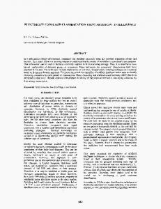
IEEE--ICET 2006 2nd International Conference on Emerging Technologies Peshawar, Pakistan, 13-14 November 2006
Hyperspectral Colon Tissue Classification using Morphological Analysis K Masood1, N Rajpoot 1, K Rajpoot2 and H Qureshi1 1
Department of Computer Science, University of Warwick, Coventry CV4 7AL, UK 2 GIK Institute of Engineering Sciences and Technology, Topi, Pakistan
Abstract. Diagnosis and cure of colon cancer can be improved by efficiently classifying the colon tissue cells into normal and malignant classes. This paper presents the classification of hyperspectral colon tissue cells using morphological analysis of gland nuclei cells. The application of hyperspectral imaging technique in medical image analysis is a new domain for researchers. The main advantage in using hyperspectral imaging is the increased spectral resolution and detailed subpixel information. Biopsy slides with several microdots, where each microdot is from a distinct patient, are illuminated with a tuned light source and magnification is performed upto 400X. The proposed classification algorithm combines the hyperspectral imaging technique with linear discriminant analysis. Dimensionality reduction and cellular segmentation is achieved by Independent Component Analysis (ICA) and k-means clustering. Morphological features, which describe the shape, orientation and other geometrical attributes, are next to be extracted. For classification, LDA is employed to discriminate tissue cells into normal and malignant classes. Implementation of LDA is simpler than other approaches; it saves the computational cost, while maintaining the performance. The algorithm is tested on a number of samples and its applicability is demonstrated with the help of measures such as classification accuracy rate and the area under the convex hull of ROC curves.
1 INTRODUCTION Colon cancer is a malignant disease of the large bowel. After lung and breast cancer, colorectal cancer (a combined term for colon and rectal cancer) is the most common cause of death for cancers in the Western world. The incidence of disease in England and Wales is about 30,000 cases/year, resulting in approximately 17,000 death/annum [14], and it has been estimated that at least half a million cases of colorectal cancer occur each year worldwide. It is caused by colonic polyps, an abnormal growth of tissue that projects in due course from the lining of the intestine or rectum, into colorectal cancer. These polyps are often benign and usually produce no symptoms. They may, however, cause painless rectal bleeding usually not apparent to the naked 1-4244-0502-5/06/$20.00©2006 IEEE
eye. The normal time for a polyp to reach 1 cm in diameter is five years or a little more. This 1 cm polyp will take around 5-10 years for the cancer to cause symptoms by which time it is frequently too late [13]. Diets low in fruits, less protein from vegetable sources, high age and family history are associated with increased risk of polyps. Persons smoking more than 20 cigarettes a day are 250 percent more likely to have polyps as opposed to nonsmokers who otherwise have the same risks. There is an association of cancer risk with meat, fat or protein consumption which appear to break down in the gut into cancer causing compounds called carcinogens [10]. Smoking cessation is important to decrease the likelihood of developing colon cancer. Dietary supplementation with 1500 mg of calcium or more a day is associated with a lower incidence of colon cancer. Weight reduction may be helpful in reducing the risk for colorectal cancer. Daily exercise reduces the likelihood of developing colon cancer. Turmeric, the spice which gives curry its distinctive yellow color, may also prevent colon cancer [7].
1.1 Hyperspectral Imaging Hyperspectral imaging in laboratory experiments, is a non-contact sensing technique for obtaining both spectral and spatial information about a tissue sample. Hyperspectral imaging measures a spectrum for each pixel in an image. There are many types of spectroscopy which are being used to study the spectral signatures of individual cells and underlying tissue sections. In optical spectroscopy, which measures transmission through, or reflectance from, a sample by visible or near-infrared radiation at the same wavelength as the source, classification is done mostly by statistical measures [1]. Hyperspectral images are normally produced by
735
signatures present in an optical field during a single-pass evaluation, including molecules with overlapping but distinct emission spectra. High resolution characteristics of hyperspectal imaging is reflected in two sample images in Figure 1 of colon tissue cells.
emission of spectra from imaging spectrometers. Spectroscopy is the study of light that is emitted by or reflected from materials and its variation in energy with wavelength [12]. Spectrometers are used to make measurements of the light reflected from a test specimen. A prism in the center of spectrometer splits this light into many different wavelength bands and the energy in each band is measured by detectors which are different for each band. By using large number of detectors (even a few thousand), spectrometers can make spectral measurements of bands as narrow as 0.01 micrometers over a wide wavelength range, typically at least 0.4 to 2.4 micrometers (visible through middle infrared wavelength ranges). Most approaches to analyse hyperspectral images concentrate on the spectral information in individual image cells, rather than spatial variations within individual bands or groups of bands. The statistical classification (clustering) methods often used with multispectral images can also be applied to hyperspectral images but may need to be adapted to handle high dimensionality.
2 Dimensionality Reduction and Subspace Projection
There is a large redundant information in the subbands of hyperspectral imagery. Independent component analysis (ICA) is used to discard the redundancy and extract the variance among different wavelengths of spectra. K-means clustering is used to help the dimensionality reduction procedure and to segregate the biopsy slide into its cellular components. Subspace projection is achieved with principal component analysis (PCA) and linear discriminant analysis (LDA). A brief introduction to the mathematical derivation of these methods is presented in the following subsections.
2.1 Independent Component Analysis (ICA)
Recent developments in hyperspectral imaging have enhanced the usefulness of the light microscope [4]. A standard epifluorescence microscope can be optically coupled to an imaging spectrograph, with output recorded by a CCD camera. Individual images are captured representing Y-wavelength planes, with the stage successively moved in the X direction, allowing an image cube to be constructed from the compilation of generated scan files. Hyperspectral imaging microscopy permits the capture and identification of different spectral
The objective of Independent Component Analysis (ICA) is to perform a dimension reduction approach to achieve decorrelation between independent components [16]. Let us denote by X = (x1, x2, . . . , xm )T a zero-mean mdimensional variable, and S = (s1 ,s2, …,sn )T , n < m, is its linear transform with a constant matrix W [17]: S = WX
Given X as observations, ICA aims to estimating
(a) Normal cells
(b) Malignant cells Figure 1. Segmentation Results
736
2.3 Linear Discriminant Analysis
W and S. The goal of ICA is to find a new variable S such that transformed components si are not only uncorrelated with each other, but also statistically as independent of each other as possible. An ICA algorithm consists of two parts, an objective function which measures the independence between components, entropy of each independent source or their higher order cumulants, and the second part is the optimisation method used to optimise the objective function. Higher order cumulants like kurtosis, and approximations of negentropy provide one-unit objective function. A decorrelation method is needed to prevent the objective function from converging to the same optimum for different independent components. Whitening or data sphering project the data onto its subspace as well as normalizing its variance.
LDA is closely related to principal component analysis (PCA) and factor analysis in that both look for linear combinations of variables which best explain the data. LDA explicitly attempts to model the difference between the classes of data. PCA on the other hand does not take into account any difference in class, and factor analysis builds the feature combinations based on differences rather than similarities. Discriminant analysis is also different from factor analysis in that it is not an interdependence technique : a distinction between independent variables and dependent variables (also called criterion variables) must be made. The LDA method is proposed to take into consideration global as well as local variation of training images. It uses both principal component analysis and linear discriminant analysis to produce a subspace projection matrix. The advantage is in using within-class information, minimizing variation within each class and maximizing between class variation, thus obtaining more discriminant information from the data. Three scatter matrices, representing the within-class (Sw ), between-class (Sb ) and total scatter (St ), are computed for the training data set.
2.2 K-Means Clustering Clustering is the process of partitioning or grouping a given set of patterns into disjoint clusters. This is done such that patterns in the same cluster are alike and patterns belonging to two different clusters are different. The k-means method has been shown to be effective in producing good clustering results for many practical applications [2]. The aim of the kmeans algorithm is to divide m points in n dimensions into k clusters so that the withincluster sum of squared distance from the cluster centroids is minimised. The algorithm requires as input a matrix of m points in n dimensions and a matrix of k initial cluster centres in n dimensions. The number of clusters k is assumed to be fixed in k-means clustering. Let the k prototypes (w1 , . . . , wk ) be initialised to one of the m input patterns (i1 , . . . , im ). Therefore;
¦¦ i � w 1
j 1 i1 IC ˆ
T
C
¦ Ni �Yi � Y �Yi � Y
Sb
i 1
T
C
¦ � Gk � Yi � Gk � Yi
SW
i 1
The appropriate choice of k is problem and domain dependent and generally a user must try several values of k. The quality of the clustering is determined by the following error function:
E
¦ � Gn � Y � Gn � Y n 1
wj = il , j Î {1, . . . , k}, l Î {1, . . . , m}
k
T
M
St
where Y vector
Yi
2 j
1 Xi
1 M
M
¦G
n
is the average feature
n 1
of
the
¦G
i
ˆ iIX i
G
training
set
and
is the average feature
vector of the ith individual class.
j
LDA algorithm takes advantage of the fact that, under some idealized conditions, the variation
The direct implementation of k-means method is computationally very intensive.
737
SEGMENTATION
Input Hyperspectral Image Data Cubes
FEATURE EXTRACTION Segmented Label Image
Data Cubes (Reduced Dimensions)
ICA
Computation of Morphological Features
k-means Clustering
CLASSIFICATION Subspace Projected Feature Vectors Match
PCA Analysis
Feature Vectors
Recognition (Euclidian distance) LDA Analysis
Figure 2 Classification Algorithm Block Diagram
3.1 Segmentation
within class lies in a linear subspace of the image space. Hence, the classes are convex, and, therefore linearly separable. LDA is a class specific method, in the sense that it tries to ’shape’ the scatter in order to make it more reliable for classification. It is clear that, although PCA achieves larger total scatter, LDA achieves greater between-class scatter, and consequently, yield improved classification [3].
High dimensional data in the form of cubes is obtained using hyperspectral imaging. For efficient processing this data has to be dimensionally reduced. Dimensionality reduction involves two steps, extraction of statistically independent components using Independent Component Analysis (ICA) and colour segmentation using k-means clustering. Flexible ICA (FlexICA) [8], a fixed point algorithm for ICA, adopting a generalised Gaussian density, is used for data sphering (whitening) and achieves considerable dimensionality reduction. Data is distributed towards heavy-tailedness by the high-emphasis filters. The data with reduced dimensionality is then fed to k-means clustering algorithm for segmentation.
3. METHODOLOGY The proposed classification algorithm consists of three modules as shown in Figure 2. Brief description of dimensionality reduction and feature extraction modules is given in the following sub-sections. Detailed description of the segmentation can be found in [15].
(a) Benign cells
(b) Malignant cells
Figure 3 Segmentation Results
738
Table 1 Classification Results Single Single Multi Single Single Single Single Single Single Single Multi
Patch 16x16 16x16 16x16,32x32,.. 16x16 16x16 16x16 16x16 32x32 32x32 32x32 16x16,32x32,..
Features 1 (Euler No.) 2 (ENo,CA) 5 (ENo,CA,A,E,O) 2 (ENo,CA) 3 (ENo,CA,A) 5 (ENo,CA,A,E,O) 10 (5+5 Elliptical) 2 (ENo,CA) 5 (ENo,CA,A,E,O) 10 (5+5 ELliptical) 5 (ENo,CA,A,E,O)
Method PCA PCA PCA LDA LDA LDA LDA LDA LDA LDA LDA
Accuracy (%) 51 51.4 75 55.5 55.7 56.4 56.4 60.1 61.3 61.3 84
cellular components. In each binary image, the corresponding cellular components i.e. nuclei, cytoplasm, gland secretions and stroma of lamina propria have binary value equal to 1.
The hyperspectal data cube containing 28 subbands is segmented into four labeled parts. Each slide of the tissue cells is divided into four regions represented by four colours as shown in Figure 3. The four labeled parts are denoted by colours as dark blue for nuclei, light blue for cytoplasm, yellow for gland secretions and red for lamina propria.
4. EXPERIMENTS 4.1 Experimental Setup The experimental setup consists of a unique tuned light source based on a digital mirror device (DMD), a Nikon Biophot microscope and a CCD camera. Two different biopsy slides containing several microdots, where each microdot is from a distinct patient, is prepared. Then each slide is illuminated with a tuned light source (capable of emitting any combination of light frequencies in the range of 450-850 nm), followed by magnification to 400 X. Thus several images, each image using a different combination of light frequencies, are produced [5].
3.2Feature Extraction In order for the pattern recognition process to be tractable it is necessary to represent patterns into some mathematical or analytical model. The model should convert patterns into features or measurable values, which are condensed representations of the patterns, containing only salient information [9]. Features contain the characteristics of a pattern to make them comparable to standard templates making the pattern classification possible. The extraction of good features from these pattern models and the selection from them of the ones with the most discriminatory power are the basis for the success of the classification process. In this work morphological texture features, extracted from the segmented images of a hyperspectral data cube for a biopsy slide of colon tissue cells, are used for the classification of the tissue cells.
Hyperspectral image data cubes, equivalent to the number of input biopsy slides, are produced using hyperspectral analysis for twenty eight subbands of light. The dimension of each cube is 1024 × 1024 × 28. Performing FlexICA and kmeans clustering for segmentation, we get images having 1024 × 1024 dimensions per slide. For single scale experiments, each image is divided into 4096 patches of 16 × 16 dimensions per patch. Morphological operation is performed on the patches for extraction of feature vectors using different combinations of ten scalar morphological properties. Two sets of
Morphological features, which describe the shape, size, orientation and other geometrical attributes of the cellular components, are extracted to discriminate between two classes of input data. The segmented image is first split into four binarised image in accordance with the four
739
(a) ROC
(b) AUCH Figure 4. ROC & AUCH Performance Curves
ideal AUCH curve (top left hand corner), resulting with better classification rate. The AUCH for LDA is larger than AUCH for PCA which shows better performance of LDA as compared to PCA.
experiments are carried, one for PCA and other for LDA. The data (patches of all slides randomly mixed) is divided into training set (about one quarter of the patches) and test set (remaining three quarters of patches).
4.2 Results
5. CONCLUSIONS
Selecting only a few eigenvectors and performing PCA, classification rate of 75 percent is achieved. LDA is performed in a modular form [6] in which each slide of image represents a separate class. Thus two classes of benign and malignant cells are divided into eleven subclasses and taking eigenvectors with large eigenvalues, we get on the average 84 percent classification rate. The results are encouraging in terms of the computation speed and ease of implementation. The accuracy in the table refers to the percentage of correctly classified patches.
In this paper, classification of colon tissue cells is achieved using the morphology of the glandular cells of the tissue region. There is an indication that the morphology of the cells, obtained from the hyperspectral analysis of biopsy slides, has enough discriminatory power to apply a simple classifier for its efficient classification. Regular structured cell shapes with some orientations are characteristics of normal cells, whereas irregular and deformed cell shapes represent malignant tissue. Segmentation and dimensionality reduction is performed using k-means clustering and independent component analysis. Single scale and multiscale feature extraction is employed. Single scale features depend on the patch size and with increase in patch size classification accuracy increases, but with a reduced spatial resolution for classification. Multiscale feature extraction produces a bias in the testing mechanism, as test patches carry some common global information from the training patches.
The ROC curves along with the AUCH (Area under convex hull) are shown in Figure 4. ROC curve shows the performance of a particular classifier in terms of true positive and false positive rates [11]. ROC curve gives the optimum threshold which is defined in terms of Euclidean distance of each test patch with all training patches. At the starting point, there are some True Positives but there are no False Positives. As threshold increases, there is increase in positive alarms but simultaneously false positives begin to rise. When threshold becomes maximum than every case is claimed positive and it represents top right hand corner. Area under convex hull (AUCH) shows the performance of classifier with the increase in the number of discriminant features. As the area under the curve increases, it will approximate to
ACKNOWLEDGMENTS The authors are greatly indebted to Gustave Davis, Mauro Maggioni and Ronald Coifman of the School of Medicine and the Applied Mathematics Department of Yale University for providing the data and for many fruitful discussions.
740
REFERENCES
9.
1. John Adams, M. Smith, and A. Gillespie. Imaging spectroscopy: Interpretation based on spectral mixture analysis. Remote Geochemical Analysis, 1993.
Anil Jain, Robert Duin, and Jianchang Mao. Statistical pattern recognition: A review. IEEE Trans. on Pattern Analysis and Machine Intelligence, 22, 2000.
10.
S. Kaster, S. Buckley, and T. Haseman. Colonoscopy and barium enema in the detection of colorectal cancer. Gastrointestinal Endoscopy, 1995.
2. K. Alsabti, S. Ranka, and V. Singh. An efficient kmeans clustering algorithm. www.cise.ufl.edu., 1997. 3.
Belhumeur, J. Hesponha, and D. Kriegman. Eigenfaces vs fisherfaces: Recognition using class specific linear projection. IEEE Trans.Pattern Analysis and Machine Intelligence, 1997.
4.
E. A. Cloutis. Hyperspectral geological remote sensing. Evaluation of Analytical TechniquesInternational Journal of Remote Sensing, 17:22152242, 1996.
11. A. Khan, A. Majid, and A. Mirza. Combination and optimization of classifier in gender classification using genetic program ming. International Journal of Knowledge Based and Intelligent Engineering Systems, 9:1-11, 2005. 12.
13. D. E. Mansell. Colon polyps & colon cancer. American Cancer Society Textbook of Clinical Oncology, 1991.
5. G. Davis, M. Maggioni, and R. Coifman et al. Spectral/spatial analysis of colon carcinoma. Journal of Modern Pathology, 2003.
14. Office of National Statistics. Cancer statistics: Registrations, england and wales. london. HMSO, 1999.
6. R. Gottmukul and V. K. Asari. An improved face recognition technique based on modular pca approach. Pattern Recognition Letters, 25:429436, 2004. 7.
David Landgrebe. Hyperspectral image data analysis as a high dimensional signal processing problem. IEEE Signal Processing magazine, 2002.
15.
K. M. Rajpoot and Nasir M Rajpoot. Hyperspectral colon tissue cell classification. SPIE Medical Imaging (MI), 2004.
16.
Kun Zhang and Lai-Wan Chan. Dimension reduction based on orthogonality-a decorrelation method in ica. ICANN/ICONIP, 2003.
R. S. Houlston. Molecular pathology of of colorectal cancer. Clinical Pathology, 2001.
8. A. Hyvarinen. Survey on independent component analysis. Neural Computing Surveys, 2:94-128, 1999.
741