Hypothesis Testing Using z- and t-tests In hypothesis testing, one ...

B. Weaver (27-May-2011)

z- and t-tests ... 1

Hypothesis Testing Using z- and t-tests In hypothesis testing, one attempts to answer the following question: If the null hypothesis is assumed to be true, what is the probability of obtaining the observed result, or any more extreme result that is favourable to the alternative hypothesis?1 In order to tackle this question, at least in the context of z- and t-tests, one must first understand two important concepts: 1) sampling distributions of statistics, and 2) the central limit theorem. Sampling Distributions Imagine drawing (with replacement) all possible samples of size n from a population, and for each sample, calculating a statistic--e.g., the sample mean. The frequency distribution of those sample means would be the sampling distribution of the mean (for samples of size n drawn from that particular population). Normally, one thinks of sampling from relatively large populations. But the concept of a sampling distribution can be illustrated with a small population. Suppose, for example, that our population consisted of the following 5 scores: 2, 3, 4, 5, and 6. The population mean = 4, and the population standard deviation (dividing by N) = 1.414. If we drew (with replacement) all possible samples of 2 from this population, we would end up with the 25 samples shown in Table 1. Table 1: All possible samples of n=2 from a population of 5 scores. Sample # 1 2 3 4 5 6 7 8 9 10 11 12 13

First Score 2 2 2 2 2 3 3 3 3 3 4 4 4

Second Score 2 3 4 5 6 2 3 4 5 6 2 3 4

Sample Mean 2 2.5 3 3.5 4 2.5 3 3.5 4 4.5 3 3.5 4

Sample # 14 15 16 17 18 19 20 21 22 23 24 25

First Score 4 4 5 5 5 5 5 6 6 6 6 6

Second Score 5 6 2 3 4 5 6 2 3 4 5 6

Mean of the sample means = SD of the sample means =

Sample Mean 4.5 5 3.5 4 4.5 5 5.5 4 4.5 5 5.5 6 4.000 1.000

(SD calculated with division by N)

1

That probability is called a p-value. It is a really a conditional probability--it is conditional on the null hypothesis being true.



The 25 sample means from Table 1 are plotted below in Figure 1 (a histogram). This distribution of sample means is called the sampling distribution of the mean for samples of n=2 from the population of interest (i.e., our population of 5 scores).

Distribution of Sample Means* 6

5

4

3

2 Std. Dev = 1.02

1

Mean = 4.00 N = 25.00

0 2.00

2.50

3.00

3.50

4.00

4.50

5.00

5.50

6.00

MEANS * or "Sampling Distribution of the Mean"

Figure 1: Sampling distribution of the mean for samples of n=2 from a population of N=5.

I suspect the first thing you noticed about this figure is peaked in the middle, and symmetrical about the mean. This is an important characteristic of sampling distributions, and we will return to it in a moment. You may have also noticed that the standard deviation reported in the figure legend is 1.02, whereas I reported SD = 1.000 in Table 1. Why the discrepancy? Because I used the population SD formula (with division by N) to compute SD = 1.000 in Table 1, but SPSS used the sample SD formula (with division by n-1) when computing the SD it plotted alongside the histogram. The population SD is the correct one to use in this case, because I have the entire population of 25 samples in hand. The Central Limit Theorem (CLT) If I were a mathematical statistician, I would now proceed to work through derivations, proving the following statements:



1. The mean of the sampling distribution of the mean = the population mean 2. The SD of the sampling distribution of the mean = the standard error (SE) of the mean = the population standard deviation divided by the square root of the sample size Putting these statements into symbols:

µ X = µ X { mean of the sample means = the population mean }

σX =

σX n

{ SE of mean = population SD over square root of n }

(1.1)

(1.2)

But alas, I am not a mathematical statistician. Therefore, I will content myself with telling you that these statements are true (those of you who do not trust me, or are simply curious, may consult a mathematical stats textbook), and pointing to the example we started this chapter with. For that population of 5 scores, µ = 4 and σ = 1.414 . As shown in Table 1, µ X = µ = 4 , and σ X = 1.000 . According to equation (1.2), if we divide the population SD by the square root of the sample size, we should obtain the standard error of the mean. So let's give it a try:

σ n

=

1.414 2

= .9998 1

(1.3)

When I performed the calculation in Excel and did not round off σ to 3 decimals, the solution worked out to 1 exactly. In the Excel worksheet that demonstrates this, you may also change the values of the 5 population scores, and should observe that σ X = σ n for any set of 5 scores you choose. Of course, these demonstrations do not prove the CLT (see the aforementioned mathstats books if you want proof), but they should reassure you that it does indeed work. What the CLT tells us about the shape of the sampling distribution

The central limit theorem also provides us with some very helpful information about the shape of the sampling distribution of the mean. Specifically, it tells us the conditions under which the sampling distribution of the mean is normally distributed, or at least approximately normal, where approximately means close enough to treat as normal for practical purposes. The shape of the sampling distribution depends on two factors: the shape of the population from which you sampled, and sample size. I find it useful to think about the two extremes: 1. If the population from which you sample is itself normally distributed, then the sampling distribution of the mean will be normal, regardless of sample size. Even for sample size = 1, the sampling distribution of the mean will be normal, because it will be an exact copy of the population distribution.



2. If the population from which you sample is extremely non-normal, the sampling distribution of the mean will still be approximately normal given a large enough sample size (e.g., some authors suggest for sample sizes of 300 or greater). So, the general principle is that the more the population shape departs from normal, the greater the sample size must be to ensure that the sampling distribution of the mean is approximately normal. This tradeoff is illustrated in the following figure, which uses colour to represent the shape of the sampling distribution (purple = non-normal, red = normal, with the other colours representing points in between).

Does n have to be ≥ 30?

Some textbooks say that one should have a sample size of at least 30 to ensure that the sampling distribution of the mean is approximately normal. The example we started with (i.e., samples of n = 2 from a population of 5 scores) suggests that this is not correct (see Figure 1). Here is another example that makes the same point. The figure on the left, which shows the age distribution for all students admitted to the Northern Ontario School of Medicine in its first 3 years of operation, is treated as the population. The figure on the right shows the distribution of means for 10,000 samples of size 16 drawn from that population. Notice that despite the severe



positive skew in the population, the distribution of sample means is near enough to normal for the normal approximation to be useful.

What is the rule of 30 about then?

In the olden days, textbook authors often did make a distinction between small-sample and largesample versions of t-tests. The small- and large-sample versions did not differ at all in terms of how t was calculated. Rather, they differed in how/where one obtained the critical value to which they compared their computed t-value. For the small-sample test, one used the critical value of t, from a table of critical t-values. For the large-sample test, one used the critical value of z, obtained from a table of the standard normal distribution. The dividing line between small and large samples was usually n = 30 (or sometimes 20). Why was this done? Remember that in that era, data analysts did not have access to desktop computers and statistics packages that computed exact p-values. Therefore, they had to compute the test statistic, and compare it to the critical value, which they looked up in a table. Tables of critical values can take up a lot of room. So when possible, compromises were made. In this particular case, most authors and statisticians agreed that for n ≥ 30, the critical value of z (from the standard normal distribution) was close enough to the critical value of t that it could be used as an approximation. The following figure illustrates this by plotting critical values of t with



alpha = .05 (2-tailed) as a function of sample size. Notice that when n ≥ 30 (or even 20), the critical values of t are very close to 1.96, the critical value of z.

Nowadays, we typically use statistical software to perform t-tests, and so we get a p-value computed using the appropriate t-distribution, regardless of the sample size. Therefore the distinction between small- and large-sample t-tests is no longer relevant, and has disappeared from most modern textbooks. The sampling distribution of the mean and z-scores

When you first encountered z-scores, you were undoubtedly using them in the context of a raw score distribution. In that case, you calculated the z-score corresponding to some value of X as follows: z=

X −µ

σ

=

X − µX

σX

(1.4)

And, if the distribution of X was normal, or at least approximately normal, you could then take that z-score, and refer it to a table of the standard normal distribution to figure out the proportion of scores higher than X, or lower than X, etc. Because of what we learned from the central limit theorem, we are now in a position to compute a z-score as follows:



z=

X − µX

σX

=

X −µ

σ

(1.5)

n

This is the same formula, but with X in place of X, and σ X in place of σ X . And, if the sampling distribution of X is normal, or at least approximately normal, we may then refer this value of z to the standard normal distribution, just as we did when we were using raw scores. (This is where the CLT comes in, because it tells the conditions under which the sampling distribution of X is approximately normal.) An example. Here is a (fictitious) newspaper advertisement for a program designed to increase intelligence of school children2:

As an expert on IQ, you know that in the general population of children, the mean IQ = 100, and the population SD = 15 (for the WISC, at least). You also know that IQ is (approximately) normally distributed in the population. Equipped with this information, you can now address questions such as: If the n=25 children from Dundas are a random sample from the general population of children, a) What is the probability of getting a sample mean of 108 or higher? b) What is the probability of getting a sample mean of 92 or lower? c) How high would the sample mean have to be for you to say that the probability of getting a mean that high (or higher) was 0.05 (or 5%)? d) How low would the sample mean have to be for you to say that the probability of getting a mean that low (or lower) was 0.05 (or 5%)?

2

I cannot find the original source for this example, but I believe I got it from Dr. Geoff Norman, McMaster University.



The solutions to these questions are quite straightforward, given everything we have learned so far in this chapter. If we have sampled from the general population of children, as we are assuming, then the population from which we have sampled is at least approximately normal. Therefore, the sampling distribution of the mean will be normal, regardless of sample size. Therefore, we can compute a z-score, and refer it to the table of the standard normal distribution. So, for part (a) above: z=

X − µX

σX

=

X − µX

σX

=

n

108 − 100 8 = = 2.667 15 3 25

(1.6)

And from a table of the standard normal distribution (or using a computer program, as I did), we can see that the probability of a z-score greater than or equal to 2.667 = 0.0038. Translating that back to the original units, we could say that the probability of getting a sample mean of 108 (or greater) is .0038 (assuming that the 25 children are a random sample from the general population). For part (b), do the same, but replace 108 with 92:

z=

X − µX

σX

=

X − µX

σX

=

n

92 − 100 −8 = = −2.667 15 3 25

(1.7)

Because the standard normal distribution is symmetrical about 0, the probability of a z-score equal to or less than -2.667 is the same as the probability of a z-score equal to or greater than 2.667. So, the probability of a sample mean less than or equal to 92 is also equal to 0.0038. Had we asked for the probability of a sample mean that is either 108 or greater, or 92 or less, the answer would be 0.0038 + 0.0038 = 0.0076. Part (c) above amounts to the same thing as asking, "What sample mean corresponds to a z-score of 1.645?", because we know that p ( z ≥ 1.645) = 0.05 . We can start out with the usual z-score formula, but need to rearrange the terms a bit, because we know that z = 1.645, and are trying to determine the corresponding value of X . z=

X − µX

σX

{ cross-multiply to get to next line }

zσ X = X − µ X { add µ X to both sides } (1.8) zσ X + µ X = X { switch sides }

(

X = zσ X + µ X = 1.645 15

)

25 + 100 = 104.935



So, had we obtained a sample mean of 105, we could have concluded that the probability of a mean that high or higher was .05 (or 5%). For part (d), because of the symmetry of the standard normal distribution about 0, we would use the same method, but substituting -1.645 for 1.645. This would yield an answer of 100 - 4.935 = 95.065. So the probability of a sample mean less than or equal to 95 is also 5%. The single sample z-test

It is now time to translate what we have just been doing into the formal terminology of hypothesis testing. In hypothesis testing, one has two hypotheses: The null hypothesis, and the alternative hypothesis. These two hypotheses are mutually exclusive and exhaustive. In other words, they cannot share any outcomes in common, but together must account for all possible outcomes. In informal terms, the null hypothesis typically states something along the lines of, "there is no treatment effect", or "there is no difference between the groups".3 The alternative hypothesis typically states that there is a treatment effect, or that there is a difference between the groups. Furthermore, an alternative hypothesis may be directional or non-directional. That is, it may or may not specify the direction of the difference between the groups. H 0 and H1 are the symbols used to represent the null and alternative hypotheses respectively. (Some books may use H a for the alternative hypothesis.) Let us consider various pairs of null and alternative hypotheses for the IQ example we have been considering. Version 1: A directional alternative hypothesis H 0 : µ ≤ 100 H1 : µ > 100 This pair of hypotheses can be summarized as follows. If the alternative hypothesis is true, the sample of 25 children we have drawn is from a population with mean IQ greater than 100. But if the null hypothesis is true, the sample is from a population with mean IQ equal to or less than 100. Thus, we would only be in a position to reject the null hypothesis if the sample mean is greater than 100 by a sufficient amount. If the sample mean is less than 100, no matter by how much, we would not be able to reject H 0 . How much greater than 100 must the sample mean be for us to be comfortable in rejecting the null hypothesis? There is no unequivocal answer to that question. But the answer that most 3

I said it typically states this, because there may be cases where the null hypothesis specifies a difference between groups of a certain size rather than no difference between groups. In such a case, obtaining a mean difference of zero may actually allow you to reject the null hypothesis.



disciplines use by convention is this: The difference between X and µ must be large enough that the probability it occurred by chance (given a true null hypothesis) is 5% or less. The observed sample mean for this example was 108. As we saw earlier, this corresponds to a zscore of 2.667, and p( z ≥ 2.667) = 0.0038 . Therefore, we could reject H 0 , and we would act as if the sample was drawn from a population in which mean IQ is greater than 100. Version 2: Another directional alternative hypothesis H 0 : µ ≥ 100 H1 : µ < 100 This pair of hypotheses would be used if we expected the Dr. Duntz's program to lower IQ, and if we were willing to include an increase in IQ (no matter how large) under the null hypothesis. Given a sample mean of 108, we could stop without calculating z, because the difference is in the wrong direction. That is, to have any hope of rejecting H 0 , the observed difference must be in the direction specified by H1 . Version 3: A non-directional alternative hypothesis H 0 : µ = 100 H1 : µ ≠ 100 In this case, the null hypothesis states that the 25 children are a random sample from a population with mean IQ = 100, and the alternative hypothesis says they are not--but it does not specify the direction of the difference from 100. In the first directional test, we needed to have X > 100 by a sufficient amount, and in the second directional test, X < 100 by a sufficient amount in order to reject H 0 . But in this case, with a non-directional alternative hypothesis, we may reject H 0 if

X < 100 or if X > 100 , provided the difference is large enough. Because differences in either direction can lead to rejection of H 0 , we must consider both tails of the standard normal distribution when calculating the p-value--i.e., the probability of the observed outcome, or a more extreme outcome favourable to H1 . For symmetrical distributions like the standard normal, this boils down to taking the p-value for a directional (or 1-tailed) test, and doubling it. For this example, the sample mean = 108. This represents a difference of +8 from the population mean (under a true null hypothesis). Because we are interested in both tails of the distribution, we must figure out the probability of a difference of +8 or greater, or a change of -8 or greater. In other words, p = p( X ≥ 108) + p( X ≤ 92) = .0038 + .0038 = .0076 .



Single sample t-test (when σ is not known)

In many real-world cases of hypothesis testing, one does not know the standard deviation of the population. In such cases, it must be estimated using the sample standard deviation. That is, s (calculated with division by n-1) is used to estimate σ . Other than that, the calculations are as we saw for the z-test for a single sample--but the test statistic is called t, not z.

t( df = n −1) =

X − µX sX

where s X =

s n

, and s =

∑( X − X ) n −1

2

=

SS X n −1

(1.9)

In equation (1.9), notice the subscript written by the t. It says "df = n-1". The "df" stands for degrees of freedom. "Degrees of freedom" can be a bit tricky to grasp, but let's see if we can make it clear. Degrees of Freedom Suppose I tell you that I have a sample of n=4 scores, and that the first three scores are 2, 3, and 5. What is the value of the 4th score? You can't tell me, given only that n = 4. It could be anything. In other words, all of the scores, including the last one, are free to vary: df = n for a sample mean. To calculate t, you must first calculate the sample standard deviation. The conceptual formula for the sample standard deviation is:

s=

∑( X − X )

2

n −1

(1.10)

Suppose that the last score in my sample of 4 scores is a 6. That would make the sample mean equal to (2+3+5+6)/4 = 4. As shown in Table 2, the deviation scores for the first 3 scores are -2, -1, and 1. Table 2: Illustration of degrees of freedom for sample standard deviation Score 2 3 5 --

Mean 4 4 4 --

Deviation from Mean -2 -1 1 x4



Using only the information shown in the final column of Table 2, you can deduce that x4 , the 4th deviation score, is equal to -2. How so? Because by definition, the sum of the deviations about the mean = 0. This is another way of saying that the mean is the exact balancing point of the distribution. In symbols:

∑( X − X ) = 0

(1.11)

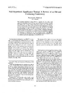
So, once you have n-1 of the ( X − X ) deviation scores, the final deviation score is determined. That is, the first n-1 deviation scores are free to vary, but the final one is not. There are n-1 degrees of freedom whenever you calculate a sample variance (or standard deviation). The sampling distribution of t To calculate the p-value for a single sample z-test, we used the standard normal distribution. For a single sample t-test, we must use a t-distribution with n-1 degrees of freedom. As this implies, there is a whole family of t-distributions, with degrees of freedom ranging from 1 to infinity ( ∞ = the symbol for infinity). All t-distributions are symmetrical about 0, like the standard normal. In fact, the t-distribution with df = ∞ is identical to the standard normal distribution. But as shown in Figure 2 below, t-distributions with df < infinity have lower peaks and thicker tails than the standard normal distribution. To use the technical term for this, they are leptokurtic. (The normal distribution is said to be mesokurtic.) As a result, the critical values of t are further from 0 than the corresponding critical values of z. Putting it another way, the absolute value of critical t is greater than the absolute value of critical z for all t-distributions with df < ∞ : For df < ∞,

tcritical > zcritical

(1.12)

Probability density functions .5

Standard Normal Distribution

.4

t-distribution with df = 10

.3

.2

t-distribution with df = 2

.1

0.0 -6

-4

-2

0

2

4

6



Figure 2: Probability density functions of: the standard normal distribution (the highest peak with the thinnest tails); the t-distribution with df=10 (intermediate peak and tails); and the t-distribution with df=2 (the lowest peak and thickest tails). The dotted lines are at -1.96 and +1.96, the critical values of z for a two-tailed test with alpha = .05. For all t-distributions with df < ∞ , the proportion of area beyond -1.96 and +1.96 is greater than .05. The lower the degrees of freedom, the thicker the tails, and the greater the proportion of area beyond -1.96 and +1.96.

Table 3 (see below) shows yet another way to think about the relationship between the standard normal distribution and various t-distributions. It shows the area in the two tails beyond -1.96 and +1.96, the critical values of z with 2-tailed alpha = .05. With df=1, roughly 15% of the area falls in each tail of the t-distribution. As df gets larger, the tail areas get smaller and smaller, until the t-distribution converges on the standard normal when df = infinity. Table 3: Area beyond critical values of + or -1.96 in various t-distributions. The t-distribution with df = infinity is identical to the standard normal distribution. Degrees of Freedom 1 2 3 4 5 10 15 20 25 30

Area beyond + or -1.96 0.30034 0.18906 0.14485 0.12155 0.10729 0.07844 0.06884 0.06408 0.06123 0.05934

Degrees of Freedom 40 50 100 200 300 400 500 1,000 5,000 10,000 Infinity

Area beyond + or -1.96 0.05699 0.05558 0.05278 0.05138 0.05092 0.05069 0.05055 0.05027 0.05005 0.05002 0.05000

Example of single-sample t-test. This example is taken from Understanding Statistics in the Behavioral Sciences (3rd Ed), by Robert R. Pagano. A researcher believes that in recent years women have been getting taller. She knows that 10 years ago the average height of young adult women living in her city was 63 inches. The standard deviation is unknown. She randomly samples eight young adult women currently residing in her city and measures their heights. The following data are obtained: [64, 66, 68, 60, 62, 65, 66, 63.]

The null hypothesis is that these 8 women are a random sample from a population in which the mean height is 63 inches. The non-directional alternative states that the women are a random sample from a population in which the mean is not 63 inches.



H 0 : µ = 63 H1 : µ ≠ 63 The sample mean is 64.25. Because the population standard deviation is not known, we must estimate it using the sample standard deviation.

∑(X − X )

sample SD = s =

2

n −1

(1.13) =

(64 − 64.25) 2 + (66 − 64.25) 2 + ...(63 − 64.25) 2 = 2.5495 7

We can now use the sample standard deviation to estimate the standard error of the mean: Estimated SE of mean = s X =

s n

=

2.5495 8

= 0.901

(1.14)

And finally:

t=

X − µ0 64.25 − 63 = = 1.387 0.901 sX

(1.15)

This value of t can be referred to a t-distribution with df = n-1 = 7. Doing so, we find that the conditional probability4 of obtaining a t-statistic with absolute value equal to or greater than 1.387 = 0.208. Therefore, assuming that alpha had been set at the usual .05 level, the researcher cannot reject the null hypothesis. I performed the same test in SPSS (AnalyzeÆCompare MeansÆOne sample t-test), and obtained the same results, as shown below. T-TEST /TESTVAL=63 /*