Identification and Likelihood Inference for Recursive ... - CiteSeerX

Identification and Likelihood Inference for Recursive Linear Models with Correlated Errors Mathias Drton Department of Statistics The University of Chicago Chicago, IL 60637

Michael Eichler Institut f¨ ur Angewandte Mathematik Universität Heidelberg Im Neuenheimer Feld 294 69120 Heidelberg, Germany

Thomas S. Richardson Department of Statistics University of Washington Seattle, WA 98195-4322

Working Paper no. 59 Center for Statistics and the Social Sciences University of Washington 12 Aug 2006

Abstract In recursive linear models, the multivariate normal joint distribution of all variables exhibits a dependence structure induced by recursive systems of linear structural equations. Such models appear in particular in seemingly unrelated regressions, structural equation modelling, simultaneous equation systems, and in Gaussian graphical modelling. We show that recursive linear models that are ‘bow-free’ are well-behaved statistical models, namely, they are everywhere identifiable and form curved exponential families. Here, ‘bow-free’ refers to models satisfying the condition that if a variable x occurs in the structural equation for y, then the errors for x and y are uncorrelated. For the computation of maximum likelihood estimates in ‘bow-free’ recursive linear models we introduce the Residual Iterative Conditional Fitting (RICF) algorithm. Compared to existing algorithms RICF is easily implemented requiring only least squares computations, has clear convergence properties, and finds parameter estimates in closed form whenever possible. KEY WORDS: Linear structural equation model; curved exponential family; maximum likelihood estimation; residual iterative conditional fitting; bow-free acyclic path diagrams; BAP.

1

Introduction

A system of linear structural equations determines a dependence pattern among a fixed set of variables by dictating that, up to a random error term, each variable is equal to a linear combination of some of the remaining variables. Traditionally the error terms are assumed to follow a joint multivariate normal distribution with mean vector equal to zero. Thus a system of linear structural equations induces a multivariate linear model for the variables under consideration. Presenting a formalism for simultaneously representing causal and statistical hypotheses relating a set of variables, these multivariate linear models are widely used in the social sciences and elsewhere, where they are often called structural equation models. Several hundred papers make use of the methodology; for some examples see Bollen [6]. In seminal work, Wright [71, 72, 73] introduced path diagrams, which are very useful graphical representations of structural equations. A path diagram consists of a graph with one vertex for each variable, and containing directed and bi-directed edges. A directed edge i → j indicates that variable i appears in the equation for variable j. Thus the directed edges in a path diagram are in correspondence with the path coefficients, that is, the coefficients appearing in the linear structural equations. A bidirected edge i ↔ j indicates correlation between the errors in the equations for variables i and j. (For a formal definition of path diagrams see §2.2.)

1.1

Challenges in structural equation modelling

Since their inception structural equation models and path diagrams have often been the subject of suspicion and controversy; see e.g. Niles [42]. The resulting debate has left a long paper trail in the literature. Before turning to the specific contribution made by this paper, we review some of the general challenges presented by the methodology and highlight pieces of literature. Note that we restrict ourselves to multivariate normal models and do not discuss methods that address departures from normality, such as e.g. Browne [9]. Some of the major concerns about the structural equation modelling methodology regard the causal or substantive interpretation: (C1) The causal interpretation of path coefficients has often been unclear. In particular, there was a large debate concerning systems containing directed cycles as in Figure 1(a); see Wold and Bentzel [68] for initial work, Morgan [38] and Epstein [18] for historical overviews. Recent work [6, Chap. 3], [37, 66] reflects the continuing controversy. (C2) Different path diagrams with different substantive interpretations may lead to identical statistical models. Such diagrams cannot be distinguished on the basis of data. For example, replacing edge 1 → 2 in Figure 1(d) with the edge 1 ↔ 2 does not change the associated statistical model. Consequently, the fact that a model hypothesizing a particular causal relation (i → j) happens to fit the observed data can only be seen as supporting this relationship if this relationship is present within every path diagram in the equivalence class of diagrams inducing the same statistical model (a priori background knowledge may help to rule out some of the path diagrams in the equivalence class). Although there are rules for generating equivalent path diagrams [35, 59], and procedures for checking the equivalence of two particular diagrams [48], there does not yet exist a systematic way to characterize all models within such an equivalence class. MacCallum et al. [36] give examples of published path diagrams for which different conclusions could be drawn from equivalent diagrams. The above are issues that would remain even if all statistical assumptions of the model were true, and we knew the population distribution. 1

Of a slightly different flavor are the concerns regarding the statistical properties of structural equation models: (S3) The statistical interpretation of path coefficients has not always been clear. It is perhaps natural to expect that the path coefficient parameter associated with a directed edge i → j will have a population interpretation as a regression coefficient in the regression of j on a set of variables including i. However, although this is true in certain important special cases, it does not hold in general [24, 63, 66]; see also Example 2.11 below. This fact in conjunction with a lack of clarity concerning the distinction between the statistical and the causal interpretation mentioned in (C1) has led to much confusion. (S4) Structural equation models are typically specified via path coefficient matrices and error covariance matrices. However, this description does not reveal the constraints that the model hypothesizes concerning the population distribution. For an early attempt to address this issue see [5]. (S5) The parameters of the model may not be identifiable, so two different sets of parameter values may lead to the same population distribution. Often a parameter may be identified only ‘almost everywhere’, e.g. one path coefficient may be identifiable if and only if another is non-zero; compare [3, 19] and the examples in Section 2 and Appendix A. (S6) The set of parameterized covariance matrices may contain ‘singularities’ at which it cannot be approximated locally by a linear space. This is often related to non-identifiability; see Examples 2.2 and 2.7 below. At ‘singular’ points the appropriate asymptotics for judging goodness of fit are not clear [cf. 50, 54]. Similarly, model selection criteria, such as BIC [47], are called into question as consistency results have been proved only for curved exponential families [22, 26, 28]. (S7) In very small samples, or under misspecification, the likelihood function may be multimodal [14, 17]. (S8) Maximum likelihood estimators (MLE) are typically not available in closed form, hence iterative procedures are required. There are many ‘black box’ optimizers employed, which may ‘converge’ to inadmissible parameter values (e.g. negative variances), or fail to converge at all [58]. All of these problems may arise in models without unobserved variables and become only more acute in latent variable models. The challenges listed may in fact appear insurmountable but progress has been made on some of these problems in the general case, and on all problems in special cases.

1.2

Partial resolution

Perhaps most crucially, the causal interpretation problem (C1) has been put on a solid foundation by linking it to the counterfactual formulation of Neyman [41], later popularized by Rubin [52]; compare [46, Chap. 5,7]. An interpretation based on interventions has been proposed by Dawid [13], Lauritzen [33], Pearl [45], Spirtes et al. [56]. The counterfactual interpretation is stronger, but consistent with the intervention-based approach, since the former models individual causal effects, while the latter only models average causal effects; see the discussion in Dawid [13] for a more detailed comparison of these frameworks. Both interpretations echo themes in earlier work by Haavelmo [24], Strotz and Wold [61], Box [7]. Whether such an interpretation is reasonable in any specific case may still be the subject of debate, since it generally requires non-testable assumptions concerning the absence of confounding variables not accounted for in the model. Questions also remain about how the kind of equilibrium postulated by structural equations involving directed cycles might arise [20, 34]. 2

Problem (S4) is addressed to some extent by the development of graphical Markov properties which allow all conditional independence relations implied by the model to be obtained from the path diagram [31, 44, 57]. This provides a partial characterization of the set of distributions associated with structural equations without latent variables. The Tetrad representation theorem [53, 56] extends this characterization to models with latent variables by describing the set of tetrad constraints [55]. It has long been recognized that certain model subclasses are much less problematic. In particular, for recursive linear models with uncorrelated errors, also known as directed acyclic graph (DAG) models [32] or ‘Bayesian’ network models [44], all of the listed problems have been addressed. A DAG model is equivalent to a series of regressions [65, 69]. Hence the model is always identified and has standard asymptotics. Under simple sample size conditions, the MLE always exists and is a rational function of the data. In other words, problems (S3) and (S5-S8) do not arise. Moreover, the absence of directed cycles makes the issues concerning equilibrium moot. A DAG model comprises exactly those distributions obeying the directed graph Markov property [32], which solves problem (S4). Results in the graphical models literature also solve the equivalence problem (C2) by completely characterizing the class of all DAGs which give rise to the same statistical model [see 2, and references therein].

1.3

New results

DAG models preclude correlated errors, which may be overly restrictive in many settings. Thus it is natural to attempt to find subclasses of models with correlated errors in which some of the nice properties of DAG models are preserved; compare [37]. In this paper we obtain new results on path diagrams in which there are no directed cycles and no ‘double’ edges of the form i ↔ → j. Since such double edges have been called ‘bows’, we call this class bow-free acyclic path diagrams (BAPs). We show that the associated BAP models are everywhere identified and form curved exponential families, which resolves problems (S5) and (S6) for BAPs. We also show via example that models containing bows or directed cycles are not, in general, everywhere identified. The proof of our identifiability result provides population interpretations for all model parameters and solves problem (S3) for BAPs. Moreover, the proof provides a line of attack for future work on a solution to problem (S4), which asks for a model definition via constraints on an identified supermodel. For practical purposes, the main contribution of the paper is the Residual Iterative Conditional Fitting (RICF) algorithm for maximization of the likelihood function of BAP models. Standard software for structural equation modelling currently employs general-purpose optimization routines for this task. For instance, the sem function in R simply calls the routine nlm for non-linear minimization. According to Bollen [6] the well-known LISREL package [27] is based on the algorithm of Fletcher and Powell [21]; EQS [4] is based on Gauss-Newton updates. All these algorithms, however, neglect constraints of positive definiteness of the covariance matrix, which may lead to convergence problems [70]. In fact, Steiger [58] states that failure to converge is ‘not uncommon’ and presents significant challenges to novice users of existing software. In contrast, our RICF produces positive definite covariance matrix estimates during all its iterations and converges to a feasible stationary point of the likelihood function, regardless of starting values, thereby addressing problem (S8). Ensuring convergence is particularly important in the context of model search, where many ill-fitting models may initially be considered. As described in this paper, the RICF algorithm applies to multivariate normal models without latent variables. However, RICF could be used to implement the M-step in the EM algorithm [e.g. 29] for BAP models with latent variables. We also conjecture that the decomposition of the fitting problem that is exploited in the RICF algorithm (Theorem 4.1) will be helpful in the development of algorithms for fitting related models based on distributional assumptions other than normality. Problem (S7) regarding multimodality of likelihood functions remains a potentially live issue, which may necessitate careful use of multiple starting values. However, graphical analysis, exploiting factor3

Table 1: Summary of results concerning classes of path diagrams. Known positive (or negative) answers to the questions stated in the row margins are indicated by Y (or N). Question marks flag open problems. Asterisks indicate new results in this paper. Classes to the left are contained in those to the right. Directed Maximal Ancestral acyclic ancestral

Bowfree acyclic

Cycles or bows allowed

Path coefficients are regression coefficients?

Y

Y

Y

N

N

Everywhere identified?

Y

Y

Y

Y∗

N∗

Curved exp. family?

Y

Y

Y

Y∗

N∗

Always unimodal likelihood?

Y

N

N

N

N

Closed form MLE?

Y

N

N

N

N

ML fitting via least squares computation?

Y

Y

Y

Y∗

?

Characterization of model equivalence?

Y

Y

?

?

?

Markov model?

Y

Y

N

N

N

ization of the likelihood, may allow those parameters which may take different values at different modes to be determined. In this regard, Drton and Richardson [16] provide a complete characterization of the special case of path diagrams containing only bi-directed edges. Our new work on BAP models generalizes the work by Richardson and Spirtes [49] who considered a sub-class of BAP models termed ancestral graphs; cf. Remark 2.12 below. So-called maximal ancestral graphs (MAGs) are shown to represent sets of distributions that are entirely characterized by conditional independence. Further work [1, 74] has solved problem (C2) by characterizing the equivalence classes of MAGs. The extension of these results to BAPs constitutes an open problem for research. This is indicated in Table 1 which summarizes our overview. The remainder of the paper is organized as follows. Section 2 introduces the linear models induced by path diagrams and contains our identifiability results for BAPs. Section 3 describes likelihood inference for BAP models, while Section 4 describes the Residual Iterative Conditional Fitting algorithm. We conclude in Section 5.

2

Multivariate linear models and path diagrams

Let {Yi | i ∈ V } be a family of random variables indexed by the finite index set V and assume that the random vector Y = (Yi | i ∈ V ) follows a multivariate normal distribution on RV , Y ∼ N (0, Σ) 4

(2.1)

with positive definite covariance matrix Σ. The assumption of a zero mean vector in (2.1) is made merely to avoid notational overhead. The models we consider subsequently are induced by linear structural equations as follows.

2.1

Systems of structural equations

Let {pa(i) | i ∈ V } and {sp(i) | i ∈ V } be two families of index sets satisfying i 6∈ pa(i) ∪ sp(i) for all i ∈ V . (The rationale for the names pa(·) and sp(·) for these sets will become clear in the next section.) Moreover, let the family {sp(i) | i ∈ V } satisfy the symmetry condition that j ∈ sp(i) if and only if i ∈ sp(j). These two families determine a system of structural equations P Yi = j∈pa(i) βij Yj + εi , i ∈ V, (2.2)

whose residuals εi and εj are uncorrelated if i 6∈ sp(j), or equivalently, j 6∈ sp(i). The system (2.2) can be written compactly as Y = B Y + ε, Var(ε) = Ω, (2.3) where B has the entries Bij =

(

and Ω is the symmetric matrix with entries ( ωij Ωij = 0

if j ∈ pa(i), otherwise,

βij 0

if j = i or j ∈ sp(i), otherwise.

From (2.3), it becomes clear that the equations (2.2) induce structure on the covariance matrix of the joint distribution of Y as Σ = Var(Y ) = (I − B)−1 Ω(I − B)−t , (2.4) where I is the identity matrix and the superscript ‘−t’ stands for transposition and inversion. Here we have assumed that the values of the coefficients βij are such that the matrix I − B is invertible. Problem (S3) in the introduction states that the equations (2.2) need not be regression equations in that P E[Yi | Ypa(i) ] 6= j∈pa(i) βij Yj ; compare Examples 2.2, 2.7 and 2.11.

2.2

Path diagrams

The structure of the linear equation system (2.2) can be encoded and visualized in a path diagram, that is, a mixed graph G featuring both directed (→) and bi-directed (↔) edges but no edges from a vertex i to itself. The vertex set of G is equal to the index set V . The graph G contains a directed edge j → i if and only if j ∈ pa(i) and a bi-directed edge j ↔ i if and only if j ∈ sp(i), or equivalently, if and only if i ∈ sp(j). Examples of path diagrams are depicted in Figure 1. We find path diagrams to be very natural and intuitive objects and will from now on consider the path diagram representation of multivariate linear models. In particular, we use the following terminology to describe relations between two vertices i, j ∈ V in G: spouse i↔j of j. then i is a If parent i→j 5

Thus pa(i), sp(i) are, respectively, the sets of parents and spouses of i. Let G be a path diagram and define B(G) to be the collection of all V × V matrices B = (βij ) that satisfy i 6= j and j → i not in G =⇒ βij = 0, (2.5) and are such that I − B is invertible. Let P(V ) be the cone of positive definite V × V matrices and O(G) ⊆ P(V ) be the set of matrices Ω = (ωij ) ∈ P(V ) that satisfy j ↔ i not in G =⇒ ωij = 0.

(2.6)

Here and in the sequel, V also denotes the cardinality of the set V . Let P(G) = Φ(B(G) × O(G)) be the image of the rational map, cf. (2.4), Φ : B(G) × O(G) → P(V ), (B, Ω) 7→ (I − B)−1 Ω(I − B)−t .

(2.7)

Definition 2.1. The linear model N(G) induced by the path diagram G is the family of multivariate normal distributions {N (0, Σ) | Σ ∈ P(G)} . Example 2.2. The path diagram G in Figure 1(a) depicts the equation system Y1 = ε1 , Y3 = β31 Y1 + β32 Y2 + ε3 ,

Y2 = β21 Y1 + β24 Y4 + ε2 , Y4 = β43 Y3 + ε4 ,

where any pair among the residuals ε1 , ε2 , ε3 , ε4 is uncorrelated, that is, the matrices Ω ∈ O(G) are diagonal. Clearly, this system exhibits a circular covariate-response structure as the path diagram contains the directed cycle 2 → 3 → 4 → 2. Thus the induced linear model is not acyclic according to the following definition. Definition 2.3. A linear model N(G) induced by a path diagram G is recursive or acyclic if G does not contain directed cycles, that is, there does not exist i ∈ V and j1 , . . . , jk ∈ V such that G features the edges i → j1 → j2 → · · · → jk → i. In this case, we say that the graph G is acyclic. In the following we will use the term acyclic rather than recursive. We believe this will help avoid confusion as some authors have used the term recursive to indicate that the path diagram is acyclic and contains no bi-directed edges. Note that the class of summary graphs introduced by Cox and Wermuth [12] is equivalent to acyclic path diagrams, but dashed edges ( ) are used instead of bi-directed ones. For acyclic G, the vertices in V can be ordered such that all matrices B ∈ B(G) are lower-triangular. The matrix I − B in (2.4) and (2.7) then has all diagonal entries equal to one and is invertible for any choice of the free path coefficients βij , j → i in G. In fact, the matrix (I − B)−1 has entries that are polynomial expressions in βij . Lemma 2.4. If G is an acyclic path diagram, then the map Φ in (2.7) is a polynomial map, and the set B(G) is in one-to-one correspondence with Rd , where d is the number of directed edges in G. In what follows we will concentrate on acyclic models. However, before turning to acyclic models, we want to stress that linear models induced by path diagrams with directed cycles may indeed be complicated. To this end, we return to Example 2.2. Example 2.2 (cont.). Let G be the path diagram in Figure 1(a). For a matrix B ∈ B(G), the determinant of I − B is equal to 1 − β32 β24 β43 . Thus the path coefficients cannot take on any arbitrary 6

(a)

1

2

(c)

(b)

3

1

4

3

2

(d)

3

2

1

4

1

4

3

2

4

Figure 1: Path diagrams inducing linear models that are (a) cyclic, (b) acyclic but not bow-free, (c) acyclic and bow-free, (d) an ancestral graph. Only the models induced by path diagrams (c) and (d) are curved exponential families. real value but must satisfy β32 β24 β43 6= 1 in order to lead to a positive definite covariance matrix Φ(B, Ω) in the parameter space P(G) of the model N(G). The parameter space P(G) is a set of dimension 9 in the 10-dimensional cone of positive definite 4×4-matrices. Thus P(G) constitutes part of a hypersurface that is defined as the zero set of the irreducible polynomial 3 2 2 2 3 2 3 2 f = σ13 σ14 σ23 − 2σ13 σ14 σ23 σ24 + σ13 σ14 σ24 − σ12 σ14 σ23 σ33 + σ12 σ13 σ14 σ24 σ33 2 2 2 2 2 + σ11 σ14 σ23 σ24 σ33 − σ11 σ13 σ14 σ24 σ33 + σ12 σ14 σ33 σ34 − σ11 σ14 σ22 σ33 σ34 2 2 2 2 2 − σ12 σ13 σ14 σ34 + σ11 σ13 σ14 σ22 σ34 + σ12 σ13 σ14 σ23 σ44 − σ11 σ13 σ14 σ23 σ44 3 2 2 − σ12 σ13 σ24 σ44 + σ11 σ13 σ23 σ24 σ44 − σ12 σ13 σ14 σ33 σ44 + σ11 σ13 σ14 σ22 σ33 σ44 2 2 2 + σ12 σ13 σ34 σ44 − σ11 σ13 σ22 σ34 σ44 .

This polynomial of degree 6 in the entries of the covariance matrix Σ = (σij ) can be derived using implicitization, a technique from computational algebraic geometry [see e.g. 43, Chap. 3] which is accessible through software such as Singular [23]. Besides the complicated structure of the difficult to interpret hypersurface containing the parameter space P(G), the meanings of the parameters themselves are not intuitive. For example, β43 is not the 43 regression coefficient when regressing Y4 on Y3 . In fact, E[Y4 | Y3 ] = σσ33 Y3 with β24 β32 (1 − β32 β24 β43 )ω44 σ43 = β43 + . 2 2 2 σ33 (β21 β32 + β31 )2 ω11 + β32 ω22 + ω33 + β24 β32 ω44 Clearly, if β32 = 0 or β24 = 0, which corresponds to removing the edge 2 → 3 or 4 → 2 in the path diagram G and making it acyclic, then β43 = σ43 /σ33 is indeed a regression coefficient. While the above issues are related to parameter interpretation as discussed in problems (S3) and (S4) in §1.1, the model also presents problems with identifiability and singularities; cf. (S5) and (S6) in §1.1. In particular, the model does not constitute a curved exponential family; see the appendix for more details.

2.3

Markov properties for path diagrams

A simple rule allows all of the conditional independence relations, or equivalently vanishing partial correlations, which hold for all distributions in N(G) to be read-off from a path diagram. A path in a path diagram is a sequence of edges he1 , . . . , ek i, with an associated sequence of distinct vertices hi0 , . . . , ik i such that edge em joins vertices im−1 and im ; vertices i0 and ik are said to be the endpoints of 7

the path. (Note that if there is a bow then a path is not uniquely identified by a sequence of vertices.) A non-endpoint vertex im on a path is said to be a collider if the preceding and succeeding edges both have an arrowhead at im , i.e. we have one of the following configurations: im−1 → im ← im+1 , im−1 ↔ im ← im+1 ,

im−1 → im ↔ im+1 , im−1 ↔ im ↔ im+1 .

A non-endpoint vertex which is not a collider is said to be a non-collider. Definition 2.5. Two vertices i and j are d-separated given a (possibly empty) set C (i, j ∈ / C) if on every path between i and j there is either (i) a non-collider in C, or (ii) a collider c 6∈ C such that there is no vertex c¯ ∈ C with c → · · · → c¯ in G. Theorem 2.6 ([31, 57]). If i and j are d-separated given C then for every distribution N ∈ N(G), the partial correlation ρij.C of i and j given C is zero. In particular, if i and j are d-separated given C = ∅, then the correlation ρij = 0. For example, in Figure 1(c) it holds that ρ13.2 = 0, since the path 1 → 2 → 3 contains the noncollider 2 ∈ C = {2}, and the path 1 → 2 ↔ 4 ← 3 contains the collider 4 6∈ C = {2} from which there is no directed path to C = {2}. The graphs in Figure 1(a) and (b) do not imply that any partial correlations vanish.

2.4

Bow-free acyclic path diagrams (BAPs)

The consideration of acyclic models leaves the freedom to consider path diagrams containing bows, that is, double edges i ↔ → j. The next example shows that models induced by diagrams with bows will in general not be curved exponential families. Example 2.7. The path diagram G in Figure 1(b) features the bow 3 ↔ → 4. The parameter space P(G) of the model N(G) forms a 9-dimensional set in the 10-dimensional cone of positive definite 4 × 4matrices. The hypersurface in which P(G) is embedded is defined by the vanishing of the irreducible polynomial f = |Σ12,34 | = σ13 σ24 − σ14 σ23 , which is known as a tetrad (cf. §1.2). As we show in the appendix the model is not identifiable at points Σ with σ13 = σ14 = σ23 = σ24 = 0, and the model does not form a curved exponential family. By identifiability, it is meant that for given Σ ∈ P(G) the equation Σ = Φ(B, Ω) has a unique solution in the parameter matrices B and Ω. In the sequel we confine ourselves to bow-free models. Definition 2.8. A path diagram G and the linear model N(G) it induces are bow-free if G contains at most one edge between any pair of vertices. Instances of bow-free models are widespread in applications of structural equation models; compare e.g. [6]. An example of a bow-free acyclic path diagram (BAP) is shown in Figure 1(c). Brito and Pearl [8] have shown that bow-free acyclic linear models are identifiable ‘almost everywhere’, that is, for every pair (B0 , Ω0 ) outside a Lebesgue null set in B(G) × O(G) the equation Φ(B0 , Ω0 ) = Φ(B, Ω) has a unique solution in B and Ω, namely B = B0 and Ω = Ω0 . However, as we show next, this identifiability result can be strengthened to identifiability everywhere. The strengthened result also 8

yields that bow-free acyclic models are curved exponential families. Recall the important fact that model selection criteria such as BIC will be asymptotically consistent for curved exponential families [26]. Example 2.7 discusses a model that is identified ‘almost everywhere’ but not a curved exponential family. Note also that trivially no model with bows can be everywhere identified. Theorem 2.9. Let G be a BAP with induced linear model N(G). Let Σ ∈ P(G) be a covariance matrix in the parameter space. Then there exist two unique matrices B ∈ B(G) and Ω ∈ O(G) such that Σ = Φ(B, Ω). In other words, the model N(G) is everywhere identifiable. Moreover, the identifiability map Φ−1 is a rational map that has no pole on P(G). Proof. Let the vertex set V = [p] := {1, . . . , p} be ordered topologically such that i → j in G only if i < j. Let Σ ∈ P(G). We proceed by induction on p. If p = 1 then the model is induced by the single regression equation Y1 = ε1 . Since then B(G) = {0}, the trivial choices B = 0 ∈ R and Ω = Σ > 0 are unique. For the induction step p − 1 → p note that the first p − 1 equations Yi = Bi,pa(i) Ypa(i) + εi ,

i = 1, . . . , p − 1

define an acyclic linear model with path diagram G−p . Here −p = [p − 1]. The parameter matrices B−p,−p and Ω−p,−p of the model N(G−p ) are submatrices of the parameter matrices B and Ω of the model N(G). By assumption on the ordering of the vertex set V = [p], a matrix B ∈ B(G) satisfies βij = 0 if j ≥ i. Consequently, Φ(B, Ω)−p,−p = Φ(B−p,−p , Ω−p,−p) ∈ R−p×−p . Thus, by the induction assumption, we can assume that we have determined rational expressions in Σ that form the entries of the unique submatrices B−p,−p and Ω−p,−p . It remains to be shown that we can identify the p-th row and column of B and Ω using rational expressions in Σ. For notational convenience, let Γ = I − B. Since our model is bow-free, pa(p) ∩ sp(p) = ∅. Let W = sp(p) ∩ −p. Then (pa(p) ∩ −p) ⊆ W c := −p \ W , and the [p] × [p] matrices Γ and Ω can be partitioned as Wc W Γ11  Γ21 Γ= W {p} γ t  c

W Γ12 Γ22 0

respectively. We write

Γ−1 and

{p}  0 0 , 1

and

Wc W Γ11 = W  Γ21 {p} −γ t Γ11  c

Ω−1 −p,−p =

Wc W Ω11  Ω21 Ω= W {p} 0  c

W W

c 9

W Γ12 Γ22 −γ t Γ12 Wc Ω11 Ω21

{p}  0 0  1

W Ω12 . Ω22

W Ω12 Ω22 ωt

{p}  0 ω , ωpp

(2.8)

(2.9)

Clearly, Γ−1 −p,−p =

W W

c

Wc Γ11 Γ21

W Γ12 . Γ22

(2.10)

−1 −1 Note that here Ω−1 and Γ−1 −p,−p = (Ω−p,−p ) −p,−p = (Γ−p,−p ) . We claim that the vectors γ and ω can be identified as regression coefficients computed from the joint covariance matrix of the random vector (YW c , ZW , Yp )t where

Zi = (Ω−1 −p,−p Γ−p,−p Y−p )i ,

i ∈ W.

(2.11)

(For an interpretation of Zi , see the paragraph prior to equation (4.4).) In particular, regression coefficients are rational functions of the covariance matrix they are computed from. We have that (YW c , ZW , Yp )t = QY , where Wc W I 21  Ω Γ11 + Ω22 Γ21 Q= W {p} 0  c

Let A be the covariance matrix of (YW c , ZW , Yp )t . on (2.8) and (2.10), we obtain that  11  Γ Γ12 0 Ω11 21 22    Ω Ω 0 Ω21 A = (αij ) = −γ t Γ11 −γ t Γ12 1 0

Let

W 0 21 Ω Γ12 + Ω22 Γ22 0

{p}  0 0 . 1

Then, A = QΓ−1 ΩΓ−t Qt . After simplification based   11 t  Ω12 0 (Γ ) Ω12 −(Γ11 )t γ Ω22 ω  (Γ12 )t Ω22 −(Γ12 )t γ  . ω t ωpp 0 0 1

(2.12)

T = Γ11 Ω11 (Γ11 )t + Γ12 Ω21 (Γ11 )t + Γ11 Ω12 (Γ12 )t + Γ12 Ω22 (Γ12 )t . Then multiplying out the right hand side in (2.12) yields   T Γ12 Γ12 ω − T γ . (Γ12 )t Ω22 Ω22 ω − (Γ12 )t γ A= t 12 t t t 22 t 12 t 12 t t 12 t ω (Γ ) − γ T ω Ω − γ Γ ωpp − w (Γ ) γ − γ Γ ω + γ T γ We find that the vector of regression coefficients

t t Ap,−p A−1 −p,−p = (−γ , ω ),

which yields the claimed identifiability formula for γ and ω. Identification of ωpp is then straightforward. For example, we can compute ωpp = αpp.−p + ω t Ω22 ω, where αpp.−p = αpp − Ap,−p A−1 −p,−p A−p,p . As stated in Lemma 2.4 the parameterization map Φ is a polynomial map if the model G is acyclic. In particular, Φ is infinitely many times differentiable. By Theorem 2.9, the inverse Φ−1 is a rational map that has no pole on P(G). Thus, Φ−1 is also infinitely many times differentiable, which yields the following fact. Corollary 2.10. A bow-free acyclic linear model N(G) is a curved exponential family. Despite this nice property, bow-free acyclic linear models are not always straightforward to interpret as we show in the next example. 10

Example 2.11. Consider the BAP G in Figure 1(c). A random vector Y with distribution in the model N(G) satisfies the system of linear equations Y1 = ε1 , Y3 = β32 Y2 + ε3 ,

Y2 = β21 Y1 + ε2 , Y4 = β43 Y3 + ε4 ,

where Cov(εi , εj ) = ωij = 0 for all but residuals ε2 and ε4 . The equations suggest that β21 , β32 and β43 are regression coefficients that parameterize conditional expectations, and, indeed, it is true that 12 Y1 = β21 Y1 , where σij = Cov(Yi , Yj ). However, when we regress Y4 on Y3 , we obtain as E[Y2 | Y1 ] = σσ11 regression coefficient σ34 β43 β32 ω24 = β43 + , σ33 σ33 that is, β43 cannot be interpreted as a regression coefficient unless β32 or ω24 is zero. Therefore, care is required when interpreting path coefficients such as β43 . Spirtes et al. [57] provide sufficient conditions for equality between a regression and a path coefficient. (The conditions are ‘almost’ necessary: if they do not hold, then the equality does not hold for all parameter values outside a Lebesgue null set.) Another issue is the interpretation of the constraints the model induced by the path diagram in Figure 1(c) imposes on the covariance matrices Σ ∈ P(G). Using again implicitization in Singular, we can determine that if a polynomial f in the entries of the covariance matrix Σ is zero whenever evaluated at a matrix Σ ∈ P(G), then f can be written as a polynomial combination f = h1 f1 + h2 f2 + h3 f3 . Here h1 , h2 , h3 are arbitrary polynomials in the entries of Σ, and f1 = σ13 σ22 − σ12 σ23 , 2 f2 = σ14 σ22 σ33 − σ23 + σ23 (σ13 σ24 − σ12 σ34 ) , f3 = σ12 (σ13 σ34 − σ14 σ33 ) + σ13 (σ14 σ23 − σ13 σ24 ) . The polynomial f1 is nothing but the conditional independence statement Y1 ⊥⊥Y3 | Y2 in disguise. The cubic constraints f2 and f3 are linear combinations of 2 × 2 minors but their interpretation is less clear. We note that dim(P(G)) = 8 as expected from a parameter count. In fact, if f1 and f2 vanish at a positive definite matrix Σ then f3 also vanishes at Σ, but this need not be true for positive semidefinite matrices. Remark 2.12. While a path coefficient βij in a BAP will not in general be a regression coefficient, this is the case in so-called ancestral path diagrams [49], in which the parameters βij , j ∈ pa(i), parameterize the conditional expectation E[Yi | Ypa(i) ]. A BAP G is ancestral if the existence of a bi-directed edge j ↔ i in G implies that there is no directed path j → · · · → i in G. McDonald [37] studies the same class of diagrams under the name ordered orthogonal error models. (The ancestral graphs in [49] also contained undirected edges, which do not arise in path diagrams.) An ancestral graph is said to be maximal if for every pair of non-adjacent vertices (i, j) there exists some set Zij such that i and j are d-separated given Zij . Maximal ancestral graphs induce models N(G) that are graphical Markov models in the sense that a positive definite covariance matrix Σ is in P(G) if and only if N (0, Σ) satisfies a set of conditional independence relations induced by the graph G. Figure 1(d) shows a maximal ancestral graph G representing exactly the set of multivariate normal distributions obeying the conditional independences Y1 ⊥⊥Y3 and Y1 ⊥⊥Y4 | Y2 .

3

Likelihood inference

Suppose we observe a sample drawn from one multivariate normal distribution N (0, Σ) in the linear model N(G) induced by a BAP G. Let the sample be indexed by a set N that can be interpreted 11

as indexing subjects on which we observe the variables V . We group the observed random vectors as columns in the V × N matrix Y such that Yim represents the observation of variable i on subject m. Having assumed a zero mean vector, we define the empirical covariance matrix as S = (sij ) =

1 Y Y t ∈ RV ×V . N

(3.1)

We shall assume that N ≥ V such that S is positive definite with probability one. Note that the case where the model also includes an unknown mean vector µ ∈ RV can be treated by estimating µ by the empirical mean vector Y¯ ∈ RV and adjusting the empirical covariance matrix accordingly; in that case N ≥ V + 1 ensures almost sure positive definiteness of the empirical covariance matrix.

3.1

Likelihood function and likelihood equations

For observations Y summarized in the empirical covariance matrix S, the log-likelihood function of the model N(G) is the map ℓ = ℓG : B(G) × O(G) → R that takes the form ℓ(B, Ω) = −

N N log |Ω| − tr (I − B)t Ω−1 (I − B)S . 2 2

(3.2)

Here we ignored an additive constant and used that in acyclic linear models the determinant of a matrix I − B with B ∈ B(G) is equal to one. Positive definiteness of S guarantees the existence of the global maximum of ℓ over P(G). For the derivation of the likelihood equations it is convenient to write the parameter matrices B = (βij ) and Ω = (ωij ) in vectorized form. Let β = (βij | i ∈ V, j ∈ pa(i)) and ω = (ωij | i ≤ j, j ∈ sp(i)) be the vectors of unconstrained elements in B and Ω. We will write ℓ(β, ω) instead of ℓ(B, Ω) when we view the likelihood function of N(G) as function of β and ω. Moreover, let P and Q be the matrices with entries in {0, 1} that satisfy vec(B) = P β and vec(Ω) = Qω, respectively. Here, vec(A) stacks the columns of the matrix A. Proposition 3.1. The likelihood equations of the model N(G), obtained by taking first derivatives with respect to β and ω, can be written as P t vec Ω−1 (I − B)S = P t vec Ω−1 S − P t S ⊗ Ω−1 P β = 0, (3.3)

where A ⊗ B is the Kronecker product [25] and

Qt vec Ω−1 − Ω−1 (I − B)S(I − B)t Ω−1 = 0.

(3.4)

Generally the two equations (3.3) and (3.4) do not decouple and need to be solved by iterative methods. A straightforward approach proceeds by alternately solving (3.3) and (3.4) for β and ω, respectively, while holding the other parameter vector fixed. For fixed ω (or equivalently Ω) the solution of (3.3) is given by −1 β = P t S ⊗ Ω−1 P P t vec Ω−1 S .

For fixed β the equation system (3.4) constitutes the likelihood equations of a multivariate normal covariance model for the residuals ε = (I − B)Y , which is specified by requiring that Ωij = 0 whenever 12

the edge i ↔ j is not in G. In general, the solution of the likelihood equations of this covariance model requires another iterative method, such as the iterative conditional fitting of Chaudhuri et al. [10]. Therefore, the naive approach of alternately solving the equations (3.3) and (3.4) can be implemented only by nesting two iterative methods. In Section 4 we describe an alternative solution to this problem, in which iterative conditional fitting is generalized to solve (3.3) and (3.4) in joint updates of the regression coefficients β and the residual covariances ω.

3.2

Fisher-information

ˆ ω If appropriate, the distribution of the MLE (β, ˆ ) that solves (3.3) and (3.4) can be approximated by a normal distribution with mean vector (β, ω) and covariance matrix N1 I(β, ω)−1. Here I(β, ω) is the Fisher-information. Proposition 3.2. The (expected) Fisher-information I(β, ω) of the model N(G) is equal to t −1 t −1 −1 P Σ ⊗ Ω P P (I − B) ⊗ Ω Q . I(β, ω) = 1 t −1 −1 Q Ω ⊗ Ω Q Qt (I − B)−t ⊗ Ω−1 P 2 Proof. The second derivatives of the log-likelihood function are

and

∂ 2 ℓ(β, ω) = −N · P t S ⊗ Ω−1 P, t ∂β ∂β ∂ 2 ℓ(β, ω) N = − Qt Ω−1 ⊗ Ω−1 (I − B)S(I − B)t Ω−1 t ∂ω ∂ω 2 + Ω−1 (I − B)S(I − B)t Ω−1 ⊗ Ω−1 Q, ∂ 2 ℓ(β, ω) t t −1 −1 Q. = −N · P S(I − B) Ω ⊗ Ω ∂β ∂ω t

(3.5)

(3.6)

(3.7)

Since E[S] = Σ = (I − B)−1 Ω(I − B)−t , the claimed formula is obtained. The Fisher-information in Proposition 3.2 need not be block-diagonal, in which case the estimation of the covariances ω affects the asymptotic variance of the MLE for β. However, this does not happen in the important special case of bi-directed chain graphs. A path diagram G is a bi-directed chain graph if its vertex set V can be partitioned into disjoint subsets τ1 ,. . . ,τT , known as chain components, such that all edges in each subgraph Gτt are bi-directed and edges between two different subsets τs 6= τt are directed, pointing from τs to τt , if s < t. Proposition 3.3. For a BAP G, the following two statements are equivalent: (i) For all underlying covariance matrices Σ ∈ P(G), the MLEs of the parameter vectors β and ω of the model N(G) are asymptotically independent. (ii) The path diagram G is a bi-directed chain graph. Proof. If G is a bi-directed chain graph, then for all t the path coefficients for edges between vertices within τt vanish, that is, Bτt ,τt = 0 while for s 6= t we have Ωτs ,τt = 0. In this case the second derivative of the log-likelihood function with respect to βij and ωkl is ∂ 2 ℓ(B, Ω) = (Γ−1 )jl (Ω−1 )ik , ∂βij ∂ωkl 13

where Γ = (I − B). Now (Γ−1 )jl may only be non-zero if j = l or l is an ancestor of j, i.e. if there exists a directed path l → j1 → · · · → jm → j in G. On the other hand (Ω−1 )ik vanishes whenever i and k are not in the same chain component. Therefore, the second derivative in (3.7) is equal to zero. Conversely, it follows that the second derivative vanishes for all parameters only if the graph belongs to the class of bi-directed chain graphs.

4

Residual iterative conditional fitting

We now present an algorithm for computing the MLE of a bow-free acyclic linear model N(G). Our algorithm extends the iterative conditional fitting (ICF) of Chaudhuri et al. [10], which can be applied only to path diagrams with exclusively bi-directed edges. Let Yi ∈ RN denote the i-th row of the observation matrix Y and Y−i = YV \{i} the (V \ {i}) × N submatrix of Y . The ICF algorithm proceeds by repeatedly iterating through all vertices i ∈ V and carrying out the three steps: (i) fix the marginal distribution of Y−i , (ii) fit the conditional distribution of Yi given Y−i under the constraints implied by the model N(G), (iii) obtain a new estimate of Σ by combining the estimated conditional distribution (Yi | Y−i ) with the fixed marginal distribution of Y−i. The crucial point is then that for graphs G containing only bi-directed edges, the problem of fitting the conditional distribution for (Yi | Y−i ) under the constraints of the model can be rephrased as a least squares regression problem. Unfortunately, the consideration of the conditional distribution of (Yi | Y−i) is complicated for path diagrams that contain also directed edges. However, as we show below, the directed edges can be ‘removed’ by appropriate consideration of the residuals ε = (I − B)Y. Since it is based on this idea, we give our new extended algorithm for BAPs the name Residual Iterative Conditional Fitting (RICF).

4.1

The RICF algorithm

The main building block of the new algorithm is the following decomposition of the log-likelihood function. We adopt the shorthand notation XC for the C × N submatrix of a D × N matrix X, where C ⊆ D. Theorem 4.1. Let G be a BAP and i ∈ V a vertex in the path diagram’s vertex set V . The log-likelihood function ℓ(B, Ω) of the model N(G) can be decomposed as ℓ(B, Ω) = −

Here,

N 1

Yi − Bi,pa(i) Ypa(i) − Ωi,sp(i) (Ω−1 ε−i )sp(i) 2 log ωii.−i − −i,−i 2 2ωii.−i 1 N t − log |Ω−i,−i | − tr Ω−1 −i,−i ε−i ε−i . 2 2 ωii.−i = ωii − Ωi,−i Ω−1 −i,−i Ω−i,i

−1 is the conditional variance of εi given ε−i , kxk2 = xt x, and Ω−1 −i,−i = (Ω−i,−i ) .

14

(4.1)

Proof. Forming the residuals ε = (I − B) Y , we rewrite (3.2) as ℓ(B, Ω) = −

N 1 log |Ω| − tr Ω−1 εεt =: ℓ(Ω | ε). 2 2

(4.2)

Using the inverse variance lemma [e.g. 67, Prop. 5.7.3], we partition Ω−1 as −1 −1 −1 ωii.−i −ωii.−i Ωi,−i Ω−1 ωii Ωi,−i −i,−i . = −1 −1 −1 −1 −1 −Ω−1 Ω−i,i Ω−i,−i −i,−i Ω−i,i ωii.−i Ω−i,−i + Ω−i,−i Ω−i,i ωii.−i Ωi,−i Ω−i,−i With this expression for Ω−1 , we obtain that the log-likelihood function in (4.2) equals ℓ(Ω | ε) = −

1 N

εi − Ωi,−i Ω−1 ε−i 2 log ωii.−i − −i,−i 2 2ωii.−i 1 N t ε ε − log |Ω−i,−i | − tr Ω−1 −i −i . −i,−i 2 2

(4.3)

By definition, εi = Yi − Bi,pa(i) Ypa(i) . Moreover, under the restrictions (2.6), −1 Ωi,−i Ω−1 −i,−i ε−i = Ωi,sp(i) (Ω−i,−i ε−i )sp(i) ,

which yields the claimed decomposition. The log-likelihood decomposition (4.2) is essentially based on the decomposition of the joint distribution of the residuals ε into the marginal distribution of ε−i and the conditional distribution (εi | ε−i ). This leads to the idea of building an iterative algorithm whose steps are based on fixing the marginal distribution of ε−i and estimating a conditional distribution. In order to fix the marginal distribution ε−i we need to fix the submatrix Ω−i,−i comprising all but the i-th row and column of Ω. However, to be able to condition on the residuals ε−i , we need to be able to compute them. Thus we also need to fix the submatrix B−i,V , which comprises all but the i-th row of B. With Ω−i,−i and B−i,V fixed we can compute ε−i as well as the pseudo-variables Z−i = Ω−1 −i,−i ε−i .

(4.4)

From (4.2), it becomes apparent that, for fixed Ω−i,−i and B−i,V , the maximization of the loglikelihood function ℓ(B, Ω) can be solved by maximizing the function (βij )j∈pa(i) , (ωik )k∈sp(i) , ωii.−i) 7→ −

X X

2 N 1

Yi − βij Yj − ωik Zk . (4.5) log ωii.−i − 2 2ωii.−i j∈pa(i)

k∈sp(i)

Maximizing (4.5), however, is solved by computing the least squares estimates in a regression with response variable Yi and covariates Yj , j ∈ pa(i) and Zk , k ∈ sp(i). ˆ Ω) ˆ repeats the following steps. For each i ∈ V : Thus the RICF algorithm for finding the MLE (B, 1. Fix Ω−i,−i and B−i,V ; 2. Use the fixed B−i,V to compute the residuals ε−i ; 3. Use the fixed Ω−i,−i to compute the pseudo-variables Zsp(i) ;

4. Carry out a least squares regression with response variable Yi and covariates Yj , j ∈ pa(i), and Zk , k ∈ sp(i) to obtain estimates of βij , j ∈ pa(i), ωik , k ∈ sp(i), and ωii.−i; 15

5. Compute an estimate of ωii = ωii.−i + Ωi,−i Ω−1 −i,−i Ω−i,i using the new estimates and the fixed parameters; compare (4.1). After steps 1 to 5, we move on to the next vertex in V . After the last vertex in V we return to consider the first vertex. The procedure is continued until convergence. An appealing feature of the RICF algorithm is that it falls in the class of iterative partial maximization algorithms [15, Appendix]. In the update step for variable i the log-likelihood function ℓ(B, Ω) from (3.2) is maximized over the section in the parameter space defined by fixing the parameters Ω−i,−i , and B−i,V . The results in Drton and Eichler [15, Appendix] yield the following Theorem. ˆ 0, Ω ˆ 0 ) ∈ B(G) × O(G), RICF Theorem 4.2. Let G be a BAP. For any feasible starting value (B ˆ s, Ω ˆ s )s in B(G) × O(G). The accumulation points of constructs a sequence of feasible estimates (B s s ˆ ,Ω ˆ )s are local maxima or saddle points of the log-likelihood function ℓ(B, Ω). Evaluating the log(B likelihood function at different accumulation points yields the same value. If the likelihood equations ˆ s, Ω ˆ s )s converges to one of these solutions. have only finitely many solutions then the sequence (B

4.2

Computational savings in RICF

ˆ Ω) ˆ in the model N(G) can be found by carrying out In the special case where G is a DAG, the MLE (B, a finite number of regressions (cf. §1.2). However, we can also attempt running RICF. Since there are no bi-directed edges in a DAG, that is, sp(i) = ∅ for all i ∈ V , step 4 of RICF would regress variable Yi solely on its parents Yj , j ∈ pa(i). Not involving pseudo-variables that could change from one iteration to the other, this regression remains the same throughout different iterations. Hence, if applied to a DAG, RICF exhibits the desirable feature that it fits the model using finitely many regressions. Similarly, for a general BAP G, if vertex i ∈ V has no spouses, sp(i) = ∅, then the MLE of Bi,pa(i) and ωii can be determined by a single iteration of the algorithm. In other words, RICF reveals these parameters as being estimable in closed form, namely as rational functions of the data. Furthermore, to estimate the remaining parameters, the iterations need only be continued over vertices j with sp(j) 6= ∅. Further computational savings may be achieved by noticing that Ωdis(i),V \(dis(i)∪{i}) = 0, where dis(i) = {j | j ↔ · · · ↔ i, j 6= i}. Hence, since sp(i) ⊆ dis(i), −1 (Ω−1 −i,−i ε−i )sp(i) = (Ωdis(i),dis(i) εdis(i) )sp(i) ;

compare [30, Lemma 3.1.6] and [49, Lemma 8.10]. Observe that εdis(i) = Ydis(i) − Bdis(i),pa(dis(i)) Ypa(dis(i)) . It then follows from (4.5) that to compute the RICF update for vertex i it is sufficient to restrict attention to the variables in the set {i} ∪ pa(i) ∪ dis(i) ∪ pa(dis(i)).

4.3

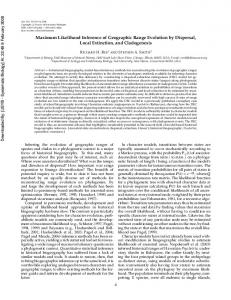
Data example

We illustrate RICF using data from Romney et al. [51] on the quality of life of n = 469 cardiac patients. The path diagram in Figure 2 encodes a model for four variables: symptoms of illness (Y1 ), diminished socioeconomic status (SES) (Y2 ), low morale (Y3 ), and poor interpersonal relationships (Y4 ). The parameters to estimate are β21 , β31 , β32 , β43 and ω11 , ω22 , ω33 , ω44 , ω24 . Vertex 1 in Figure 2 has no parents and spouses. Hence, its RICF update step consists of a trivial regression. In other words, the conditional variance ω11 is in fact the unconditional variance of Y1 with 16

1

3

2

4

Figure 2: Path diagram for variables measuring patient quality of life: symptoms of illness (1), diminished SES (2), low morale (3), and poor relationships (4). Y1

i=2

1

3 β21

2

4

ω24

Y2

i=3

Z4 Y3 3

β31 1 β32 2

4

Y2

i=4

Y3 3

1

2

ω24

Z2

β43 4 Y4

Figure 3: Illustration of the ICF update steps for i = 2, 3, 4. For each step, the structure of the least squares regression is indicated by directed edges pointing from the predictor variables to the response variable depicted by a square node. (See text for details.) MLE ω ˆ 11 = s11 . For the remaining vertices, the corresponding update steps of the RICF algorithm are illustrated in Figure 3. Here, the response variable Yi in the i-th update step is shown as a square node while the remaining variables are depicted as circles. Variables acting as covariates are labelled either by Yj or by Zj depending on whether the random variable Yj , or the pseudo-variable Zj defined in (4.4) is used in the regression. Finally, directed edges point from a covariate Yj or Zj to the response Yi to indicate the structure of the least squares regression that has to be performed in the i-th RICF step. Since vertex 3 has no spouses, the MLEs of β31 , β32 , and ω33 are given by the regression estimates βˆ31 = s31 /s33 , βˆ32 = s32 /s33 , and ω ˆ 33 = s33 − s232 /s33 , respectively. Thus the repetition of steps 1 to 5 in §4.1 are required only for i ∈ {2, 4}. Romney et al. [51] summarized their data in a correlation matrix. For illustration purposes, we applied the RICF algorithm to this correlation matrix but we note that the data analysis should instead be based on the empirical covariance matrix. Using the identity matrix as a starting value for Ω, we iterated RICF until convergence, which was reached after only four iterations. The resulting estimates are given in Table 2. Although there are no general guarantees ensuring that the estimates constitute the global maximum of the likelihood function, the small value of 0.08 for the deviance of N(G) indicates a good fit when compared to the two degrees of freedom.

17

Table 2: Maximum likelihood estimates and their standard errors computed from the Fisher-information. Parameter MLE SE β21 0.34 0.05 β31 0.48 0.05 β32 0.14 0.04 β43 0.53 0.05 ω11 1.00 0.07 ω22 0.88 0.06 ω33 0.70 0.06 ω44 0.73 0.06 ω24 -0.07 0.04 1 4

5

3

2

Figure 4: Path diagram inducing seemingly unrelated regressions.

5

Conclusion

After giving examples of multivariate linear models induced by path diagrams that are not curved exponential families, we turned to linear models based on what we called bow-free acyclic path diagrams (BAPs). In Theorem 2.9, our first main result, we show that BAPs induce models that are everywhere identifiable. This result extends a previous identifiability result of Brito and Pearl [8] that held only almost everywhere. As Corollary 2.10, we obtain the important result that bow-free acyclic path diagrams always induce curved exponential families. We then turned to likelihood inference in bow-free acyclic models. After stating likelihood equations and Fisher-information, we devised the Residual Iterative Conditional Fitting (RICF) algorithm for solving the likelihood equations. The iterations of RICF consist of maximizing the log-likelihood function varying some parameters while holding other parameters fixed and are based on the decomposition of the log-likelihood function presented in Theorem 4.1. Besides clear convergence properties stated in Theorem 4.2, the RICF algorithm has the attractive feature that parameters will be estimated in a single cycle if this is possible. In particular, if applied to a model based on an acyclic directed graph (DAG), the algorithm converges in a single cycle and performs exactly the regressions commonly used for fitting multivariate normal DAG models. This feature and the fact that RICF can be implemented using nothing but least squares computations make it an attractive alternative to the less specialized optimization methods commonly used in modelling with path diagrams. In another special case, namely seemingly unrelated regressions, RICF reduces to the algorithm of Telser [62]. An example of a path diagram representing seemingly unrelated regressions is shown in Figure 4. The variables Y1 , Y2 and Y3 are then commonly thought of as covariates. Since they have no spouses, the MLEs of the variances ω11 , ω22 and ω33 are equal to the empirical variances s11 , s22 and s33 . The update steps of RICF for the remaining variables Yi , i = 4, 5, are regressions on both the “covariates” Ypa(i) and the residual εj , j ∈ {4, 5} \ {i}. These are exactly the updates used in Telser’s algorithm. It follows that our results on RICF clarify in particular the convergence guarantees for Telser’s algorithm. 18

As presented, RICF is dependent upon the exact structure of the path diagram G. However, different path diagrams may impose the same statistical model; a trivial example being the three graphs 1 → 2, 2 → 1, and 1 ↔ 2 that all induce a saturated model for two variables Y1 and Y2 . In larger examples, this equivalence may be exploited to find the ‘best path diagram’ to run RICF, but it is currently still an open problem how to find such a ‘best path diagram’ in general. Acknowledgements Mathias Drton was supported by NSF grant DMS 0505612. Thomas Richardson acknowledges support by NSF grant DMS 0505865.

References [1] Ali, R. A., Richardson, T. and Spirtes, P. (2004). Markov equivalence for ancestral graphs. Tech. Rep. 466, Dept. of Statistics, University of Washington. [2] Andersson, S. A., Madigan, D. and Perlman, M. D. (1997). A characterization of Markov equivalence classes for acyclic digraphs. Ann. Statist. 25 505–541. [3] Bekker, P., Meckens, A. and Wansbeek, T. (1994). Identification, Equivalent Models, and Computer Algebra. Academic, Boston. [4] Bentler, P. M. (1986). Theory and Implementation of EQS: A Structural Equations Program. BMDP Statistical Software, Los Angeles. [5] Blalock, H. (1962). Four variable causal models and partial correlations. American Journal of Sociology 68 182–194. [6] Bollen, K. A. (1989). Structural Equations with Latent Variables. Wiley, New York. [7] Box, G. (1966). Use and abuse of regression. Technometrics 8 625–629. [8] Brito, C. and Pearl, J. (2002). A new identification condition for recursive models with correlated errors. Struct. Equ. Model. 9 459–474. [9] Browne, M. (1984). Asymptotically distribution-free methods for the analysis of covariance structures. British J. Math. Statist. Psych. 37 62–83. [10] Chaudhuri, S., Drton, M. and Richardson, T. S. (2006). Estimation of a covariance matrix with zeros. Biometrika accepted. [11] Cox, D., Little, J. and O’Shea, D. (1997). Ideals, Varieties, and Algorithms, 2nd ed. Springer-Verlag, New York. [12] Cox, D. R. and Wermuth, N. (1996). Multivariate Dependencies: Models, Analysis and Interpretation. Chapman and Hall, London. [13] Dawid, A. (2000). Causal inference without counterfactuals (with discussion). J. Amer. Statist. Assoc. 95 407–448. [14] Drton, M. (2006). Computing all roots of the likelihood equations of seemingly unrelated regressions. J. Symbolic Comput. 41 245–254. [15] Drton, M. and Eichler, M. (2006). Maximum likelihood estimation in Gaussian chain graph models under the alternative Markov property. Scand. J. Statist. 33 247–257. [16] Drton, M. and Richardson, T. S. (2004). Graphical answers to questions about likelihood inference for Gaussian covariance models. Tech. Rep. 467, Dept. of Statistics, University of Washington. [17] Drton, M. and Richardson, T. S. (2004). Multimodality of the likelihood in the bivariate seemingly unrelated regressions model. Biometrika 91 383–392. [18] Epstein, R. (1987). A History of Econometrics. North Holland, Amsterdam. [19] Fisher, F. (1966). The Identification Problem in Econometrics. McGraw-Hill, New York. [20] Fisher, F. (1970). A correspondence principle for simultaneous equation models. Econometrica 38 73–92. [21] Fletcher, R. and Powell, M. (1963). A rapidly convergent descent algorithm for minimization. Computer J. 6 163–168.

19

[22] Geiger, D., Heckerman, D., King, H. and Meek, C. (2001). Stratified exponential families: graphical models and model selection. Ann. Statist. 29 505–529. ¨ nemann, H. (2005). Singular 3.0. A Computer Alge[23] Greuel, G.-M., Pfister, G. and Scho bra System for Polynomial Computations, Centre for Computer Algebra, University of Kaiserslautern. http://www.singular.uni-kl.de. [24] Haavelmo, T. (1943). The statistical implications of a system of simultaneous equations. Econometrica 11 1–12. [25] Harville, D. A. (1997). Matrix Algebra from a Statistician’s Perspective. Springer-Verlag, New York. [26] Haughton, D. M. A. (1988). On the choice of a model to fit the data from an exponential family. Ann. Statist. 16 342–355. ¨ reskog, K. G. and So ¨ rbom, D. (1995). LISREL 8: User’s Reference Guide. Scientific Software [27] Jo International, Chicago. [28] Kass, R. E. and Vos, P. W. (1997). Geometrical Foundations of Asymptotic Inference. Wiley, New York. [29] Kiiveri, H. T. (1987). An incomplete data approach to the analysis of covariance structures. Psychometrika 52 539–554. [30] Koster, J. T. A. (1999). Linear structural equations and graphical models. Lecture notes, The Fields Institute, Toronto. [31] Koster, J. T. A. (1999). On the validity of the Markov interpretation of path diagrams of Gaussian structural equation systems with correlated errors. Scand. J. Statist. 26 413–431. [32] Lauritzen, S. L. (1996). Graphical Models. Clarendon Press, Oxford, UK. [33] Lauritzen, S. L. (2001). Causal inference from graphical models. In Complex Stochastic Systems (O. E. Barndorff-Nielsen, D. R. Cox and C. Kl¨ uppelberg, eds.). Chapman & Hall, Boca Raton, FL, 63–107. [34] Lauritzen, S. L. and Richardson, T. S. (2002). Chain graph models and their causal interpretations (with discussion). J. R. Stat. Soc. Ser. B 64 321–361. [35] Lee, S. and Hershberger, S. (1990). A simple rule for generating equivalent models in covariance structure modelling. Multivariate Behavioral Research 25 313–334. [36] MacCallum, R., Wegener, D., Uchino, B. and Fabrigar, L. (1993). The problem of equivalent models in applications of covariance structure analysis. Psychological Bulletin 114 185–199. [37] McDonald, R. (2002). What can we learn from the path equations?: Identifiability, Constraints, Equivalence. Psychometrika 67 225–249. [38] Morgan, M. S. (1991). The stamping out of process analysis in econometrics. In Appraising Economic Theories (N. de Marchi and M. Blaug, eds.). Edward Elgar, Cheltenham, 237–272. [39] Nelson, C. and Startz, R. (1990). The distribution of the instrumental variables estimator and its t-ratio when the instrument is a poor one. Journal of Business 63 S125–40. [40] Nelson, C. and Startz, R. (1990). Some further results on the exact small sample properties of the instrumental variables estimator. Econometrica 58 967–76. [41] Neyman, J. (1923). Sur les applications de la théorie des probabilités aux experiences agricoles: Essai des principes. Roczniki Nauk Rolniczych X 1–51. In Polish, English translation by D. Dabrowska and T. Speed in Statistical Science 5 463–472, 1990. [42] Niles, H. (1922). Correlation, causation and Wright theory of path coefficients. Genetics 7 258–273. [43] Pachter, L. and Sturmfels, B. (2005). Algebraic Statistics for Computational Biology. Cambridge University Press, Cambridge, UK. [44] Pearl, J. (1988). Probabilistic Reasoning in Intelligent Systems. Morgan Kaufmann, San Mateo, CA. [45] Pearl, J. (1995). Causal diagrams for empirical research (with discussion). Biometrika 82 669–690. [46] Pearl, J. (2000). Causality: Models, Reasoning, and Inference. Cambridge University Press, Cambridge, UK. [47] Raftery, A. E. (1993). Bayesian model selection in structural equation models. In Testing Structural Equation Models (K. Bollen and J. Long, eds.). Sage Publications, Newbury Park, 163–180. [48] Raykov, T. and Penev, S. (1999). On structural equation model equivalence. Multivariate Behavioral Research 34 199–244.

20

[49] Richardson, T. S. and Spirtes, P. (2002). Ancestral graph Markov models. Ann. Statist. 30 962–1030. [50] Rindskopf, D. (1984). Structural equation models: Empirical identification, Heywood cases, and related problems. Sociol. Methods Res. 13 109–119. [51] Romney, D., Jenkins, C. and Bynner, J. (1992). A structural analysis of health-related quality of life dimensions. Human Relations 45 165–176. [52] Rubin, D. (1974). Estimating causal effects of treatments in randomized and non-randomized studies. Journal of Educational Psychology 66 688–701. [53] Shafer, G., Kogan, A. and Spirtes, P. (1993). Generalization of the tetrad representation theorem. Tech. Rep. 26-93, Rutgers Center for Operations Research, Rutgers University. [54] Shapiro, A. (1986). Asymptotic theory of overparameterized structural equation models. J. Amer. Statist. Assoc. 81 142–149. [55] Spearman, C. (1904). General intelligence, objectively determined and measured. American Journal of Psychology 15 201–293. [56] Spirtes, P., Glymour, C. and Scheines, R. (2000). Causation, Prediction, and Search, 2nd ed. MIT Press, Cambridge, MA. [57] Spirtes, P., Richardson, T., Meek, C., Scheines, R. and Glymour, C. (1998). Using path diagrams as a structural equation modelling tool. Sociol. Methods Res. 27 182–225. [58] Steiger, J. H. (2001). Driving fast in reverse. J. Amer. Statist. Assoc. 96 331–338. [59] Stelzl, I. (1986). Changing a causal hypothesis without changing the fit: some rules for generating equivalent path models. Multivariate Behavioral Research 21 309–331. [60] Stock, J., Wright, J. and Yogo, M. (2002). A survey of weak instruments and weak identification in generalized method of moments. J. Bus. Econom. Statist. 20 518–29. [61] Strotz, R. and Wold, H. (1960). Recursive versus non-recursive systems: An attempt at synthesis. Econometrica 28 417–427. [62] Telser, L. G. (1964). Iterative estimation of a set of linear regression equations. J. Amer. Statist. Assoc. 59 845–862. [63] Turner and Stevens (1959). The regression analysis of causal paths. Biometrics 15 236–258. [64] Wang, J. and Zivot, E. (1998). Inference on structural parameters in instrumental variables regression with weak instruments. Econometrica 66 1389–404. [65] Wermuth, N. (1980). Linear recursive equations, covariance selection, and path analysis. J. Amer. Statist. Assoc. 75 963–972. [66] Wermuth, N. (1992). On block-recursive regression equations (with discussion). Braz. J. Probab. Stat. (Revista Brasileira de Probabilidade e Estatistica) 6 1–56. [67] Whittaker, J. (1990). Graphical Models in Applied Multivariate Statistics. Wiley, Chichester. [68] Wold, H. and Bentzel, R. (1946). On statistical demand analysis from the viewpoint of simultaneous equations. Skandinavisk Aktuarietidskrift 29 95–114. [69] Wold, H. and Jur´ een, L. (1953). Demand Analysis. Wiley, New York. [70] Wothke, W. (1993). Nonpositive definite matrices in structural modelling. In Testing Structural Equation Models (K. Bollen and J. Long, eds.). Sage Publications, Newbury Park, 256–293. [71] Wright, S. (1921). Correlation and causation. Journal of Agricultural Research 20 557–585. [72] Wright, S. (1923). The theory of path coefficient. A reply to Niles’s criticism. Genetics 8 239–55. [73] Wright, S. (1934). The method of path coefficients. Ann. Math. Statist. 5 161–215. [74] Zhang, J. and Spirtes, P. (2005). A characterization of Markov equivalence classes for ancestral graphical models. Tech. Rep. 168, Dept. of Philosophy, Carnegie-Mellon University.

A

Singularities

Example 2.2 (cont.). We take up the example of the cyclic path diagram G depicted in Figure 1(a). As stated in Example 2.2 in Section 2 the parameter space P(G) of the model N(G) constitutes part of 21

a hypersurface defined by an irreducible polynomial f of degree 6. Using techniques from computational algebraic geometry implemented in Singular [23], we can compute the singular locus [11, p. 479] of this hypersurface. The intersection of this singular locus with the parameter space P(G) is equal to the set of matrices {Σ ∈ P(G) | σ13 = σ14 = 0}. From this set we can choose covariance matrices Σ at which the parameters B and Ω are not identifiable, and at which the set P(G) is not diffeomorphic to Rdim(P(G)) = R9 . Hence, the set P(G) is not a smooth manifold in the cone of positive definite matrices and the model N(G) is not a curved exponential family. Consider, for example, the covariance matrix   1 1 0 0  1 7 4 7  Σ0 =   0 4 3 5 . 0 7 5 9

The matrix Σ0 is in P(G) because it can  0 0 1 0 B= −1 1 0 0

be expressed as Σ0 = Φ(B, Ω) using the matrices    1 0 0 0 0 0 0 1 0 0 0 1  ,  Ω = 0 0 1 0 . 0 0 0 0 0 1 2 0

¯ Ω) ¯ with However, the matrix Σ0 is also equal to Σ0 = Φ(B,     1 0 0 0 0 0 0 0   0  0 0 2/3  , ¯ = 0 2/3 0 ¯= 1 Ω B 0 0 1/2 0  . −1/2 1/2 0 0  0 0 0 3/4 0 0 3/2 0

Hence, the model N(G) is not everywhere identifiable. Using the two representations Σ0 = Φ(B, Ω) = ¯ Ω) ¯ we can also contradict the hypothesis that the model N(G) is a curved exponential family. Φ(B, If the hypothesis was true, then the set P(G) may have at most dim(P(G)) = 9 linearly independent tangent vectors at the point Σ0 . However, we can find 10 linearly independent tangent vectors as follows. ¯ Ω). ¯ Then Compute the 9 × 10 Jacobi matrix of the mapping Φ and evaluate it both at (B, Ω) and (B, append the two matrices to form a 18 × 10 matrix J. Each row of J gives a tangent vector for P(G) at Σ0 . Now, the rank of J is equal to 10, which says that there are 10 linearly independent tangent vectors at Σ0 . Example 2.7 (cont.). We take up the example of the cyclic path diagram G depicted in Figure 1(b). As stated in Example 2.7 in Section 2 the parameter space P(G) of the model N(G) is embedded in a hypersurface defined by a quadratic polynomial f known as tetrad. The intersection of the singular locus of this hypersurface with the parameter space P(G) is equal to {Σ ∈ P(G) | σ13 = σ14 = σ23 = σ24 = 0}. We note that the singularities in this model are closely related to the problems associated with ‘weak instruments’ in econometrics [39, 40, 60, 64]. As in the above cyclic example, we can choose covariance matrices Σ at which the parameters B and Ω are not identifiable, and which lead to contradiction with the hypothesis that the model N(G) is a curved exponential family. For example, consider the covariance matrix   1 1 0 0  1 2 0 0  Σ0 =   0 0 2 1 . 0 0 1 3 22

It holds that Σ0 = Φ(B, Ω) with  0 1 B= 0 0 ¯ Ω) ¯ with Alternatively, Σ0 = Φ(B,  0 1 ¯= B 0 0

0 0 0 0

0 0 0 1

0 0 0 0 0 0 0 1/2

 0 0 , 0 0



1 0 Ω= 0 0  1 0 ¯ = Ω 0 0

 0 0 , 0 0

 0 0 0 1 0 0 . 0 2 −1 0 −1 3 0 1 0 0

 0 0 0 0  . 2 0  0 5/2

This shows that the model N(G) is not everywhere identifiable. Looking at the Jacobi matrix of the parameterization map Φ, as in Example 2.7 above, allows us to obtain 10 linearly independent tangent vector of P(G) at Σ0 . This yields that the model N(G) cannot be a curved exponential family as dim(P(G)) = 9 < 10.

23