This article has been accepted for inclusion in a future issue of this journal. Content is final as presented, with the exception of pagination. IEEE TRANSACTIONS ON AUTOMATION SCIENCE AND ENGINEERING
1
Image-Based Process Monitoring Using Low-Rank Tensor Decomposition Hao Yan, Kamran Paynabar, Member, IEEE, and Jianjun Shi
Abstract—Image and video sensors are increasingly being deployed in complex systems due to the rich process information that these sensors can capture. As a result, image data play an important role in process monitoring and control in different application domains such as manufacturing processes, food industries, medical decision-making, and structural health monitoring. Existing process monitoring techniques fail to fully utilize the information of color images due to their complex data characteristics including the high-dimensionality and correlation structure (i.e., temporal, spatial and spectral correlation). This paper proposes a new image-based process monitoring approach that is capable of handling both grayscale and color images. The proposed approach models the high-dimensional structure of the image data with tensors and employs low-rank tensor decomposition techniques to extract important monitoring features monitored using multivariate control charts. In addition, this paper shows the analytical relationships between different low-rank tensor decomposition methods. The performance of the proposed method in quick detection of process changes is evaluated and compared with existing methods through extensive simulations and a case study in a steel tube manufacturing process. Note to Practitioners—This paper, motivated by the problem of combustion monitoring in steel tube manufacturing, focuses on the development of effective methods for process monitoring based on image data. Existing process monitoring techniques cannot fully utilize the information of color images due to the high-dimensionality and complex correlation structure of such data. This paper addresses this problem by extracting essential monitoring features, while considering the spatial and spectral correlation of color images. This is accomplished by using various low-rank tensor decomposition methods along with multivariate control charts. The proposed approach can lead to a computer-aided online monitoring system for automatic detection of out-of-control situations in a process. Using simulation, the performance of the developed methods is compared under various scenarios. This can provide practitioners with useful guidelines for selecting an appropriate method for image-based process monitoring. In future research, we will study the development of image-based fault diagnosis techniques that can be integrated with the process monitoring approaches proposed in this paper. Index Terms—Average run length, control charts, image-based quality control, online monitoring, tucker and CP decompositions. Manuscript received June 21, 2013; revised January 21, 2014; accepted March 19, 2014. This paper was recommended for publication by Associate Editor W. Sheng and Editor J. Wen upon evaluation of the reviewers’ comments. (Corresponding author: Kamran Paynabar.) The authors are with the H. Milton Stewart School of Industrial and Systems Engineering, Georgia Institute of Technology, Atlanta, GA 30332-0205 USA (e-mail:
[email protected];
[email protected];
[email protected]). Color versions of one or more of the figures in this paper are available online at http://ieeexplore.ieee.org. Digital Object Identifier 10.1109/TASE.2014.2327029
I. INTRODUCTION
R
ECENT advancements in online sensing technologies have facilitated process monitoring in both manufacturing and service systems. Among various sensing techniques, image sensors have attracted special attention in process monitoring due to the rich process information provided by these sensors. Image-based process monitoring is being widely used in various applications including manufacturing processes [1], [2], food industries [3], medical decision-making [4], [5], and structural health monitoring [6]. For example, in steel tube manufacturing processes, the quality of combustion depends on the stability of both shape and color of the furnace flame that is controlled by adjusting the amount of the air and gas. Inadequate amounts of these substances results in an irregular shape and color of the flame, which may in turn affect the quality of the produced steel. To maintain the quality of combustion, the condition of the flame is monitored by a video camera. A sample of the flame image in this process is shown in Fig. 1(a). As another example in snack production processes, color images of snacks, shown in Fig. 1(b), are used to monitor the quality of coating concentration [3]. Traditionally, image data were analyzed through human-vision inspection. However, human-vision inspection is often slow and imprecise, which makes it an inefficient approach for monitoring processes with a high production or sampling rate. Consequently, the human-vision inspection was replaced by machine-vision systems, in which image acquisition, image analysis and decision-making are performed by computer systems [7]. In general, machine-vision systems share a common procedure that includes image acquisition, image preprocessing, feature extraction, and monitoring and control [8] (see Fig. 2). In this procedure, first, images are acquired using image sensors and cameras. Then, to prepare images for further analysis, a set of preprocessing methods including noise reduction, image registration, image compression, background separation, contrast enhancement, etc., were performed. Next, a set of monitoring features were extracted from each image, and finally, the extracted features are used to develop a statistical or engineering method for process monitoring and control. Most of the image-based process monitoring methods follow a similar procedure. Megahed et al. [9] provided a thorough review on imaged-based process monitoring methods. They categorized these methods into a few groups including multivariate and profile-based techniques, spatial control charts, and multivariate-image-analysis (MIA) control charts. In the first group, multivariate control charts along with a feature extraction
1545-5955 © 2014 IEEE. Personal use is permitted, but republication/redistribution requires IEEE permission. See http://www.ieee.org/publications_standards/publications/rights/index.html for more information.
This article has been accepted for inclusion in a future issue of this journal. Content is final as presented, with the exception of pagination. 2
Fig. 1. Samples of image data in manufacturing process. (a) Flame image in a steel manufacturing process. (b) Coating images in a snack production process (adopted from [3]).
Fig. 2. Combustion flame in a steel manufacturing process.
method such as principal component analysis (PCA) and profile modeling were used for process monitoring. For example, control chart Lin et al. [10] used the wavelet-Hoteling and wavelet-PCA approach to detect surface defects in light emitting diode chips using grayscale images. Wang and Tsung [11] modeled the relationship between a sampled image and a baseline by using Q-Q plots and then, used profile-monitoring methods to detect changes in these plots. A major disadvantage of this method is that it ignores the information about pixel locations. The spatial control charts, however, consider the spatial information by using non-overlapping windows that move across an image [12]. Lu and Tsai [13] used the singular value decomposition (SVD) to decompose an image of a liquid crystal display (LCD) panel into a low-rank background texture
IEEE TRANSACTIONS ON AUTOMATION SCIENCE AND ENGINEERING
and sparse spatial defects on the LCD panel. Jiang et al. [14] developed an ANOVA-based technique for monitoring the uniformity of LCD panels and used an exponentially weighted moving average (EWMA) control chart to detect the size and location of defects. The main disadvantage of profile-based and spatial monitoring methods is that these methods are typically applicable to grayscale images and they cannot be directly used for the monitoring of color images. MIA techniques, on the other hand, can handle color images by extracting features from each color channel. Yu and MacGregor [3] used MIA to monitor the coating density of snacks and flame images. Wood et al. [15] and Sbárbaro and Villar [16] utilized MIA to analyze spectroscopic images. Although, MIA can effectively extract color features, it neglects the spatial information of an image [8]. An extension of MIA, called multi-resolution multivariate image analysis (MR-MIA), can extract both color and texture features [17]. However, MR-MIA is not effective when a strong interaction exists between the color and texture. Low-rank decomposition methods like PCA have been traditionally used for feature extraction and analysis of high-dimensional data such as nonlinear profiles and images, (see, for example, the work by Yeung and Ruzzo [18] and Ye et al. [19]). However, the application of the regular PCA is limited to vectors and matrices, and cannot be applied to color images that are characterized by multidimensional arrays. One approach to overcome this limitation is to unfold the image data to a vector and then, apply regular PCA to unfolded images. For example, a sample of Red, Green, and Blue (RGB)-color images with 3 could turn into a vector of size 1. dimensions of Henceforth, this method is referred to as “unfolded-PCA (UPCA).” Although UPCA has been used in various image processing applications (see, for example, Liu and MacGregor [17], Bharati et al. [20]), there are several issues in applying UPCA to color image data. Besides the high computational complexity of UPCA induced by unfolding images, this approach breaks the correlation structure of image data and thus, loses potentially more compact representations that can be obtained in the original form [19]. Low-rank tensor decomposition (LRTD) is an alternative to the UPCA that addresses these deficiencies. A tensor is defined as a multidimensional array. For example, an RGB-color image with dimensions of 3 can be viewed as an order-3 tensor. Unlike UPCA, LRTD methods, such as tensor-based PCA directly analyze a tensor without unfolding it into a vector, thus preserving the tensor structure of the original object. The tensor-based PCA was applied to various applications such as face recognition [21], gait classification [22], electroencephalography, functional magnetic resonance imaging analysis [23], and process monitoring. Louwerse and Smilde [24] and Hu and Yuan [25] used tensor-based PCA to monitor batch-to-batch variations. Paynabar et al. [26] used tensor-based PCA along with hierarchical classification to detect and diagnose different fault types in forging processes. Although LRTD techniques have been used in various areas, their applications to image-based process monitoring is yet to be studied. Moreover, LRTD methods have been studied in various fields such as Mathematics and Computer Science. The literature in these areas, in some way, is disconnected and the relationship among LRTD methods developed in each field still remains unclear.
This article has been accepted for inclusion in a future issue of this journal. Content is final as presented, with the exception of pagination. YAN et al.: IMAGE-BASED PROCESS MONITORING USING LOW-RANK TENSOR DECOMPOSITION
The main objective and contribution of this paper is to develop image-based monitoring methods that effectively utilize the spatial and color information of image data by using LRTD methods. Using extensive simulations, the performance of the proposed image-based monitoring methods are evaluated under various scenarios. This can provide practitioners with useful guidelines for selecting an appropriate method for image-based process monitoring. Furthermore, the connection between various LRTD methods is studied in this paper. The remainder of this paper is organized as follows. Section II provides an overview of the basic notations and definitions in multilinear algebra. Section III gives a brief overview of different image feature extraction and dimension reduction methods including UPCA, MIA, multilinear PCA (MPCA), uncorrelated multilinear PCA (UMPCA), and tensor rank-one decomposition (TROD). Section IV studies the relationships of the foregoing methods. In Section V, an image-based monand control charts is proposed itoring method based on which utilizes extracted features from different low-rank decomposition methods. In Section VI, an extensive simulation study was performed to evaluate and compare the performance of different feature extraction and monitoring methods based on symmetric and asymmetric images. A real case study of flame monitoring in a steel tube manufacturing process was conducted in Section VII. Finally, Section VIII was devoted to conclusions and future research. II. BASIC NOTATIONS AND DEFINITIONS MULTILINEAR ALGEBRA
IN
In this section, we introduce basic notations, definitions, and operators in multilinear algebra that we used for tensor analysis. Throughout this paper, scalars are denoted by lowercase italic letters, e.g., , vectors by lowercase boldface letters, e.g., , matrices by uppercase boldface letter, e.g., , and -order tensor is tensors by calligraphic letters, e.g., . An represented by and is addressed by indices . represents the dimension of the -mode of , in which a -mode vector is defined as a vector obtained by varying , while keeping other by a matrix indices fixed. The -mode product of a tensor is defined by A rank-one tensor can be represented by outer products of vectors, i.e., , where is an – dimension vector and is the outer product operator. The scalar is defined product of two tensors and as is computed by . the Frobenius norm of Suppose is an matrix and is a matrix. Then, the Kronecker product of these matrices, de, is the block matrix defined by noted by .. .
..
.
.. .
. The Khatri–Rao product
is the matching-column-wise Kronecker product. Given and , their Khatri–Rao matrices is a matrix and defined product denoted by . The by
3
Fig. 3. Illustration of 1-mode vectors and 1-mode unfolding.
-mode unfold of a tensor
is a matrix represented by . The columns of are the -mode vectors of . A visual illustration of 1-mode unfolding and 1-mode vectors of a third-order tensor was shown in Fig. 3. The higher order singular value decomposition (HOSVD) of , also known as Tucker decoma tensor , position, is defined as is an orthogonal where matrix and is the core tensor [27], [28]. Also, the CANDECOMP/PARAFAC (CP) decomposition of the tensor is defined as , is an -dimension vector and is a singular where value [29]. Similar to the SVD, the CP factorizes a tensor into a sum of rank-one arrays, but they are not orthogonal. Finally, we define the vec(•) operator to reshape a tensor to a vector. For , is obtained by una tensor -mode. That is , folding along the -dimension vector. which is an III. METHODS OF DIMENSION REDUCTION FOR IMAGE DATA In this section, we review various low-rank decomposition techniques that can be used for image dimension reduction and features extraction. Specifically, UPCA, MPCA, UMPCA, and TROD methods are introduced. A. Unfold Principal Component Analysis (UPCA) As mentioned earlier, PCA can only be applied to the matrixstructured data. The UPCA, however, is a generalization of PCA that can be used for dimension reduction in tensor data. Let denote a sample of images, where and are the number of horizontal and vertical image pixels, respectively, and is the number of color channels. For example, is 1 for grayscale and it is 3 for RGB-color images. In the UPCA, the is turned into an sample of images matrix by unfolding the tensor along the 4-mode. Then, the PCA algorithm is applied to the unfolded tensor denoted . Solving the following eigen-decomposition problem by gives the loadings matrix of PCA:
where is the centered , i.e., , is the orthonormal matrix of eigenvectors and is a diagonal . matrix consisting of the eigenvalues of Consequently, the matrix of PC-scores (PC-features) denoted into the subspace , by can be obtained by projecting is an matrix comprising columns of where matrix , that is . Also, the residual matrix is calculated by .
This article has been accepted for inclusion in a future issue of this journal. Content is final as presented, with the exception of pagination. 4
IEEE TRANSACTIONS ON AUTOMATION SCIENCE AND ENGINEERING
MIA is another form of UPCA that has been widely used for analyzing color images. The main purpose of the MIA is to find a low-rank representation of images in color subspace. Thus, the is unfolded along the 3-mode, image sample which is the color channels. Then, the PCA algorithm is applied to the non-centered estimate of the covariance matrix, calcu. The major deficiency of lated by MIA is that it cannot utilize the spatial information of pixels and thus cannot effectively detect changes in the area and shape of objects.
The alternative least square algorithm (ALS) [29], [31] can be used to solve the optimization model in (2). More details on CP decomposition can be found in [29]. ; For a sample of in-control images, i.e., , one can use the TROD as follows:
B. Multilinear Principal Component Analysis (MPCA)
(3)
An alternative approach to UPCA is to use multilinear algebra methods by performing dimension reduction directly on tensors rather than unfolded data. MPCA, introduced by Lu et al. [30], is one of the multilinear dimension reduction techniques applicable to tensor data. The MPCA algorithm for image data in-conis summarized as follows. For a training sample of ; , the trol images, denoted by MPCA objective is to find a set of orthogonal transformation matrices such that the projected low-dimensional tensor captures the most of variation observed in the original tensor. Let denote the low-dimensional tensor after projection. The MPCA model is formalized as follows: (1) where and is the centered , i.e., . If is used instead of in (1), the method is defined as non-centered MPCA. In this paper, we apply the non-centered MPCA as our feature extraction method. Lu et al. [30] proposed an iterative algorithm for solving the optimization model in (1). It should be noted that the extracted features by MPCA are correlated. More details on the MPCA model can be found in Lu et al. [30]. C. Tensor Rank-One Decomposition (TROD) and Candecomp/Parafac (CP) Decomposition The CP decomposition is another multilinear algebra method that can be used for image dimension reduction and feature extraction. The CP decomposition factorizes a tensor as a sum of a few rank-one tensors [29], [31]. The CP decomposition of a using rank-one tensors is repcolor image resented as with ; , where is an -dimension is a singular value. Although like SVD, the vector and CP decomposes the data into sum of rank-one arrays, these rank s are obtained by one arrays are not orthogonal. Given , solving the following optimization model:
(2)
More details on TROD can be found in [32]. D. Uncorrelated Multilinear Principal Component Analysis (UMPCA) The UMPCA was introduced by Lu et al. [33] to overcome the problem of correlated features in MPCA. UMPCA follows the classical PCA derivation of successive variance maximization to enforce the uncorrelated feature [34]. In UMPCA, a number of elementary multilinear projections are solved one by one to maximize the captured variance. To formulate the ; be a UMPCA problem, let , training sample, and be the PC-score, which is the projection of the sample into the subspace . as the coordinate of projection into the Denote coordinate of the sample. The projection vectors, also known as elementary multilinear projections (EMP) can be computed by
subject to ; and ; , More details on UMPCA can be found in Lu et al. [33]. The UMPCA projects a tensor into orthogonal vectors. However, because of imposing the orthogonality constraint into , the number of PC-features is limited by . For example, in color images , means that the number of features is with limited to three features. IV. RELATIONSHIP BETWEEN METHODS In Section III, we reviewed several existing dimension reduction methods in the literature that can be used for image data. In this section, we study the connection between Tucker and MPCA, and between the TROD and CP through the following two propositions. Proposition 1: Let denote a centered tensor of a sample of images. The transformation matrices obtained by the following Tucker decomposition of are the same as the solutions to the MPCA model in (1):
(4)
This article has been accepted for inclusion in a future issue of this journal. Content is final as presented, with the exception of pagination. YAN et al.: IMAGE-BASED PROCESS MONITORING USING LOW-RANK TENSOR DECOMPOSITION
where . Proof is given in Appendix A. Proposition 2: Let denote a tensor comprising a sample of images, i.e., . Also, suppose that the CP decomposition of obtained from (2) . Then, is represented by the solutions to the CP decomposition model in (3) are given by ; and , where is the element of . Proof is given in Appendix B. The above propositions indicate that the CP and TROD are essentially the same, and one can use the MPCA to solve the Tucker decomposition. Therefore, we exclude the CP and Tucker in subsequent sections. V. MONITORING METHODS In this section, we propose a monitoring procedure by integrating the LRTD with control charts. First, we discuss how to define monitoring features for each LRTD method.
5
. The feature vector
is
given by
(5)
To solve the optimization model in (5), we rewrite it in a vector form by using Khatri–Rao product notation. (6) where . The optimization model in (6) has a closed-form solution that can be obtained by , where . Also, the residual tensor for the new image is calculated by . For TROD, the set of monitoring features is defined as and . D. Monitoring Features for UMPCA
A. Monitoring Features for UPCA Model For a new image , the UPCA features and residuals are calculated by and , respectively. Although the UPCA has been extensively used in the analysis of image data, it is not an effective dimension reduction technique for tensor data as it breaks the structure of tensor and has high computational complexity [35]. B. Monitoring Features for MPCA Method , the feature is calculated For a new image and residuals are obby . tained by operator For the purpose of process monitoring, we use to vectorize both and , and define and as monitoring features. C. Monitoring Features for TROD Method As can be seen from (3), all images share the same rank one arrays , but each image has its own singular value, i.e., , which represents differences values can among images. Thus, as would be shown later, be used as monitoring features. In order to solve the CP decomposition for multiple samples in (3), the following proposition is used. In addition, the monitoring features for a new image can be calculated by the following procedure. Suppose are solutions to the CP optimization model in (3), obtained from a training sample . The rank-one arrays estimated from the training sample, i.e., are used to calculate the features vector for , denoted by a new image
Suppose we have a new image UMPCA features are calculated by
, the
where is the estimated projection vectors from a training sample. It should be noted that residuals cannot be defined for UMPCA as it is a tensor to vector projection method. After defining all the features for control chart, any multivariate control charts including Hoteling control chart, Multivariate Cumulative Sum (MCUSUM), Multivariate Exponentially Weighted Moving Average (MEWMA), etc., can be used to monitor the extracted features. In this paper, we use Hoteling control chart [36]. Although low-rank features contain most of the image information, there also exists some process information in residuals that is not captured by the low-dimensional features. Consequently, we also monitor the residuals using -charts introduced by Nomikos and MacGregor [37]. In this paper, we focus on the phase II of process monitoring. Thus, it is assumed that a sample of images collected from an in-control process is available. First, the in-control samples are used to estimate LRTD models, and compute the control limits of and charts. Then, for each new image, the estimated decomposition models are used to extract features and residuals, and plot the monitoring statistics on the constructed and control charts. Let denote the -dimension vector of extracted features from a new image. The monitoring statistic can be defined as , where and , respectively, are the mean and the covariance matrix of the features estimated by in-control samples [36]. Also, let denote the vector of residuals of a new image. The -chart monitoring statistics is calculated by . If features and residuals follow multivariate normal distributions, then and , respectively, follow an distribution with and degrees
This article has been accepted for inclusion in a future issue of this journal. Content is final as presented, with the exception of pagination. 6
IEEE TRANSACTIONS ON AUTOMATION SCIENCE AND ENGINEERING
of freedom, and a Chi-square distribution with degrees of freedom. The parameters and can be estimated using the method of moments. Specifically, and can be calculated by solving the following set of equations; and [37]. Consequently, the control limits for and -charts can be determined by the percentiles of the corresponding distributions. However, in some applications, the normality assumption of feature and residual distributions is not valid. In such cases, the empirical distributions of and statistics are estimated using the training in-control sample and the percentiles obtained from the empirical distributions are defined as control limits. The number of monitoring features can be determined based on the percentage of total variation explained by the extracted features. In this paper, we select the first features with the largest variances such that the cumulative proportion of variance explained by these features exceeds a specified threshold. For the UPCA, this is calculated by , where is the element of matrix . For the TROD and MPCA, the cumulative proportion of explained variation is given by , where with for MPCA and
for TROD [38].
VI. PERFORMANCE EVALUATION USING SIMULATION STUDY In this section, we conduct simulations to evaluate and compare the performance of the discussed LRTD techniques in process monitoring. We consider images with symmetric and asymmetric foregrounds and study four different out-of-control scenarios in which the location, area, shape, and color of the image foreground changed. The simulation study was conducted in two stages. In the first stage, 10,000 in-control samples were randomly generated and used to estimate the LRTD model and construct the corresponding baseline control charts. In the second stage, out-of-control samples were randomly generated. For each sample, the monitoring features and residuals were calculated by using the estimated model in the first stage, and were plotted on the corresponding control charts. This process was repeated until an out-of-control sample was detected by either of the control charts. We used the average run length (ARL), calculated from 1000 replications as the performance index. The control limits were determined so that the combined in-control ARLs of and charts for all methods are approximately 200. It should be noted that for UMPCA, only a chart was used as residuals cannot be defined for this method. Additionally, to assess the computational complexity of proposed methods for real-time monitoring, the average time spent for online monitoring including feature extraction for a new image, and the calculation and comparison of monitoring statistics with control limits was reported. The details and results of simulation study for both symmetric and asymmetric cases are discussed in the following sections. A. Case 1. Images With Symmetric Foreground The in-control samples generated in this simulation study were RGB-color images that consist of a red circle on a black background. Three sets of
parameters were used to randomly generate the circles. These parameters include a two-dimentional center location randomly generated from a normal distribution, i.e., , color parameters (RGB numbers) independently generated from normal distributions with mean and variances , and constant circle radius in horizontal and vertical directions, i.e., . In this simulation, the following four out-of-control scenarios with different change magnitudes were examined. 1) Scenario 1 (Location Change): The mean of the circle center was shifted according to 2) Scenario 2 (Area Change): In this scenario, both vertical and horizontal radius change proportionally to in-control radius, i.e., . Consequently, the relationship between out-of-control and in-control areas, respectively, denoted by and , is given by . 3) Scenario 3 (Shape Change): Change in the shape of the circle was created by increasing the axis radius and decreasing the axis radius according to and . Define the shape index as . Consequently, the relationship between in-control and out-of-control shape indices, respectively, denoted by and , is given by . 4) Scenario 4 (Color Change): The color mean of the circle was changed according to . For illustration purposes, a sample of in-control and out-ofcontrol images was shown in Fig. 4. B. Case 2. Images With Asymmetric Foreground In the asymmetric case, each in-control RGB image is and consists of two overlapped circles (one red and one green) on a black background. Similar to the symmetric case, three sets of parameters are used for generating in-control samples; Center locations, which are for circle 1 (red circle) and for circle 2 (green circle), color parameters that were independently generated from normal distributions with means and variances for circle 1 and means , and variances for circle 2, and finally, constant radius for circles 1 and 2, which are and , respectively. In the asymmetric case, we also considered the same out-ofcontrol scenarios discussed in the symmetric case including location, area, shape, and color changes. In each scenario, the same change magnitudes were applied to both circles. A sample of in-control and out-of-control images generated from each scenario was shown in Fig. 5. In both symmetric and asymmetric cases, and under each change scenario, the out-of-control ARLs associated with different change magnitudes were estimated based on 1000 simulation replications. The standard error of the ARL estimates in the worst case is less than 6.32. Figs. 6 and 7 illustrate the
This article has been accepted for inclusion in a future issue of this journal. Content is final as presented, with the exception of pagination. YAN et al.: IMAGE-BASED PROCESS MONITORING USING LOW-RANK TENSOR DECOMPOSITION
7
Fig. 5. Samples of in-control and out-of-control images with asymmetric foreground. Fig. 4. Samples of in-control and out-of-control images with symmetric foreground.
estimated ARL values of different methods for symmetric and asymmetric cases, respectively. In addition to the LRTD-based feature extraction methods, we also considered another simple benchmark method. In this method, we define in which is the average of all the in-control samples, and is the norm operator. We then simply constructed a control chart on as a benchmark. According to Figs. 6 and 7, all methods are comparable in detecting location changes in both symmetric and asymmetric cases. In the area change, the MPCA outperforms other methods especially in the asymmetric case. It also exhibits the best performance in quick detection of shape and color changes when the image is asymmetric. In the symmetric case, however, the TROD outperforms the MPCA in detecting shape and color changes. Overall, the MPCA and TROD are more effective methods in terms of the quick detection of process changes. This is because these two methods incorporate the tensor structure of images into the dimension reduction model. The
UPCA, on the contrary, unfolds an image into a vector, and thus fails to incorporate the spatial information. The performance of UMPCA is limited due to the fact that it cannot extract more than three features, which is not sufficient to capture the variation of images. The simple benchmark method lacks efficient feature selection and treats all image pixels with equal weights. Consequently, it does not perform well in most cases. The MPCA performs significantly better in the asymmetric case. This is because the interaction between spatial and color information is more significant when the foreground is asymmetric and MPCA can capture more variations when such an interaction exists. On the other hand, in the symmetric case, the TROD has lower ARLs as it decomposes an image to the sum of rank-one tensors with no interactions among eigenvectors. This approximately holds for symmetric foregrounds. The out-of-control ARLs of the UMPCA exhibit an increasing pattern in some scenarios such as shape and area changes. To explain this counterintuitive pattern, we calculated the mean and standard deviation of value for the UMPCA. The results indicate that when a change occurs, the mean of values increases, while their standard deviation decreases. The
This article has been accepted for inclusion in a future issue of this journal. Content is final as presented, with the exception of pagination. 8
IEEE TRANSACTIONS ON AUTOMATION SCIENCE AND ENGINEERING
TABLE I AVERAGE TIME SPENT FOR ONLINE MONITORING OF AN IMAGE
It is worth noting that the construction of control charts including the estimation of parameters and projection matrices, and determining control limits is an offline procedure and it is done only once before online monitoring. VII. IMAGE-BASED PROCESS MONITORING STEEL TUBE MANUFACTURING
Fig. 6. Out-of-control ARLs of low-rank decomposition methods under different change scenarios for images with symmetric foregrounds.
Fig. 7. Out-of-control ARLs of low-rank decomposition methods under different change scenarios for images with asymmetric foregrounds.
magnitude of the mean change is not large enough to lead to an out-of-control signal. Thus, the detection probability decreases and consequently, the out-of-control ARL increases. This is also because of the limited number of UMPCA features that cannot capture sufficient image variations. The average time spent for online monitoring of 1000 images is also reported in Table I. This includes the time required for feature extraction, and the calculation and comparison of monitoring statistics with control limits. As can be seen from Table I, even for the slowest method (i.e., TROD) it only takes on average 0.03 s to monitor a new image. This indicates that the proposed method is fast enough for real-time monitoring of most manufacturing processes with high production rates.
IN
In this section, the methodology discussed in Section V is applied to a case study of image-based process monitoring in steel tube manufacturing. Steel tubes are traditionally produced through the hot charge rolling process. In this process, using reheating furnaces, steel billets are heated up to about 1250 C, which is suitable for plastic deformation of steel and hence for the rolling mill. After rolling, the two ends of the rolled billet are welded together to produce the tube. A furnace often consists of preheating, heating, and soaking zones. In each zone, a burner is needed to heat up the billet to a target temperature, which depends on the type of the steel. If the combustion of the burner is not controlled well, the change of temperature may affect the final product quality. For example, the overheating of the steel billet will lead to excessive billet grain size or even local melt of the steel billet that will eventually grow into defects in the steel tube. A lower temperature will result in less plastic deformation of the steel billet, and thus, the change in the shape of final products. Therefore, it is imperative to monitor the combustion in steel tube manufacturing processes. In order to evaluate and compare the effectiveness of the proposed methods in the monitoring of the combustion process, we set up an experiment as follows. First, we let the combustion process run under the normal condition for 10 s in which and the amount of air and natural gas were set as 200 , respectively. Then, we reduced the amount of air 13.4 and let the process run under this condition for to 150 8 more seconds. During the experiment, a camera was setup to record the flame images at the rate of 20 images per second that resulted in 200 images from the in-control process and 160 images from the out-of-control process. Each image is an RGB-color image with the size of 300 700 pixels. Before implementing the image-based control charts, we performed some preprocessing on images. First, the background of images was removed [1] as it was irrelevant to the performance of the process. An example of in-control and out-of-control images after background removal was shown in Fig. 8(a) and (b), respectively. Next, we used the non-overlapping moving average technique with the window size of 5 to reduce image noise as well as between-image correlation. Consequently, the average of every five images became a new image. This reduced the number of samples to 40 in-control and 32 out-of-control images. We tried different window sizes and concluded that larger window sizes would not improve the detection rate of monitoring methods.
This article has been accepted for inclusion in a future issue of this journal. Content is final as presented, with the exception of pagination. YAN et al.: IMAGE-BASED PROCESS MONITORING USING LOW-RANK TENSOR DECOMPOSITION
Fig. 10. Fig. 8. Example of in-control and out-of-control flame images. (a) Example image of flame before change. (b) Example image of flame after change.
9
charts for combustion monitoring.
TABLE II NUMBER OF DETECTED OUT-OF-CONTROL IMAGES BY AND CHARTS
From Table II, both MPCA and TROD outperform UPCA and UMPCA in detecting the out-of-control images. This is in accordance with the simulation results. Furthermore, in all methods charts are not as effective as charts. except for UMPCA, This is because the change induced in the process setting did not affect the overall shape and color of the in-control flame. Howchart ever, the first few principal components used in the represent the main variation of images that often corresponds to overall shape/color changes. On the other hand, residuals are plotted on charts that capture small changes in shape/color, and thus leading to better detection in this case. Fig. 9.
control charts for combustion monitoring.
After the preprocessing, we used in-control image samples to estimate the model parameters of the UPCA, MPCA, UMPCA, and TROD and extract monitoring features and their corresponding residuals. The empirical estimates of 99.5% of monitoring features and residuals were calculated as the control and charts, respectively. Based on these control limits of limits, 3 outliers from 40 in-control images were detected and removed from the sample, and the control limits were updated, accordingly. Finally, the out-of-control samples were plotted and charts for each method. These control charts on were shown in Figs. 9 and 10, respectively. Also, the number of out-of-control images detected by each control chart was reported in Table II.
VIII. CONCLUSION Image data are being increasingly used for monitoring of manufacturing processes. One of the main challenges in analyzing time-ordered image data is the high-dimensionality and complex correlation structure (i.e., temporal, spatial, and spectral correlation) of such data. Thus, effective dimension reduction and low-rank representation of images is essential for better process monitoring. In this paper, we proposed a phase-II image-based process monitoring approach by combining LRTD methods with multivariate control charts. In the proposed approach, first monitoring features were extracted by using LRTD including UPCA, MPCA, TROD, UMPCA, and then and control charts were utilized to monitor the features as well as residuals. To have a better understanding of the LRTD methods, we also studied the theoretical relationships between the MPCA
This article has been accepted for inclusion in a future issue of this journal. Content is final as presented, with the exception of pagination. 10
IEEE TRANSACTIONS ON AUTOMATION SCIENCE AND ENGINEERING
and tucker decomposition, the TROD and CP decomposition, and showed that the MPCA and TROD can be solved through the tucker and CP decompositions, respectively. Furthermore, the performance of discussed methods in quick detection of process changes was assessed and compared using extensive simulations. The simulation concluded that overall the MPCA and TROD outperform the UPCA. This is because the former perform the dimension reduction directly on the tensor structure, while the latter transforms the tensor to a matrix and thus, neglecting the tensor structure of images. UMPCA has the worst performance as the number of features extracted by this method is limited by the number of color channels. We also concluded that the MPCA performs well when a strong interaction between location and color exists, while TROD is a better choice when such an interaction is not significant. Additionally, to demonstrate how the proposed image-based process monitoring approach can be applied to real data, a case study of flame monitoring in a steel tube manufacturing process was conducted. Similar to simulation results, the results of case study also indicated that the MPCA and TROD outperforms other methods. Fault diagnosis and root-cause identification is an important task after a change is detected. Development of image-based fault diagnosis methods that can be integrated with the process monitoring is an important, yet challenging research topic that deserves further study. APPENDIX A EQUIVALENCY OF MPCA AND TUCKER DECOMPOSITION In order to prove this proposition, we first prove the following lemmas. Lemma 1: If , then , where is an order-4 tensor. This lemma is similar to the relationship of core tensor and original tensor in tucker decomposition [27], [39].
However, here we only optimize the first three modes and leave the forth mode
This can be solved by ordinary least square: , , Since , from the property of Kronecker product: , , thus , translate into tensor language, . Lemma 2: If , , then
The lemma and its proof are stated in [39, p. 24, eq. (4.3)]. Lemma 3: and is the group of all , then, . If we unfold the original tensor , we have , Thus, The proof of Proposition 1 can be obtained directly from Lemmas 1 to 3, as shown in the equation at the bottom of this page. The last equation is the same optimization criterion as (1). APPENDIX B EQUIVALENCY OF TENSOR RANK ONE DECOMPOSITION FOR MULTIPLE SAMPLES AND CP DECOMPOSITION The
CP
decomposition
of
is
the
same
as
This article has been accepted for inclusion in a future issue of this journal. Content is final as presented, with the exception of pagination. YAN et al.: IMAGE-BASED PROCESS MONITORING USING LOW-RANK TENSOR DECOMPOSITION
From Lemma 3 in Appendix A
By comparing this with (3), it is easy to show that ; and . REFERENCES [1] G. Szatvanyi, C. Duchesne, and G. Bartolacci, “Multivariate image analysis of flames for product quality and combustion control in rotary kilns,” Ind. Eng. Chem. Res., vol. 45, no. 13, pp. 4706–4715, 2006. [2] W. Wójcik and A. Kotyra, “Combustion diagnosis by image processing,” Photon. Lett. Poland, vol. 1, no. 1, p. 40, 2009. [3] H. Yu and J. F. MacGregor, “Multivariate image analysis and regression for prediction of coating content and distribution in the production of snack foods,” Chemometrics Intell. Lab. Syst., vol. 67, no. 2, pp. 125–144, 2003. [4] E. Bellon et al., “Experimental teleradiology: Novel telematics services using image processing, hypermedia and remote cooperation to improve image-based medical decision making,” J. Telemed Telecare, vol. 1, pp. 100–110, 1995. [5] C. Studholme et al., “An overlap invariant entropy measure of 3D medical image alignment,” Pattern Recognit., vol. 32, no. 1, pp. 71–86, 1999. [6] D. Balageas, C. P. Fritzen, and A. Güemes, Structural Health Monitoring. New York, NY, USA: Wiley, 2006, vol. 493. [7] E. N. Malamas, E. G. M. Petrakis, M. Zervakis, L. Petit, and J. D. Legat, “A survey on industrial vision systems, applications and tools,” Image Vision Comput., vol. 21, no. 2, pp. 171–188, 2003. [8] C. Duchesne, J. Liu, and J. MacGregor, “Multivariate image analysis in the process industries: A review,” Chemometrics Intell. Lab. Syst., vol. 117, pp. 116–128, 2012. [9] F. M. Megahed, W. H. Woodall, and J. A. Camelio, “A review and perspective on control charting with image data,” J. Quality Technol., vol. 43, no. 2, pp. 83–98, 2011. [10] H. D. Lin, C. Y. Chung, and W. T. Lin, “Principal component analysis based on wavelet characteristics applied to automated surface defect inspection,” WSEAS Trans. Comput. Res., vol. 3, no. 4, pp. 193–202, 2008. [11] K. Wang and F. Tsung, “Using profile monitoring techniques for a datarich environment with huge sample size,” Quality Rel. Eng. Int., vol. 21, no. 7, pp. 677–688, 2005. [12] F. M. Megahed, L. J. Wells, J. A. Camelio, and W. H. Woodall, “A spatiotemporal method for the monitoring of image data,” Quality Rel. Engineer. Int., vol. 28, no. 8, pp. 967–980, 2012. [13] C. J. Lu and D. M. Tsai, “Automatic defect inspection for LCDs using singular value decomposition,” Int. J. Adv. Manuf. Technol., vol. 25, no. 1, pp. 53–61, 2005. [14] B. Jiang, C. C. Wang, and H. C. Liu, “Liquid crystal display surface uniformity defect inspection using analysis of variance and exponentially weighted moving average techniques,” Int. J. Prod. Res., vol. 43, no. 1, pp. 67–80, 2005. [15] B. R. Wood, K. R. Bambery, C. J. Evans, M. A. Quinn, and D. McNaughton, “A three-dimensional multivariate image processing technique for the analysis of FTIR spectroscopic images of multiple tissue sections,” BMC Med. Imag., vol. 6, no. 1, p. 12, 2006. [16] D. Sbárbaro and R. Villar, Advanced Control and Supervision of Mineral Processing Plants. New York, NY, USA: Springer, 2010. [17] J. J. Liu and J. F. MacGregor, “On the extraction of spectral and spatial information from images,” Chemometrics Intell. Lab. Syst., vol. 85, no. 1, pp. 119–130, 2007. [18] K. Y. Yeung and W. L. Ruzzo, “Principal component analysis for clustering gene expression data,” Bioinformatics, vol. 17, no. 9, pp. 763–774, 2001.
11
[19] J. Ye, R. Janardan, and Q. Li, “GPCA: An efficient dimension reduction scheme for image compression and retrieval,” in Proc. 10th ACM SIGKDD Int. Conf. Knowl. Discovery Data Mining, 2004, pp. 354–363. [20] M. H. Bharati, J. J. Liu, and J. F. MacGregor, “Image texture analysis: Methods and comparisons,” Chemometrics Intell. Lab. Syst., vol. 72, no. 1, pp. 57–71, 2004. [21] M. A. O. Vasilescu and D. Terzopoulos, “Multilinear image analysis for facial recognition,” in Proc. 16th Int. Conf. Pattern Recognit., 2002, pp. 511–514. [22] L. Lee and W. Grimson, “Gait analysis for recognition and classification,” in Proc. 5th IEEE Int. Conf. Autom. Face Gesture Recognit., 2002, pp. 155–161. [23] M. Mørup, L. K. Hansen, S. M. Arnfred, L. H. Lim, and K. H. Madsen, “Shift invariant multilinear decomposition of neuroimaging data,” NeuroImage, vol. 42, no. 4, pp. 1439–1450, 2008. [24] D. Louwerse and A. Smilde, “Multivariate statistical process control of batch processes based on three-way models,” Chem. Eng. Sci., vol. 55, no. 7, pp. 1225–1235, 2000. [25] K. Hu and J. Yuan, “Batch process monitoring with tensor factorization,” J. Process Control, vol. 19, no. 2, pp. 288–296, 2009. [26] K. Paynabar, J. Jin, and M. Pacella, “Analysis of multichannel nonlinear profiles using uncorrelated multilinear principal component analysis with applications in fault detection and diagnosis,” IIE Transact., 2013, to be published. [27] L. R. Tucker, “Some mathematical notes on three-mode factor analysis,” Psychometrika, vol. 31, no. 3, pp. 279–311, 1966. [28] L. De Lathauwer, B. De Moor, and J. Vandewalle, “A multilinear singular value decomposition,” SIAM J. Matrix Anal. Appl., vol. 21, no. 4, pp. 1253–1278, 2000. [29] R. A. Harshman, “Foundations of the PARAFAC Procedure: Models and Conditions for an “Explanatory” Multimodal Factor Analysis,” UCLA Working Papers in Phonetics, vol. 16, pp. 1–84, 1970. [30] H. Lu, K. N. Plataniotis, and A. N. Venetsanopoulos, “MPCA: Multilinear principal component analysis of tensor objects,” IEEE Trans. Neural Netw., vol. 19, no. 1, pp. 18–39, Jan. 2008. [31] J. D. Carroll and J. J. Chang, “Analysis of individual differences in multidimensional scaling via an N-way generalization of “Eckart-Young” decomposition,” Psychometrika, vol. 35, no. 3, pp. 283–319, 1970. [32] A. Shashua and A. Levin, “Linear image coding for regression and classification using the tensor-rank principle,” in Proc. IEEE Comput. Soc., Comput. Vision and Pattern Recognit., CVPR, 2001, vol. 1, pp. 1–42. [33] H. Lu, K. N. Plataniotis, and A. N. Venetsanopoulos, “Uncorrelated multilinear principal component analysis through successive variance maximization,” in Proc. 25th Int. Conf. Mach. Learn., 2008, pp. 616–623. [34] I. Jolliffe, Principal Component Analysis. New York, NY, USA: Wiley, 2005. [35] X. He, D. Cai, and P. Niyogi, “Tensor subspace analysis,” Adv. Neural Informat. Process. Syst., vol. 18, p. 499, 2006. [36] H. Hotelling, “Multivariate quality control,” Techn. Statist. Anal., pp. 114–184, 1947. [37] P. Nomikos and J. F. MacGregor, “Multivariate SPC charts for monitoring batch processes,” Technometrics, vol. 37, no. 1, pp. 41–59, 1995. [38] G. I. Allen, “Regularized tensor factorizations and higher-order principal components analysis,” ArXiv, 2012, arXiv preprint arXiv:1202. 2476. [39] T. G. Kolda and B. W. Bader, “Tensor decompositions and applications,” SIAM Review, vol. 51, no. 3, pp. 455–500, 2009.
Hao Yan received the B.S. degree in physics from Peking University, Beijing, China, in 2011. Currently, he is working towards the Ph.D. degree at the H. Milton Stewart School of Industrial and Systems Engineering, Georgia Institute of Technology, Atlanta, GA, USA. His research interests are focused on functional and high dimensional data analysis and image based process monitoring, and diagnostics. Mr. Yan is a member of The Institute for Operations Research and the Management Sciences (INFORMS).
This article has been accepted for inclusion in a future issue of this journal. Content is final as presented, with the exception of pagination. 12
Kamran Paynabar (M’13) received the B.Sc. degree from the Iran University of Science and Technology, Tehran, Iran, in 2002, and the M.Sc. degree in industrial engineering from Azad University, Tehran, Iran, in 2004, the M.A. degree in statistics and the Ph.D. degree in industrial and operations engineering in 2012 from the University of Michigan, Ann Arbor, MI, USA. Currently, he is an Assistant Professor at the H. Milton Stewart School of Industrial and Systems Engineering, Georgia Institute of Technology, Atlanta, GA, USA. His research interests include data fusion for multi-stream waveform signals and functional data, engineering-driven statistical modeling, sensor selection in distributed sensing networks, probabilistic graphical models, and statistical learning with applications in manufacturing and healthcare systems. Dr. Paynabar is a Member of the Institute of Industrial Engineers (IIE), The Institute for Operations Research and the Management Sciences (INFORMS), and the IEEE Robotics and Automation Society.
IEEE TRANSACTIONS ON AUTOMATION SCIENCE AND ENGINEERING
Jianjun Shi received the B.S. and M.S. degrees in electrical engineering from the Beijing Institute of Technology, Beijing, China, in 1984 and 1987, respectively, and the Ph.D. degree in mechanical engineering from the University of Michigan, Ann Arbor, MI, USA, in 1992. Currently, he is the Carolyn J. Stewart Chair Professor with the H. Milton Stewart School of Industrial and Systems Engineering, Georgia Institute of Technology, Atlanta, GA, USA. His research interests include the fusion of advanced statistical and domain knowledge to develop methodologies for modeling, monitoring, diagnosis, and control for complex manufacturing systems. Dr. Shi is a Fellow of the Institute of Industrial Engineers (IIE), a Fellow of American Society of Mechanical Engineers (ASME), a Fellow of The Institute for Operations Research and the Management Sciences (INFORMS), an elected member of the International Statistics Institute, an Academician of the International Academy for Quality (IAQ), and a Member of ASQ, and ASA.