IEEE TRANSACTIONS ON IMAGE PROCESSING, VOL. 16, NO. 10, OCTOBER 2007
2401
Image-Dependent Gamut Mapping as Optimization Problem Joachim Giesen, Eva Schuberth, Klaus Simon, Peter Zolliker, Member, IEEE, and Oliver Zweifel
Abstract—We explore the potential of image-dependent gamut mapping as a constrained optimization problem. The performance of our new approach is compared to standard reference gamut mapping algorithms in psycho-visual tests. Index Terms—Convex quadratic program, gamut mapping, image-to-device, psycho-visual tests.
I. INTRODUCTION gamut is the entirety of colors that are contained in an image or that can be reproduced by a device like a monitor screen or printer. The adaptation of a color image to device limitations, also called gamut mapping, is fundamental for digital color reproduction. Here, we understand gamut mapping as a point-to-point mapping of color points from a source to a device gamut. Gamut mapping algorithms can be classified along several dimensions. In this work, we are interested in one particular dimension, namely, we distinguish device-to-device and image-to-device techniques, depending on whether the source gamut is derived from the color properties of the source device or from the colors found in a specific image. In other words, device-to-device mappings are defined for all points that are potentially contained in an image whereas image-to-device algorithms only consider points actually contained in the specific image gamut. Device-to-device gamut mapping algorithms typically are very fast since for any image color point its mapping into the device gamut can simply be determined by a fast table look up in a precomputed table. In contrast to that image-to-device algorithms have to determine the mapping for each image individually. This increase in complexity should lead to higher quality mappings, i.e., mappings that preserve color characteristics better than device-to-device mappings. The purpose of this paper is to explore the potential of image-to-device gamut mapping—also referred to as image-dependent gamut mapping. To this end, we introduce a whole class of image-dependent gamut
A
Manuscript received July 19, 2006; revised June 5, 2007. The associate editor coordinating the review of this manuscript and approving it for publication was Prof. Stanley J. Reeves. J. Giesen is with the Max-Planck-Institut für Informatik, 66123 Saarbrücken, Germany (e-mail:
[email protected]). E. Schuberth is with the Institute of Theoretical Computer Science, ETH Zürich, 8092 Zürich, Switzerland, and also with the EMPA, 8600 Dübendorf, Switzerland (e-mail:
[email protected]). K. Simon and P. Zolliker are with the EMPA,Überlandstrasse 129, 8600 Dübendorf, Switzerland (e-mail
[email protected]; peter.zolliker@empa. ch). O. Zweifel is with the Institute of Theoretical Computer Science, ETH Zürich, 8092 Zürich, Switzerland (e-mail:
[email protected]). Color versions of one or more of the figures in this paper are available online at http://ieeexplore.ieee.org. Digital Object Identifier 10.1109/TIP.2007.904455
mapping algorithms and compare them in a field study to standard reference algorithms. Our approach towards image-dependent gamut mapping is via constrained optimization: for every image, we distort its colors as little as possible while preserving typical characteristics of the image. The optimization approach allows us to combine different gamut mapping concepts in a modular way. In a field study we determined the perceived visual quality induced by specific components of our approach. A preliminary version of this paper appeared in the conference proceedings of the 18th Annual IS&T/SPIE Symposium on Electronic Imaging [1], where we developed the optimization approach for image-dependent gamut mapping. Here, we report for the first time on the practical feasibility of our optimization approach for different boundary descriptors and provide an evaluation of our approach in psycho-visual tests. II. PRELIMINARIES A. Gamut Mapping For a detailed overview over the wide variety of gamut mapping techniques, see the paper by Morovic [2]. Here, we only give a short review of the concepts most important to our work. As we already mentioned in the introduction that gamut mapping algorithms can be classified along several dimensions one of which is the device-to-device versus image-to-device categorization. Another categorization is into global and local algorithms: in contrast to global algorithms local algorithms, like, for example, [3]–[5], also take the colors in the neighborhood of a pixel into account. That is the mapping of a color point depends on where in an image the color appears. Note that local mappings are one-to-many, i.e., the same image color point can be mapped to different device color points depending on its context. Most of todays gamut mapping algorithms are global and device-to-device [6]–[9], in particular, in connection with ICC color management. However, image-to-device algorithms can, in general, be expected to perform better in color rendering than device-to-device. The basic idea behind the image-to-device concept [10]–[12] is to determine the shape and size of the source gamut by image statistics. Therefore, the definition and description of a gamut boundary surface is a key issue for which a series of methods have been proposed, like for example the segment maxima boundary description [13], alpha shapes [14], and flow shapes [15]. Except for clipping algorithms, most gamut mapping algorithms make use of gamut border colors to define the mapping of the in-gamut colors. The performance of these algorithms, thus, heavily depends on the appropriate definition of a gamut
1057-7149/$25.00 © 2007 IEEE
2402
IEEE TRANSACTIONS ON IMAGE PROCESSING, VOL. 16, NO. 10, OCTOBER 2007
boundary surface. To get an appropriate boundary surface is not always an easy task, especially for image gamuts that in general have much more complex shapes than device gamuts. Device gamuts are typically convex sets (or close to convex). Moreover, some algorithms (see, for example, [16]) rely on a unique definition of a cusp within a hue plane of the gamut, a notion which is problematic for image gamuts. Therefore, the use of most image gamut descriptions may require a subsequent smoothing of the gamut boundary surface. Alternatively, additional constraints on the mapping of neighboring colors can be imposed, a method, which will be used in this work. Here, we do not consider local algorithms, but it is an interesting questions open for future research if the techniques that we are going to present here can be localized. B. Mathematical Optimization Since we want to treat gamut mapping as an optimization problem, we also shortly review the basics of mathematical optimization. A mathematical optimization problem has the general form minimize subject to
for all
where
is called the objective function, the are functions that define constraints, and is the optimization variable. Note that a maximization problem obeys . this general form if one multiplies its objective function by A point that satisfies all constraints is called feasible point. A is a local optimum for the problem if there exists point such that for all a neighborhood . The point is a (unique) feasible global optimum if for all that are feasible. In general, a mathematical optimization problem neither needs to have a local or a global minimum. The probably best known special class of optimization problems are linear programs, where the objective function and all constraint functions are linear in the optimization variable . One reason for the popularity of linear programs is that there are many efficient algorithms known to solve them. Another class of optimization problems that also can be solved efficiently are convex quadratic programs, where the objective function is convex and quadratic in while the constraints are linear in . Besides degeneracies both linear- and convex quadratic programs always have a global optimum which can be computed efficiently. This is in contrast to nonconvex optimization problems, which in general cannot be solved efficiently. Already, problems with about ten variables can be extremely challenging, and problems with a few hundreds of variables can already be intractable. For more details on convex optimization, see, for example, Boyd and Vandenberghe [17]. III. GAMUT MAPPING AS OPTIMIZATION PROBLEM It seems quite natural to formulate gamut mapping as a multicriteria optimization problem since there are several (competing) objectives to take care of ([18] and [19]): detail preservation, hue preservation, gray axis preservation, continuity of the mapping, and a low-image distortion.
One popular approach to multicriteria optimization is to search for a so called Pareto optimum [20], i.e., a solution that is not dominated by another feasible solution. A solution dominates another solution if it is better in satisfying all optimization criteria simultaneously. In general, an optimization problem has many Pareto optima, which, by definition, cannot be compared to each other. The Pareto approach is usually taken if all the different criteria (objectives) are equally important (or cannot be compared to each other). In gamut mapping, the objectives that we listed above are not always equally important depending on the intended application. Therefore, we take another approach towards image-dependent gamut mapping by treating different objectives differently. Preservation and continuity objectives are encoded as hard constraints, i.e., we prescribe the extent to which they are allowed to be violated by providing strict bounds, whereas low image distortion is an objective that we want to optimize under the condition that the preservation and continuity constraints are satisfied. The rationale behind this approach is that strong violations of detail preservation, hue preservation, gray axis preservation or continuity of the mapping create artifacts that harm the perceived quality drastically and, thus, have to be avoided by providing hard constraints. In order to formulate the mathematical optimization problem for gamut mapping, we will discuss the geometric setup of gamut mapping as we need it here. The image gamut and the target gamut are finite subsets (point clouds) of our working color space. We assume that the working color space is: 1) approximately hue preserving; 2) approximately perceptually uniform (equidistant), i.e., equal Euclidean distances in colorspace correspond to equal distances in visual perception. Colorspaces like OSA-UCS, hue-linearized CIELAB (see, for example, [21] and [22]) or DIN 6164 fulfill these properties. Note that the color space is one parameter of our optimization problem and that the overall quality of our mapping will depend on the extent to which it fulfills the two required properties. As the color space is approximately perceptually uniform, one can treat gamut mapping as a problem in Euclidean geometry, where a point cloud that describes the image gamut has to be mapped into a shape described by the target gamut. Let us for the moment assume that we have the following operations available. that ap1) We can compute a continuous shape SHAPE proximates the target gamut . The shape should capture the geometry of the target gamut well as the quality of the overall mapping will depend on the quality of the computed shape. 2) We can determine for every point in the working color or not. space, if it is contained in SHAPE 3) We can determine the intersection points of a line with . SHAPE As we mentioned earlier the objective function of our optimization problem is low image distortion. Intuitively the image distortion is low if the points in the image gamut are not displaced too much by the mapping from into SHAPE . In order to give sense to the term “displace too much,” we need some metric on the color space. Here, we want to use the
GIESEN et al.: IMAGE-DEPENDENT GAMUT MAPPING AS OPTIMIZATION PROBLEM
Euclidean metric, which also explains our assumption that the color space has to be approximately perceptually uniform. The following optimization problem is a candidate to model low image distortion: minimize
2403
subject to
subject to
for all
(1)
The objective function takes care of a low image distortion while the constraints just state that the solution should give a valid gamut mapping, i.e., the points from the image gamut are actually mapped into the target gamut. We optimize over all , where is the dimension of the color functions space. This means that the objective function is a functional, i.e., a function whose domain is a set of functions. In this form, the optimization problem does not fit into the class of optimization problems as we have introduced them earlier. To make it fit, we restrict the class of functions over that we optimize to a parameterized family of functions, which leaves us to optimize the parameters. In order to restrict the family of functions, we exploit our second assumption on the color space, namely, that it is approximately hue preserving. This allows us to choose a and restrict the mapping of any point focal point in SHAPE to the ray originating in and shooting in the direction of . Thus, the family of allowed functions is given as
where the ray is parameterized by . Note that the center point is a parameter of our optimization problem. If we assume that is star shaped with respect to , i.e., that for every SHAPE the line segment is completely conpoint , then the constraint for tained in SHAPE can be written as
our optimization
Since problem now reads as follows:
for all for all
(2)
This is an optimization problem that falls into the class that we introduced earlier, but we are not done yet. So far, we have only modeled our goal of low image distortion as the objective function of an optimization problem. However, we do not want to neglect the other (more important) goals of gamut mapping. We take care of them by adding additional constraints to the optimization problem. 1) Detail Preservation: To ensure detail preservation we add the constraints for all pairs . is a constant that again is a parameter of our optiHere mization problem. Informally speaking, the added constraint enforces that points that have a large distance to each other cannot be mapped close together. 2) Continuity: Zolliker [19] pointed out that the mapping should be continuous in the following sense: points that are close to each other should not be mapped too far away from each other. We take care of this goal by adding the constraints for all pairs . Again, is a constant that is a parameter of our optimization problem. 3) Gray Axis Preservation: To ensure this goal, it suffices to impose an additional condition on the position of the focal point: it has to be located on the gray axis. As all mappings that we allow in the optimization problem move points towards the focal point on a straight line, they all map gray axis points onto gray axis points. Combining everything, we finally end up with optimization problem [see (3), shown at the bottom of the page]. IV. TURNING THE OPTIMIZATION PROBLEM FEASIBLE
where is such that is the intersection of with the ray originating in and the boundary of SHAPE shooting in the direction of . The restriction that SHAPE has to be star shaped is not really necessary. To deal with not star shaped shapes one just has to add additional constraints for each intersection point of the shape with the ray. The only reason we restrict ourselves here to star shaped shapes is to keep our exposition as simple as possible.
The optimization problem for image-dependent gamut mapping that we derived in the previous section from theoretical considerations seems infeasible to solve for typical image and target gamuts. First, the optimization problem is in a general nonconvex form because the constraints are nonconvex (see [17] for more information about convex functions). Second, it has far too many variables. For every point in an image gamut, we have to add one variable to the optimization problem. As the number
subject to for all for all for all for all
(3)
2404
of points contained in a typical image gamut can be very large this makes also the optimization problem very large. Third, the number of constraints is very large, it is essentially quadratic in the number of variables. Altogether, these three factors lead to the practical infeasibility of the problem. In this section, we show how one can modify the optimization problem to make it feasible also in practice. The modification has less variables and fewer and linear constraints. It is a convex quadratic program, which can be solved using standard methods. In general, a solution to the modified problem is different from a solution to the original problem, but we will argue that a solution to the modified problem still meets our needs. 1) Number of Variables: In order to reduce the number of variables, we modify the optimization problem such that only the points in the image gamut boundary are taken into account. The idea is that, once we have found a good mapping for the boundary points, we can easily extend this mapping to interior points of the image gamut. That is, the optimization problem essentially stays the same only the number of variables is reduced by discarding all points that do not belong to the boundary of the image gamut. The modification needs an operator BOUNDARY that provides us with a finite set of points which are considered to be located on the boundary of the shape that underlies the point set . We assume that for the angle between every pair of points to and the rays shooting from the focal point , respectively, is not equal to zero. A solution to the modified optimization problem gives for every image gamut boundary , a parameter which determines its point . displacement as To extend the mapping from the boundary points to the interior points, i.e., the points of not contained in BOUNDARY , we make the assumption that the shape that underlies the target gamut is star shaped with respect to the focal point and proceed as described in the following, see also Fig. 1. For , determine the point that lies closest to the ray originating in the focal point and shooting in the direction of . Closeness can be measured here in terms of the angle between two rays. Project the point onto the ray from through . Let be the projection. Now compute a displacement of on the ray from through . If is not contained in the segment , then the displacement of is chosen , where is determined by a as solution to the modified optimization problem. In that case, we . Otherwise, the displacement of set is computed via some compression function , which maps the segment onto the segment . The compression function is another parameter of our optimization problem; examples include linear and nonlinear compression. . Define The displacement of is now given as as , i.e., as the quotient of the lengths of the segments and . The displacement of is finally given as
2) Number of Constraints: Reducing the number of variables also decreases the number of constraints. To reduce this number even further, we only retain the detail and continuity
IEEE TRANSACTIONS ON IMAGE PROCESSING, VOL. 16, NO. 10, OCTOBER 2007
Fig. 1. Extending the mapping from boundary points to interior points.
constraints for those points that are close to each other. Again, we measure closeness by the angle between the rays shooting from the focal point to and , respectively. More specifically, we retain only constraints between , where the angle between those points the corresponding rays is smaller than some value , where becomes another parameter of the optimization problem. Note that the number of constraints increases with increasing value of . 3) Linearization: Finally, we linearize the continuity and debe two points that tail constraints. Let are close to each other in terms of the angle between the corresponding rays. Without loss of generality, we assume that is . closer to in Euclidean distance than , i.e., Since and are close to each other we measure distances along the rays shooting from to and , respectively, and approximate the expression
and the expression
The modified continuity and detail constraints are now written as follows:
which we further modify as follows:
Note that the last modification implicitly introduces the following new monotonicity constraint
i.e., as mentioned earlier we only introduce the modified constraints if . Using the modified continuity and detail constraints become
which can be rewritten as
GIESEN et al.: IMAGE-DEPENDENT GAMUT MAPPING AS OPTIMIZATION PROBLEM
2405
TABLE I PARAMETERS AND INPUT OF/TO THE FEASIBLE GAMUT MAPPING OPTIMIZATION PROBLEM
V. PARAMETERIZATIONS
and
Note that both constraints are now linear functions in , as well as in . Combining all the modifications leads to the optimization problem [see (4), shown at the bottom of the page]. Using the , one can see that this problem variable substitution is a convex quadratic program, which can be solved using standard methods. The modifications introduce three new parameters into our optimization problem: the operator BOUNDARY , which determines the boundary points of the discrete point cloud , the angle which determines the size of the neighborhood of a boundary point and the compression function , which we use to extend the displacement mapping from boundary to interior points. We also have to assume now that the shape underlying the target gamut is star shaped with respect to the focal point. In Table I, we summarize the input and the parameters of the modified optimization problem.
The optimization approach towards image-dependent gamut mapping as described above is general in the sense that it contains several unspecified parameters. In the following we will describe choices for these parameters that we used in our experiments. We tried several options for determining the image , gamut boundary points, i.e., for the operator BOUNDARY and the compression function . A. The problem to determine the boundary points of an image gamut can be solved by associating a shape with the finite point and by defining the boundary points of as a approset priate, finite set of points that lie on the boundary of the shape. Frequently encountered objectives for the associated shape are: it should capture the “geometry” of the point set as well as possible and it should be efficiently computable. Here, we describe two different shapes that can be associated with a point cloud.
subject to for all and for all and for all for all
(4)
2406
IEEE TRANSACTIONS ON IMAGE PROCESSING, VOL. 16, NO. 10, OCTOBER 2007
Fig. 2. Modified line segments in the definition of the star shape.
Both shapes have continuous boundaries. In order to have a fiwe choose a finite sample nite representation for BOUNDARY from these continuous boundaries. 1) Convex Hull: The convex hull of a finite point set is the set of all convex combinations of elements in , i.e., the set
for all
and
Since the line segment defined by any two points in is contained in , the set is star-shaped with can be respect to any of its points, i.e., any point in by a line segment connected to any other point in . The convex hull of points that itself is a subset of in and its boundary can be efficiently computed in time (see, for example, [23]). The drawback of working with the convex hull is that in general it does not fit the point cloud (image gamut) tightly. To mitigate the latter problem alpha shapes [14], [24] have been used in the context of gamut mapping. Since we did not use alpha shapes we skip the exact definition here—roughly speaking, alpha shapes allow some nonconvexity controlled by a real parameter. 2) Star Shape: Besides the convex hull we use another shape that we simply call star shape. Again, let be a finite set of points in . Additionally, we . The star assume now that we are given a center point of with respect to is the set of all line segments connecting to , i.e.,
By definition, the is star shaped with respect to , in that contains and is starfact it is the smallest subset of shaped with respect to . The star of can be seen as a special case of gamut description with the segment maxima method for infinitesimal small angles [6]. In general, almost all points of will be in the boundary of . Since our goal was to work only with a small set of boundary points we modify the definition of a star in order to get a shape that better suits our purposes. Therefore, we replace the of by cylinders symmetrical to line segments the line segments whose two ends we replace by circular cones with focal points and , respectively, see Fig. 2. This construction effectively (depending on the width of the cylinders and the size of the cones) reduces the the number of boundary points in . We call the modified star of the star shape of . B. Compression Functions We solve the optimization problem only for image gamut boundary points. To compute the mapping also for interior
Fig. 3. Comparison of the nonlinear compression function for different parameters ! and the clipping function.
Fig. 4. (Left) Full device gamut, (middle) convex hull of image gamut, and (right) star shape of image gamut of FRUIT image, each compared to target gamut (dark).
points we use a compression function described in Sec, the tion IV. For every boundary point maps the line segment connecting compression function and to the line segment connecting and , i.e., . Remember that we get and, thus, the point by solving the optimization problem. We use two different types of compression functions, namely linear and nonlinear compression. 1) Linear Compression: For a boundary point the linear compression function is given as
In other words, for all points on the line segment connecting and , but note that only is obtained from the solution to the optimization problem. 2) Nonlinear Compression: For a boundary point , we use the nonlinear compression function
where is a parameter that controls the nonlinearity . Note that for , we get the linear and the factor compression function as a special case. For for a point on the line segment depends on the distance from to and, therefore, differs with varying . Fig. 3 shows
GIESEN et al.: IMAGE-DEPENDENT GAMUT MAPPING AS OPTIMIZATION PROBLEM
2407
Fig. 5. (Left) FRUIT image mapped with linear compression using device gamut, (middle) convex hull of the image gamut, and (right) star shape of the image gamut.
how the distance of a mapped point from the focal point, i.e., , depends on the distance of the original point to the , for different parameters and for a focal point, i.e., clipping function. The clipping function leaves all points that untouched and clips all points that a are closer to than onto the point . For , further away from than the nonlinear compression function compresses colors near the focal point less than colors that are further away. C. Combinations The general optimization approach permits different parameter configurations. We did extensive studies for four of these configurations where we altered the operator BOUNDARY and the compression function . Specifically, these are the following. 1) LOptConv. Here, we use the convex hull to determine and linear compression to map the interior BOUNDARY points. 2) NOptConv. Nonlinear compression is used instead of linear compression. For the determination of BOUNDARY , again the convex hull is used. 3) LOptStar. Here, we use the star shape to determine and linear compression to map the interior BOUNDARY points. 4) NOptStar. Nonlinear compression is used instead of linear compression. For the determination of BOUNDARY again the star shape is used. For the remaining parameters, we fix the values as follows: our working color space is the CIELAB, although CIELAB has a poor hue linearity particularly in the blue region, see [21] and [22]. We used CIELAB only for the reason that we had software ready for processing in CIELAB. It is straightforward to solve the optimization problem also for another color space. For a more sophisticated implementation, the use of a color space that preserves hue better, like for example the hue-corrected CIELAB [21] may be more appropriate. In order to determine the values for the constants , we use the description of the , target gamut in the ICC profiles. For a point we determine by intersecting the target gamut boundary with a ray originating in and shooting in the direction of . We fix the remaining parameters to values that turned out to perform , , , . well:
Fig. 6. Mapping of the star shape of the image gamut of the FRUIT image into the target gamut. Note that the shape of the image gamut is partially retained due to the detail preservation and continuity constraints. ! and the clipping function.
VI. IMPLEMENTATION We implemented a small test environment for image-dependent gamut mapping using Java 5. As an optimization tool we used the software MOSEK [25]. The test environment has a graphical user interface that makes it easy to experiment with different parameter configurations for the gamut mapping. Additionally, it permits a visualization of the shape of image and target gamuts. In our experimental implementation, we quantized for efficiency and and legacy software reasons the image gamut to a grid in CIELAB space. The quantization was done as follows: -axis of the CIELAB space is discretized to 101 equal the distant values and the and axes are both discretized to 256 equal distant values each. The maximal error we make by quanwhich is neglitizing the continuous CIELAB values is gible, as under normal conditions most humans cannot perceive it. VII. RESULTS In this section, we show the effect of using different source gamut descriptions. Fig. 4 shows three different source gamut descriptions for the FRUIT image and Fig. 5 shows the mapping results. The three different source gamut descriptions are 1) the device gamut, i.e., the space of all colors that potentially could be contained in an image; 2) the convex hull of the color points that are actually contained in the image; and 3) the star shape of the color points contained in the image. For the mapping, linear compression is used in all three cases. Major visual
2408
IEEE TRANSACTIONS ON IMAGE PROCESSING, VOL. 16, NO. 10, OCTOBER 2007
Fig. 7. ISO test images plus the SKI image as recommended by CIE. The captions of the images are used as reference in the paper.
improvements can be seen in the brown colors for the basket and in the color of the apple. Fig. 6 shows the star shape of the image gamut of the FRUIT image before and after the mapping. An appropriate choice of and for the detail preservation and contithe constants nuity constraint, respectively, ensures, that the basic shape of the gamut surface is conserved. Note that comparing the geometry of the original and the mapped gamut surface is a visual sanity check of the extent to which the mapped image could suffer from continuity artifacts or detail loss. VIII. PSYCHO-VISUAL TESTS We conducted a user study to assess the performance of our optimization-based image-dependent gamut mapping algorithms. In this study, we compared our algorithms to standard reference algorithms which are not image-dependent. For our experiment, we have chosen the sRGB to newspaper printing work flow, since it has an especially small destination gamut, and we expect, therefore, a maximum effect in applying different mapping algorithms. We first give a short description of the used algorithms and then detail the experimental setup of our user study. A. Reference Gamut Mapping Algorithms As reference algorithms, we used the following two algorithms that were proposed as reference algorithms in the CIEguidelines [16]. 1) SGCK. This algorithm is one of the two gamut mapping algorithms recommended by CIE to be used as reference algorithm in psycho-visual tests. The details of this algorithm are described in the CIE-guidelines [16]. This algorithm is a combination of GCUSP [6] and the sigmoid lightness mapping and cusp knee scaling proposed by Braun and Fairchild [7]. (HPMinDE). The details of 2) Hue preserving minimal this algorithm are described in the CIE-guidelines [16]. It keeps colors inside the target gamut unchanged and maps outside colors to the target gamut border. This is done by minimum distance clipping within planes of constant hue. We also compared our optimization-based image-dependent algorithms to their nonimage-dependent counterparts, namely: 1) LDev, linear compression for the device gamut; 2) NDev, nonlinear compression for the device gamut.
the original in the middle of the upper half of the screen and the two mappings below the original side by side. All images had a constant height of 10.5 cm. The observing person had to select the mapped image which he or she judged to be the better representation of the original image. If both mappings were judged to have equal quality, the original image had to be selected. The pairs were presented in random order and each pair of different mappings was shown equally often with exchanged positions to eliminate effects of preference for the left or the right position. All paired comparisons have been performed on calibrated LCD screens (EIZO cg220 and EIZO cg210). The background of the screen was set to neutral gray. Behind the screen and in the back of the observer dark gray and black paper backgrounds, respectively, were used. The illuminance of the surrounding (with monitor switched off) was well below the recommended upper limit of 35 lx. On the screen no reflections of the illumination were visible to the observer. 1) Test Population: The participants of our study were students or staff of our institutes. Every participant had passed the “Ishihara test” [26]. the participants were instructed for doing a test with three different gamut mapping algorithms applied to two images. In total 42 persons, made a total of 4368 paired comparisons. A single observer made 80–160 comparisons on 10–18 different images. 2) Test Images: Two types of test images were used: first, eight traditional test images, four of them ISO test images and the SKI image recommended by the CIE guidelines (see Fig. 7) and second, a set of 62 images from a newspaper agency [27]. C. Data Analysis In our analysis of the paired comparison data, we followed the methodology of Morovic, see his thesis [6] for more details. For algorithms, we obtain from the paired comparisons a , where the entry (relative) frequency matrix denotes the fraction of paired comparisons, where the mapping algorithms was preferred over algorithm . If algorithm and algorithm were judged to be equivalent we counted that as half a comparison towards and half a comparison towards . Table II shows the frequency matrix obtained in our study. To generate preference scales from the matrix , we apply Thurstones’ law of comparative judgment [28]: an apis calculated as proximate -score matrix follows:
B. Experimental Setup The test procedure for the psycho-visual test was done following the CIE-guidelines [16]. In our experiment, we used the paired comparison method: the original image and two mappings thereof were shown simultaneously on a monitor screen,
where is the number of observations for one pair of algorithms and is a scaling constant determined from a linear re-
GIESEN et al.: IMAGE-DEPENDENT GAMUT MAPPING AS OPTIMIZATION PROBLEM
2409
TABLE II FREQUENCY MATRIX FOR THE COMBINED TEST SET. THE NUMBERS HAVE TO BE READ AS THE RELATIVE NUMBER OF OBSERVATIONS WHERE THE ROW ALGORITHM WAS PREFERRED OVER THE COLUMN ALGORITHM
Fig. 8. Accuracy scores: Algorithms using device gamuts are in light color, algorithms using the convex hull of the image gamut are in gray color, and algorithms using the star shape of the image gamut are in dark color.
gression of a linear scale and the accumulated normal distribution. We determined this value of to be for our data observations for every pair of algorithms. set with From the -score matrix, an accuracy score for mapping algorithm is calculated by averaging the entries of the th column of the -score matrix, i.e.,
The resulting scores are contained in an interval around 0. Here, 0 represents the mean accuracy of all evaluated gamut mapping at the algorithms. The interval can be estimated as 95% confidence level. The estimated error of the accuracy score is 0.11 for every individual gamut mapping algorithm. The results for the complete test set is shown in Fig. 8. D. Discussion The performance of LDev (linear compression) and HPMinDE (clipping) is poorer than that of the more sophisticated algorithms SGCK and NDev. The reason why clipping is rated so poorly in our application is that we use a particularly small target gamut, the newspaper gamut. This leads to a very high loss of detail when clipping colors onto the target gamut boundary. The most interesting result is the gain in accuracy score of any algorithm if image gamuts are used instead of device gamuts. Both linear compression and nonlinear compression show a significant gain if the device gamut is replaced by the convex hull of the image gamut. A further gain is reached when the star shape of the image gamut is used. This is more
pronounced for linear compression than for nonlinear compression, which is not surprising, as nonlinear compression already has a high preference level and its potential for improvement is smaller than that of linear compression. However, the use of image gamuts together with a not so sophisticated algorithm (like linear compression) cannot compensate for using a more sophisticated algorithm (like nonlinear compression) together with device gamuts. NDev performs better or equivalently to linear compression with image gamuts. Considering Fig. 4, it is surprising that using the star shape instead of the convex hull yields such a high gain in accuracy score for both, linear and nonlinear compression, as the volumes of the star shape and the convex hull on first sight appear to be of similar size. Note, however, that the 2-D projection of a 3-D shape may be misleading: the volume of the star shape is actually much smaller than the volume of the convex hull (it has indentations which are not visible in Fig. 4). This is in line with the high gain in accuracy score when using the star shape instead of the convex hull. In the following, we will elaborate on how one could improve the quality of the optimization algorithms even further. The choice of only one focal point to which we map colors simplifies our analysis, however, it is not necessary. Our optimization approach permits to choose different focal points for different colors, for example in dependency of the hue, which gives us more degrees of freedom in the optimization problem. Then we only have to ensure that any ray along which we map a color intersects the target gamut boundary exactly once, i.e., we have to choose the boundary description appropriately. Furthermore in our implementation we used the CIELAB colorspace. We would expect an improvement of our results when using a color space that has a better hue preservation, like for example the hue corrected CIELAB. Our optimization approach also can be modified in order to obtain an algorithm that preserves spatial variations, see also [3] and [4] for work in that direction. However, this is not completely straightforward. The biggest challenge is that the obtained optimization problems usually get very large and, thus, are not easily turned feasible in practice. IX. CONCLUSION We have developed an optimization-based, image-dependent gamut mapping algorithm. For practical feasibility, gamut boundary determination is necessary. Our experiments validate the approach and show that it gives good mapping results and avoids visual artifacts. Extensive psycho-visual tests evidence that the gain of quality is significant when taking image gamuts
2410
IEEE TRANSACTIONS ON IMAGE PROCESSING, VOL. 16, NO. 10, OCTOBER 2007
instead of device gamuts as a source gamut. Furthermore, it has turned out that the actual gamut boundary description is not as important as we expected: the influence on the quality of the mapping result is only moderately high.
[27] Jahresrueckblick 2003, Collection of 268 Press Photographs, Keystone, 2003. [28] L. Thurstone, “A law of comparative judgement,” Psych. Rev., pp. 273–286, 1927.
REFERENCES [1] J. Giesen, E. Schuberth, K. Simon, D. Zeiter, and P. Zolliker, “A framework for image-dependent gamut mapping,” in Proc. Color Imaging XI: Processing, Hardcopy and Applications, San Jose, CA, 2006, pp. 605805-1–11. [2] J. I. Morovic, “Gamut Mapping,” in Digital Color Imaging, G. Sharma, Ed. Boca Raton, FL: CRC, 2003, ch. 10, pp. 639–685. [3] R. Kimmel, D. Shaked, M. Elad, and I. Sobel, “Space-dependent color gamut mapping: A variational approach,” IEEE Trans. Image Process., vol. 14, no. 6, pp. 796–803, Jun. 2005. [4] R. Bala, R. deQueiroz, R. Eschbach, and W. Wu, “Gamut mapping to preserve spatial luminance variations,” J. Imag Sci. Technol., vol. 45, no. 5, pp. 436–443, 2001. [5] P. Zolliker and K. Simon, “Retaining local image information in gamut mapping algorithms,” IEEE Trans. Image Process., vol. 16, no. 3, pp. 664–672, Mar. 2007. [6] J. Morovic, “To develop a universal gamut mapping algorithm,” Ph.D. dissertation, Univ. Derby, Derby, U.K., 1998. [7] G. J. Braun and M. D. Fairchild, “Image lightness rescaling using sigmoidal contrast enhancement functions,” J. Electron. Imag., vol. 8, no. 4, pp. 380–393, 1999. [8] J. Morovic and P. L. Sun, “Non-iterative minimum de gamut clipping,” in Proc. 9th Color Imaging Conf., 2001, vol. 9, pp. 251–256. [9] N. Katoh, M. Ito, and S. Ohno, “Three-dimensional gamut mapping using various color difference formulae and color spaces,” J. Electron. Imag., vol. 8, no. 4, pp. 365–379, 1999. [10] R. S. Gentile, E. Walowitt, and J. P. Allebach, “A comparison of techniques for color gamut mismatch compensation,” J. Imag. Technol., vol. 16, pp. 176–181, 1990. [11] E. D. Montag and M. D. Fairchild, “Psychophysical evaluation of gamut mapping techniques using simple rendered images and artificial gamut boundaries,” IEEE Trans. Image Process., vol. 6, no. 7, pp. 977–989, Jul. 1997. [12] H. Kotera and R. Saito, “Compact description of 3-d image gamut by r-image method,” J. Electron. Imag., vol. 12, no. 4, pp. 660–668, Oct. 2003. [13] J. Morovic and M. R. Luo, “Calculating medium and image gamut boundaries for gamut mapping,” Color Res. Appl., vol. 25, no. 6, pp. 394–401, 2000. [14] T. J. Cholewo and S. Love, “Gamut boundary determination using alpha-shapes,” in Proc. 7th Color Imag. Conf., Scottsdale, AZ, 1999, vol. 7, pp. 200–204. [15] J. Giesen, E. Schuberth, K. Simon, and P. Zolliker, “Toward image-dependent gamut mapping: Fast and accurate gamut boundary determination,” in Proc. Color Imaging X: Processing, Hardcopy and Applications, 2005, vol. 5667, pp. 201–210. [16] CIE Publication 156: Guidelines for the Evaluation of Gamut Mapping Algorithms, Central Bureau of the CIE, Vienna, Austria, 2004. [17] S. Boyd and L. Vandenberghe, Convex Optimization. Cambridge, U.K.: Cambridge Univ. Press, 2004. [18] J. Morovic and M. R. Luo, “The fundamentals of gamut mapping: A survey,” J. Imag. Sci. Technol., vol. 45, no. 3, pp. 283–290, 2001. [19] P. Zolliker and K. Simon, “Continuity of gamut mapping algorithms,” J. Electron. Imag., vol. 15, no. 1, pp. 13004–13004, Mar. 2006. [20] M. Ehrgott, Multicriteria Optimization, 2nd ed. New York: Springer, 2005. [21] G. Braun, M. D. Fairchild, C. F. Carlson, and F. Ebner, “Color gamut mapping in a hue-linearized cielab color space,” in Proc. 6th IS&T/SID Color Imaging Conf., 1998, pp. 163–163. [22] M. D. F. Fritz Ebner, “Finding constant hue surfaces in color space,” in Color Imaging: Device-Independent Color, Color Hardcopy, and Graphic Arts III, 1998, vol. 3300, pp. 107–117. [23] The Algorithm Design Manual. New York: Springer-Verlag, 1998. [24] H. Edelsbrunner and E. P. Mücke, “Three-dimensional alpha shapes,” ACM Trans. Graph., vol. 13, no. 1, pp. 43–72, 1994. [25] Mosek aps Optimization Software [Online]. Available: http://www. mosek.com [26] S. Ishihara, Ishihara’s Tests for Colour Blindness, concise, Ed. Tokyo, Japan: Isshinkai, 1962.
Joachim Giesen received the Ph.D. degree in computer science from the Swiss Federal Institute of Technology (ETH), Zürich (in E. Welzl’s group). After completing his Ph.D. studies, he was a Postdoctoral Researcher (in T. K. Dey’s group) at The Ohio State University, Columbus. He then returned to ETH as a Senior Researcher in E. Welzl’s group. Currently, he is a work group Leader at the MaxPlanck Center for Visual Computing and Communication at the Max-Planck Institut fuer Informatik, Saarbrücken, Germany.
Eva Schuberth received the degree in computer science from the University of Passau, Germany. Currently, she is pursuing the Ph.D. degree at the Swiss Federal Institute of Technology, Zürich, in the research group Theory of Combinatorial Algorithms. Her special research interests are color-imaging and preference analysis.
Klaus Simon received the M.S. degree in computer science and the Ph.D. degree in efficient algorithms and data structures from the University of Saarland, Germany, in 1983 and 1987, respectively. Between 1987 and 1988, he was an R&D Engineer in scientific imaging at the Bodenseewerk Gerätetechnik mbH (Perkin Elmer). He joined the Swiss Federal Institute of Technology (ETH), Zürich, as a Senior Research Associate in 1988 and was appointed as an Assistant Professor for computer science in 1992. Since 1999, he has been leading the media technology group at Empa, Material Science and Technology, Switzerland. His research interests include efficient algorithms, probability theory, scientific imaging, and teaching.
Peter Zolliker (M’06) received the degree in physics from the Swiss Federal Institute of Technology, Zürich, and the Ph.D. degree in crystallography from the University of Geneva, Geneva, Switzerland, in 1987. From 1987 to 1988, he was a Postdoctoral Fellow at the Brookhaven National Laboratory, Upton, NY. From 1989 to 2002, he was a member of the R&D team at Gretag Imaging, working on image analysis, image quality, setup, and color management procedures for analog and digital printers. In 2003, he joined the Swiss Federal Laboratories for Materials Testing and Research, where his research is focused on digital imaging and color management.
Oliver Zweifel received the M.S. degree in computer science from the Swiss Federal Institute of Technology, Zürich, in 2007. Currently, he is a Software Engineer at Bosch Sigpack Systems AG, Beringen, Switzerland.