linear multivariable control system is made independent of the controller configuration by usin a two degrees of freedom control law, which represents the most ...
O. R. Gonzalez and P. J. Antsaklis, "Implementations of Two Degrees of Freedom Controllers" (Invited), Proc. of the 1989 American Control Conference, pp. 269-273, Pittsburgh, PA, June 21-23, 1989.
WA9- 10:15
IMPLE:MENTATIONS OF TWO DEGREES OF FREEDOM CONTROLLERS
Oscar R. Gonailez Electrical & Computer Eng. Old Dominion University Norfolk, VA 23529-0246
P.J. Antsaklis Electrical & Computer Eng. University of Notre Dame Notre Dame, IN 46556
Abstract Some issues in the implementation of two degrees of freedom controllers are condered. In particular, a systematic way to implement a two degrees of freedom controler via the {R1G,H} controller configuration is given and it is shown that three "two degrees of freedom" controllers may introduce undesirable response limitations. I. introduction In control problems with multiple objectives, the design must be made independent of the controller confguration in order to avoid unnecessary restrictions on the attaiable control properties. The design of a linear multivariable control system is made independent of the controller configuration by usin a two degrees of freedom control law, which represents the most general linear controller that can be used to independently specify the desred responses to the command and to the disturbance inputs. Once the dgn pecifications are met, the controller must be implemented using a sutable configuration. Then, it is possible to conjecture that any two deres of freedom controller implementation should give satisfactory results. A remark to this effect appears in the classical textbook by Horowitz [1, p. 249]. However, this is not the case; some two degrees of fieedom controler configurations can introduce undesirable response limitations [2, p655 this paper, "two we show that three degrees of fieedom" controlers are not suitable in some problems because the response to command and disturbance and/or noise inputs cannot be attained independently. To this effect, we first review some basic facts of configuration independent two degrees of freedom control systems. Then we consider the {R;G,H} controler because it includes the three unsuitale configurations as special cases. It is shown that the {R;G,H} controller can implement all admissible command/output, command/control, and output-disturbance/output maps with internal stability. A systematic approach to synthesize R, G, and H is outlined. Another important problem that needs to be considered when implementing a controller is the hidden modes. The hidden modes correspond to the compensated system's eigenvalues which are uncontrollable and/or observable from a given input or output, respectively. If the plant and controller are completely described by their transfer matrices then the only hidden modes are those introduced by the interconnection. These hidden modes are usually a consequence of trying to meet several control
new problem. For example, one compensator could
handle stability, a second one regulation, and a third one steady-state performance. To understand the significance of the problem notice that the design of the controller specifies all the input-output maps and, hence, the output (y) and control (u) signals. The signals that are not specified are those intemal to the plant and to the controller, In the design of faulttolerant/reliable controUers the signals "inside" of the controller must also meet some specifications. In addition, the solution of robust control problems such as robust traing mposes constraints that must be satisfied by the controller implementation. These additional spedfications on the controller usually result in hidden modes. Thus conditions to nimize the number of hidden modes and to understand their effect when they are needed must be developed. The hidden modes of two degrees of freedom control systems have been studied from the control design point of view in
[3,16-18]
A Brief Historil Background Control systems design using the general two degrees of freedom control law has received considerable attention in the research literature. The implementation of the controller has not been as well investigated. The published results either do not address this issue or assume a specific controller configuration. The implementation of two derees of freedom controllers has been considered when the plant has only one input and one output. For example, Truxal in [4J, gves a sequential procedure for the design of disturbanceto-output and input-to-output transfer functions, using a particular controller configuration. Horowitz in [1] gives a comprehensive study of two degrees of freedom controllers in the design of feedback systems. Re y, Astram in [5] uses a particulu controller configuration in the design of robust controllers. The folowing papers consider the implementation of two degrees of freedom controllers when the plant has multiple inputs and outputs. Wolovich durig the treatment of the model matching problem in [6] gives a procedure to realize a transfer matrix M, where T = PM, with P representing the plant and T the desired input-output model, in terms of linear state feedback plus observer and a precontroller. A similar controller configuration is considered by Chen and Zhang in [7] where they give general guidelines for the implementation of a transfer matrix via some controller configuration. Also, optimal methods like LQG incorporate observer type realizations in their controller structure. In the recent literature treating two degrees of freedom control systems design, most authors consider a specific configuration during the analysis. For example,
specific
specifications. Another source of hidden modes are the plant and controller if they are not controllable and observable.
We have leamed to cope with the hidden modes of the plant as long as the plant is stabilizable and detectable. We believe that the the study of the effect of the hidden modes of the controller also deserves special attention. One control design method that leads to hidden modes in the controller is the synthetic design approach where additional compensators are introduced to handle a
in
[8,9] C is expressed as
C = [-Cy Cr] = fl'Ct['S'Y N' r] (1.1) a coprime factorization of C, where fl'c, RY and S'r are proper, stable rational matrices. A realization of C can be obtained via the {R;G,H} controller in Figure 3.1
269 Authorized licensed use limited to: UNIVERSITY NOTRE DAME. Downloaded on August 27, 2009 at 15:04 from IEEE Xplore. Restrictions apply.
interally stabilizing controllers C can be parametrically characterzed usng two independent stable parameters K and X, or Q and X, or L and X as
with RS'r, G=flC'1 and H-N' Pernebo [10] shows that tie regulation and servo
[2,3,8,9]
problems can be separated and sved squentially. Then, he considers the foUowing control law
C
u= C [r]Rf [v] =R Rf rf] (1.2) where Rff is a precompensator and Rf, correponds to a compensator in the feedback loop. Youla and Bongiorno [21 consider the {R;G,H} controller to realize c which satisfies some optimality conditions for the maps Q and M. These authors stress that the selection of the controller configuration is an important issue for future rearch. They suggest to use the sensitivity to controller parameter variations as a criterion in the selection of a specific control configuration to implement the control law. A different approach is taken by Desoer and In who make a comparative study of seven controller [11( structures -a unity feedback configration (this is the we denote this as fR;G,H} controller with R=I, I;G,I} controller) and six two degrees of freedom configurations. The comparison is based on the stability conditions in terms of the transfer function matrices, the characterizations of all the attainable maps of interest, and the sensitivity of the controller configuration to plant parameter variations. Based on these considerations they selected a particular two degrees of freedom configuration as preferable in some sense. The configuration they chose as preferable has been used in [15]. Extensions to the nonlinear case are also considerd. Of course other two degrees of freedom controller configurations have been used in the literature as in [12-14].
X],
(2.1)
(I-QL D-s-[-LI X],
23
= (Xi1- K1Cr = D-lM = M= x X(I + CYP)-'Cr-
(2.4)
=
1
where ,1, Ix,x2 are polynomial matnc, and they are deived from copirme factional represtations of the plant P = ND-t = Wb-'S and the associated Besout-Diophantine equation xDl + x2N = I (similar results can be directly derved when proper and stable fractional representations of the plant are used [3]). The parameters K, Q, L, X must be stable and must be such that DI(I-QP) = (I-LN)D-1 stable and Ixi-KgI # O, II-QP #0 or II-LNI #0 . The above parameterisations characterize all interlly stabilIng controllers C, proper and nonproper. For C proper,M and Q are chosen proper and such that (I-QP) is biproper ((I-QP) and its inverse proper); note that if P is strictly proper, Q proper alway implies that (I-QP)-1 is proper. In terms of K, for C proper need D(x2rlKb) proper and D(xr KR) biproper. The relations between the parameters are L = 13 + Kb = D-IQ Q = DL = CA(I + PCy)-' = (I + C,P)IC,
H=2,
X
It is evident that if exogenous sgnals (such as disturbances and/or noise) are assumed to be injected at various points in Figure 2.1, 1all possible transfer matrices from all inputs can be derived in terms of the design parameters -K (or Q or L) and X (or M). This charactenrz all "admissible" responses, under internal stability. It folows that each transfer matrix depends on only one parameter and that all the transfer matries can be characterzed using only two parameters. In particular, all the response maps from the command signal r can be characterized in terms of X or M=DX. Similarly all the response maps from disturbance and noise inputs can be characterized in terms of K or Q or L. This shows the fundamental property of two degrees it, is possible to of freedom control systems: independently attain the command/output and disturbance/output maps. We call X, M the respone parameters [20], and K, Q, and L the feedback parameters. For the purposes of this paper we consider the command/output (T) and comand/control () response maps, and the output sensitivity matrX (S). These maps are described by y = Tr + Sd, u = rQd, where -d is a vector of disturbances at the output of the plant. Tstouu 2.2. A triple (T,M,S) of proper and stable matrices is realized with internal stability via a two degrees of freedom configuration if and only if there
II. Preiminares The two degrees of freedom linear controller Sc implements the control law u = C[yt, rt]t -Cyy+Crr, whereC = [-y, C]as seen in Figure 2.1; u r
Figure 2.1. The controlled system. Sp is the linear plant described by y = Pu with P its It is assumed that Yroper transfer matrix. I+PCyj = I+CyP # 0 and that every input-output
map is proper. Under these assumptions, the controlled system is said to be internally stable if the inverse of the denominator matrix in a polynomial matrix description is stable. If the controlled system is intemally stable, we say that Sc is an inteally
stabilzing controller for Sp. A convenient way to study internal stability of the system in Figure 2.1 is given m Theorem 2.1 [18]. TXELEM 2.1. The compenated system is interay stable if and only if u = Cyy intenally stabilizes the system (i) (ii)
=(x1-KA)-q-x2 + Kfb),
y = Pu, and Cr is such that M := (I + CYP)i-Cr satisfies D -M = X, a stable rational, where Cy satisfies (i) and P=ND-' a right
ensts proper and stable X, L such that
coprie polynomial factorization.
[4] = [ -N][t] +
A valuable tool in control design is the characterization of all intemally stablIzing two degrees of freedom controllers C. Using Theorem 2.1 the folowing chaact ons follow in a straightforward manner fom the w known results on parametric characterization of all feedback controllers Cy. All
270 Authorized licensed use limited to: UNIVERSITY NOTRE DAME. Downloaded on August 27, 2009 at 15:04 from IEEE Xplore. Restrictions apply.
(2.5)
shows that it can implement any realizable triple (T,M,S). that (T, M, S) = (NX, DX, TuEoLEm 3.2. Assume and stable X and L. Any such triple I-NL) with proper T, M, S) can be realized with internal stability via R;G,H} compensation with G proper, and R and H proper and stable.
,Rmarks 1) Because of the intenal stability requirement, it is Inown that the right half plane zeros of P must be zeros of PCY and of T; thus, introducing limitations on the transient response and sensitivity minimization [19-23]. In addition, in order to guarantee properness of M, the zeros at infinity of P must be zeros at infinity of T [191. 2) A fundmrnental limitation of one degree of freedom systems (when Cy=Cr) is still present in two degrees of freedom systems: the specifications on noise attenuation cannot be achieved independently of other feedback properties such as disturbance rejection. Let n be the senor noise, then y = Tr + Sd -PQn. The trade off is given by S + NL =I (2.6) where NL=PQ. (2.6) clearly states that sesitivityminimization and noise attenuation cannot occur over the sme frequency range [24]. For multivariable systems the input sensitivity matrix Si= (I+C0P)-t should also be considered [21,24], which leads to a second trade off equation Si+QP=L. (2.7) In one degree of reedom systems where C -C L=X, an Q=M, it is harder to meet aVthe control specifications because the co anm d/ output respone must also be traded-ff with disturbance rejection and noise
Note that H stable is a desirable condition but it is not necesary. If H is not stable then its right half plane zeros may result in unnecessary right half plane zeros of T. The following example serves to prove Theorem 3.2. ExamDle 1. If P is stable, a feasible realization of C is G =(I-QP)-1, H=Q, and R=DX=M, (3.1) while d P is unstable, a feasible realization of C is G = (I-QP)-ID, H = (DI)-Q, and R = Xi (3.2) where P = is a proper and stable coprime factorization. In these implementations, the feedback loop compensators G and H take care only of the feedback properties, and the precompensator R takes care of the desired command/output response. To get a better understanding of these two implementations it helps to consider the {R;G,H} compensated system as the cascade connection of f followed by the {I;G,H}
1'(D'j-'
compensated system. The feedback system has oommand/output, command/control maps descibed by y = Tfar and u. = Mar, respectively. In the first implementation we have that Tf=P and Mf=I, while in the second one Tf=N' and Mf=D'. In both cas the control input is given by u = Mr. 5 in Example 1 the two degrees of freedom system was implemented in a way that the command/output response was taken care of outside the fedback loop and, of course, the feedback properties were ten care of inside the loop. Clearly, for some problems, as in those solvable with one deree of freedom systems, the feedback loop can also beused to implement the command/output map. In fact, for the {fR;G,H} controller it is usually desirable that the command/output response be taken care of by the feedback loop, since the precompensator R should only be "fine
attenuation.
El. I pleumentationVia {RG,HG Compensation
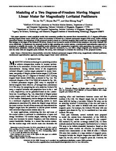
The two degrees of om controller is i mplemented via the {R;G,H} controller as seen in Figure 3. 1, r
( [ rr)u
~~~~G
P
I
Figure 3. 1. S( {R;G,H},P) system. where the interconnected bsystems are completely described by their transfer matrices P (pIm), R (mxq), H (mxp), and G (mxm). Notice that C=[, CrJ G[-H,R]. in a rough sene, we have t matnx equatios with three nknos (R,G,H). In most control problems the dimensons are such that there is freedom i the choice of ., G, and H. In this section it wil be seen that a systematic implementation requres the specification of another matrix parameter. First, examine the conditions imposed on G, H, and R due to the internal stability requirement.
used to
tune" the command/output map. These comments suggest that the additional parameter that needs to be introduced should be one that characterizes the "control action" that needs to be
undertaken by the feedback loop. We can choose either Mf or Xf, since there is a one-to-one relation between them as seen by application of Theorem 2.2 to the systm S({I;G,H},P) which yields the following characterization of maps [Tf] [ 01 rxl [01
it
[Lj
= [D _ + 0 (3.3) where Xf an L are proper and stable maps. Notice that the set of all command/output, command/control and sensitivity matrices is the same in (2.5) and (3.3). It will be seen, however, that not all admissible (T,M,S) can be implemelnted with the {I;G,H} contro1ler. Suppose Xf is chosen, hence Tf=NXf and Mf=DXf are specified. Then the following theorem can be used to synthesize G, R, and H.
TxroE.o -3.1. The system S({R;G,H},P) is intermaly stable if and ony if (i) The control law u=-GHy interally stabilizes P with no nght half plane pole cancellations in the product Gil. (ii) The product GR is such that M=(I+GHP)-'GR satisfies D-IM=X, a stable transfer matrix, where R is stable, GH satisfies (i), and P=ND-1 is coprime. Theorem 3.1 is a direct application of Theorem 2.1. Note that the poles of R and any poles that cancel in the product GH are closed-oop eigenvalues; hence, they must be in the open left half of the complex plane. Second. if the {R;G,H} controller satisfies the internal stability conditions, then the folowing theorem
TNEOlEm 3.2. The st of all the internally stabilizing {R;G,H} controllers that implements the triple (T,M,S) is G = (I-QP)-1Mf, Mf[H R =[Q, M], (3.4) where[Mf,M] = DfXf, Xl with Xf, and X stable; Q=CAI+PCY)I, D-'{Q, (I-QP)] stable, II-.QPI#0; R Stable and nO rght ha plane pole cancellations in GH.
271 Authorized licensed use limited to: UNIVERSITY NOTRE DAME. Downloaded on August 27, 2009 at 15:04 from IEEE Xplore. Restrictions apply.
addition this configuration has two very restrictive conditions: Cr must be stable, and C should be stable (to avoid introducing unnecessary nglt half plane zeros
The first equation in (3.4) establishes a one-to-one relation between G and Mf. The second equation in (3.4) is a model matching type relation and can also be written as Xf[H, R]=[L, X].
in T).
Wv. Concusion
SPECIAL CASES It has been demonstrated that any triple (T,M,S) satisfying the admissibility conditions in Theorem 2.2 can be realized via {R;G,H} compensation. In addition, the set of maps attainable with {I;G,H} compensation is the same. This appears to indicate that any realizable triple (T,M,S) can be implemented via {I;G,H} compensation. However, that is not the case even though {I;G,H} is a two dees of freedom controller. In this section we consider thee two degrees of freedom configuations that are a subset of the {R;G,Hl} controller and show that they may introduce some undesirable limitations.
It has been shown that any realizable triple (T,M,S) can be implemented via {R;G,H} compensation. However, when R or G or H are set to identity, the resulting "two degrees of freedom" controller may not realize the desirable triple because it cannot attain independently the respone and feedback properties. E ples demonstrating this limitations will be presented at the conference.
[1] I.M Horowitz, Synthesis of Feedbak Systems, New York: Academic Press, 1963. [2] D.C Youla and J.J. Bongiorno, "A Feedback
Case 1. {I;G,H} Controller. In this case R=I, which makes M=Mf and L=XH. Substituting the latter equality in the trade off relation in (2-6) gives (3.5) S + NXH =I, 3.6) S + TH = L or This shows that under some conditions this two degrees of freedom" controller cannot achieve independent output distubance rejection and The independent cmmnnd/output response. specification of these maps is stiU possible, for example, when m=q and X is invertible, then let H=X-¶H, which would introduce stable hidden modes. Its efct could be study using [18]. In order to avoid the introduction of unnecessary right half plane- zeros in T, G should be designed to have no right half plane zeros and H should be stable. An extreme case of this fact was given in an example in [2, p.655] which it is put in our terms below. Example 2. Consider {I;G,H} compensation and suppose that the design parameter X is such that it has a finite transmission zero in C+, the right half plane. For this case Cy=GH and Cr=G, and if K and X have been determined then using (2.1) leads to G=(xr-KS)-iX and GH (xr-KN)-i(x2+Kfli). Suppose that (xr-KSI) and (x-KI)l) do not have as a zero the transmisson zero of X in C, then this zero of X must be a zero of G and a pole of H, becoming an unstable hidden mode of the compensated system and the internal stability requirement is not met. Note that if (xr-KRl) has the zero of X in C, in a way that it cancels when foming G, and that (x2+Kfli) does not have it, then H would have it as a pole and internal stability would be maintained. 0 Case 2. {R;G,I} Controller. In this case H=I which makes X=LR and the trade off equation in (2.6) becomes (3.7) T = (I - S)R, showing that indepedt command/output and noise attenuatfon is not possible. Another limitation is that Cy should not have right half plane zeros; otherwise, unnecessary right half plane zeros are introduced in T.
[3]
[4]
Theory of Two-Der-Freedom Optimal Wiener-Hopf Design, IEEE Transactions on Automatic Control. Vol. AC-30, pp. 652-665, July 1985. O.R. Gonz&lez, Analysis and Synthesis of Two Degree of Freedom Control Systems, Ph.D. Dissertation, University of Notre Dame, 1987. J.G. Truxal, Automatic FeedbXa Control System nthis, New York: McGraw Hill,
1955.
[5] K.J. Astr6m, "Robustness of a Design Method [6] [71 [8]
Based on Assignment of Poles and Zeros, IEEE Transactions on Automatic Control, Vol. AC-25, pp. 588-591, 1980. W.A. Wolovich, Linear Multivariable Systems, New York: Spnager-Verlag, 1974. C.T. Chen and S-Y Zhang, IVarous Implementations of Implementable Transfer Matrices," IEEE Transactions on Automatic Control, Vo.L AC-30, pp. 1115-1118, November 1985. M. Vidyasagar, Control Sstem Synthesis: A
Factorisation
Approach,
Cambridge,
Massahusetts: MIT Press, 1985. [91 C.A. Desor and C.L. Gustafson, "Alebraic Theory of Lhnear Multivariable Systems, IS&
L10] [11, [12]
[131
Case43. {R;I,H} ControUer. In this case G=1 which makes Mf=(I-QP) and the trade off equation in (2.7) becomes (3.8) Si= Mf =DXf, (3.9) SR= X or showing that command/output and input disturbance reiection may not be achieved independently. In
[14]
Transactions on Automatic Control. Vol. AC-29, pp. 909 917, October 1984. L. Pernebo, "An Algebraic Theory for the Desig of Controllers for Linear Multivariable SystemsPart I, II," IEEE Transactions on Automatic Control, Vol. AC-26, pp. 171-194, February, 1981. C.A Desoer and C.A. Lin, "A Comparative Study of Linear and Nonlia MIMO Feedback Configurations," International JouMral of SEium.-Siena Vol. 16, , pp. 789 813, 1985. P. J. Antsaklis and M. K. PSa, "Feedback i with -Two Degrees of Freedom: Synthes {G,H;PI Controller,n Proceeding of the 9th World cnes of the International Federation of Automatic Control. Budapest, Hungary, pp. 5-10, July 1984. M. K. Sain and J. L. Peczkowsld,Y"An Approach to Robust Nonlinear Control Design," Proeedins f the 20th_Joint Automatic Control Conference, Paper FA3D, June 1981. T. Sugie and T. Yoshikawa, "General Solution of Robust Tracking Problem in Two-Degree-ofFreedom Control Sytems, IEEE Transactions on Automatic Control, Vol. AC-31, pp. 552454, June 1986.
272 Authorized licensed use limited to: UNIVERSITY NOTRE DAME. Downloaded on August 27, 2009 at 15:04 from IEEE Xplore. Restrictions apply.
[15]
[16]
[17] [18]
[19]
[20]
[21] [22]
[23]
[24]
G. Meyer, "The Design of Exact Non-Linear Model Followers," Proci ofthe 19th Joint Automatic Control Conference, 1980. 0. R. Gonzilez and P. J. Antsalis, "Hidden Modes in Two Derees of Freedom Design: {R;G,H} Controller, Proceedings f the 25th Conference on Decision and Control, pp. 703-704, December, 1986. 0. R. GonzAlez and P. 3. Antsaklis, "EHidden Modes of Interconnected Systems i Control Design Proceedings of the 27th Conference on Decision d Control, pp. , December, 1988. 0. R. GonzAlez and P. J. Antsaklis, ItHidden Modes of Two Degrees of Freedom Systems in Control Design," submitted to the IEEE Transactions of Automatic Control. P. J. Antsaklis, "On Finite and Infinite Zeros in the Model Matching Problem," PragLof the 25th C erenceo Decision and Control, pp. December, 1988. M.K. Sai, B.F. Wyman, R.R. Gejj, P.J. Antsaklis, and J.L. Peczkowski, 'The Total Synthesis Problem of Linear Multivariable Control, Part I: Nominal Design,"Prggdig Of the 20th Joint Automatic Control Confeenr, Paper WP-4A, June 1981. J. S. Freudenberg and D. P. Looze, Freauency Domain ProDerties of Scalr and Multivariabl Feedback SysteMs, Lecture Notes in Control and Information Sciences, Vol. 104, Berlin: SpngeVeriag, 1988. W. A. Woloinch, P.J. Antsaklis, and H. Elliott, "On the Stability of Solutions to Minimal and Nonminimal Design Problems," IEE Tr astions on Automatic_ Control, Vol. AC-22, pp. 88-4, February, 1977. V.H.L. Cheng and C.A. Desoer, "Limitations of the Closed-toop Transfer Function Due to Right-Half Plane Transmission Zeros of the Plant,"i IEEE Transaions on Automatic Control, Vol. AC-25, pp. 1218-1220, December, 1980. M.G. Safonov, A,J. Laub, and G.L. Hartmann, "Feedback. Properties of Multivariable Systems: The Role and Use of the Return Difference Matrix," IEEE Transions on Automatic Control, Vol. AC-26, pp. 514-515, February, 1981.
273 Authorized licensed use limited to: UNIVERSITY NOTRE DAME. Downloaded on August 27, 2009 at 15:04 from IEEE Xplore. Restrictions apply.