Implementing Haptic Feedback Environments from High-level Descriptions ∗ Angela Yun Zhu, Jun Inoue, Marisa Linnea Peralta, Walid Taha Department of Computer Science, Rice University Houston, TX 77005, USA angela.zhu, jun.inoue, mlp3,
[email protected] Marcia K. O’Malley, Dane Powell Department of Mechanical Engineering and Materials Science Rice University, Houston, TX 77005, USA omalleym,
[email protected]
Abstract Haptic feedback can be a critical component of virtual environments used in cognitive research, rehabilitation, military training, and entertainment. A limiting factor in the innovation and the acceptance of virtual environments with haptic feedback is the time and cost required to build them. This paper presents a development environment called iAcumen that supports a new approach for programming such systems. This approach allows the developer to directly express physical equations describing the underlying dynamics. By raising the level of abstraction for the developer, we avoid many of the problems that limit the effectiveness of traditional approaches.
1
Introduction
Haptic feedback systems are an important class of virtual environments. Haptic feedback is force feedback in a human-computer interface [22], relaying realistic tangible sensations to a user. In a virtual environment, haptic feedback augments visual feedback to allow the user to push, pull, feel, and manipulate virtual objects. The application of haptic interfaces in areas such as computer aided design and manufacturing (CAD/CAM), design prototyping, and production evaluation allows users to interact with and visualize virtual objects before manufacturing them. Along the same lines, the users of simulators for training in surgical procedures, control panel operations, and hostile work envi∗ This
research was sponsored by the NSF under Award 0439017, 0720857, and 0747431. Views and conclusions contained in this document are those of the authors and should not be interpreted as representing the official policies, either expressed or implied, of NSF, or the U.S. government.
ronments benefit from increased sensations of realism in the virtual environment that provides force feedback. The haptic display, or force-reflecting interface, is the device that allows the user to interact with a virtual environment. The haptic interface consists of a real-time simulation of a virtual environment and a manipulator, which serves as the interface between the human operator and the simulation. Today, the vast majority of the programming needed to make a haptic system operational is carried out using ad hoc methods, and in systems-programming languages such as C++. This approach has at least two shortcomings. First, for the resulting system to be reliable or efficient, advanced C++ expertise is generally needed. This is a burdensome requirement to place on the developers of such a system, be they engineers or students. Second, the development time using ad hoc approaches tends to be significant, slowing research and innovation that depends on having a functioning haptic system by sometimes months or more. This dependence on expert developers is easier to envision when we look closely at what is involved in programming such systems. Here are some examples: 1. Device interfacing involves building a layer of software on top of device drivers to carry out digital-toanalog and analog-to-digital conversions. 2. Modeling device kinematics generally requires introducing the various appropriate abstractions for representing the human user, coupled via the haptic device, in the virtual environment. 3. Simulation infrastructure involves multi-threading for haptic and graphic rendering loops, and is devicespecific. While generic simulation infrastructure often exists, it is often the case that there is no guarantee on the physical fidelity of such generic engines.
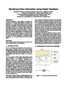
Figure 1. The iAcumen Environment interface for interaction between user and virtual environment allows conceptually clear access to the lowlevel codes needed to inject these external devices into the real virtual world.
In essence, simple simulation engines are built from scratch to ensure their conceptual soundness. 4. Virtual environment modeling is required to simulate the kinematic and dynamic behavior of the desired virtual system or scene, and to track interactions between the human and the objects in the environment.
4. Real-time simulation. In iAcumen, high-level parameters are used to specify the speed of the simulation. This specification becomes part of the specification of the virtual environment.
While some libraries and simulation engines such as CHAI (Computer Haptic Active Interface) 3D [5] are now available, even the most basic offerings require substantial knowledge of C++ for industrial or research grade use. Tools such as MATLAB and Simulink offer a potentially higher level interface to modeling dynamics, but are generally too slow and often not expressive enough to describe dynamics succinctly. With such tools, development of graphics to accompany the haptic simulation still poses a significant amount of labor.
The system is realized by a series of automatic transformations that convert the high-level descriptions into a form that is directly machine executable, and a compilation process is used for converting control algorithms written in RIDL to executable form (Section 3). To illustrate the approach, we present the complete descriptions of the codes needed to realize two haptic tasks that have been used elsewhere in the literature (Section 4).
1.1
2
Contributions
This paper presents an approach to programming haptic systems that avoids these problems. The centerpiece of our approach is a development environment called interactive Acumen, or iAcumen for short (Section 2). The key features of this environment include high-level mechanisms for implementing a virtual environment by describing:
The iAcumen Environment
A physical system with haptic feedback usually has three parts: continuous behaviors, discrete events, and haptic devices. Building such a system requires significant time and effort. To ease this building process, we propose iAcumen, which allows developers to realize such environments in a declarative way.
1. The physical dynamics of virtual objects. The physical description language, PhyDL, allows us to directly describe dynamic equations governing the system being modeled.
2.1
Overview
The iAcumen environment has three components (Figure 1). PhyDL is used to describe continuous behaviors in the system, and RIDL is used to describe discrete events. A PhyDL program directly captures the physical equations describing the underlying system dynamics. A RIDL program specifies system responses (control actions) to events. External modules are used for interactive input and output such as haptic feedback and object positions in the system.
2. Events and their interaction with virtual objects. Modeling of discrete events and control algorithms uses the reactive/interrupt description language, RIDL, in an event-driven programming paradigm. 3. Coupling with external devices, including haptic devices, visual tools, and other application codes. An 2
In the rest of this section, we first show by a simple example what an iAcumen program looks like. Then we use this example to give a detailed explanation of iAcumen’s language components. The syntax of PhyDL and RIDL languages can be found in the Appendix.
2.2
and spring constant k are defined as constants which represent the physical parameters of the simulated system. System dynamics are defined in the same form as equation (1). The line (x,y)=p defines x and y as the x-value and yvalue, respectively, of the ball’s position p. The boundary section specifies the initial position p(0) of the ball and its initial speed p’(0). In this example we have the ball starting at position (20,5) with an initial velocity of (0,0). The external GUI section specifies system output to the user. The output is the position of the ball p as a function of time, and the user can observe the movement of the ball on the GUI. User input can also be declared in this section, where we use keyword reads instead of writes followed by a list of input variable names. The external ridl section describes the communication between PhyDL code and RIDL code. Keywords reads and writes are followed by lists of variables that are read and written by RIDL respectively. Keyword observes event is followed by an event name and the rate of the occurrence of the event. We will explain how these declarations are used in a RIDL program in next subsection. Finally, the simulation section defines the starting time and ending time of the simulation, as well as the step size used by iAcumen’s numerical solver.
A Simple Example
The diagram in Figure 2 shows a simple example illustrating the basic features of iAcumen. A ball is attached to a spring, and the other end of the spring is attached to the origin. Without loss of generality, we assume the original position of the spring is at the origin, and the natural length of the spring is zero. The effects of gravity of the ball are omitted. The dynamics of the system are then defined by the following equation: m ∗ p00 + k ∗ p = (0, 0); (1) Suppose the ball is initially placed at position p = (20, 5). We wish to track the number of times the ball crosses the y-axis (moving from the positive x-plane to the negative x-plane). The iAcumen program to model this system and task is shown in figure 2. On the left is PhyDL code for the virtual system’s dynamics and on the right is RIDL code for the controller to count the number of crosses. Interactions between system and controller are described as part of PhyDL code in the external ridl section. The external GUI section describes interactive input and output of the system.
2.4
The RIDL code of Figure 2 defines three variables, namely cur, prev and crosses. We call these variables reactive behaviors or simply behaviors since they model system behaviors which respond to events. Every reactive behavior has an initial value, which is the value after keyword init, and a set of event handlers in a pair of brackets after keyword in. An event handler has form A=>B, where A is an event name and B is an expression used to update the behavior value when event A happens. Event handlers with keyword later will update behavior value after event handlers without the keyword later. Thus, for example, when event clock happens, behavior cur and crosses will update their values before behavior prev. Temporary names can be used for a behavior if its event handlers will refer to the behavior’s own value. For example, crosses is referred to as a in its own event handler. Event clock and variable x were defined in the external ridl section of PhyDL program. Event clock has rate 0.1, which means it happens every 0.1 seconds. When event clock occurs, any reactive behavior which has an event handler for event clock will update its value. For example, cur gets the current value of x from PhyDL whereas prev keeps the previous value of x until all other updates are completed. The delayed update for
Figure 2. Example: Ball on a spring
2.3
RIDL Code
PhyDL Code
Beginning with the text at the bottom of the PhyDL code, the system section describes system equations. Mass m 3
x(n) = f (t, x, x0 , . . . , x(n−1) )
prev is a result of later annotation. Behavior crosses checks whether the x value is going from a positive value to non-positive. If so, its value is incremented, otherwise it keeps its previous value. RIDL specifies system behaviors that are reactive to system events. This specification provides a natural way to describe controllers. A controller gets feedback from the system being controlled and sends out control signals only when certain events happen. This is different from continuous time system dynamics described in PhyDL. That is why we have two language components in iAcumen.
2.5
We transform the above equation to a set of first order differential equations involving another set of functions u1 (t), u2 (t), . . . , un (t) as u01 u02 u0n−1 u0n
un f (t, u1 , u2 , . . . , un )
m ∗ p00 + k ∗ p = 0
External Modules
would be rewritten into p00 = −k/m ∗ p and then transformed to p01 = p2 p02 = −k/m ∗ p1 , which are first order differential equations. Step 2. Topological Sorting. A set of physical equations usually involves three types of variables: constant and input variables, dynamic variables, and algebraic variables. Dynamic variables are those whose derivatives appear in the model. Algebraic variables are those whose derivatives do not appear in the model, but their values depend on some dynamic variables. We would like to apply numerical methods to the smallest possible ordinary differential equations and compute the values of all other variables as constants or from the solution of this minimal problem set. This is achieved by the following procedure:
Implementation
We implement the virtual environment described in iAcumen by automatically transforming these high-level descriptions into executable C code. This section explains how this is done.
3.1
u2 u3
where ui (t) is equal to the (i − 1)-th derivative of x(t) [1]. For example, the equation
Users interact with a virtual environment through physical devices, some of which can be haptic. Physical devices create a closed loop between the user and the virtual environment. Continuous time position and force signals are exchanged between user and haptic device. Discrete-time position and force signals are exchanged between the haptic device and virtual environment. Our environment provides an interface for interactive input and output. In the PhyDL language we have an external GUI section, where one specifies variables of discrete signals whose values are passed between iAcumen and the external device. We use a pointing device for user input as positions and a visual display for 2-D animations.
3
= = ... = =
• We construct a graph whose nodes are the equations and variables of the problem. • For each equation node, we add an edge between that node and each variable that occurs in the equation. • We use Tarjan’s strongly connected components algorithm [24] to sort the equations and find the strongly connected components.
Compilation of PhyDL
The core of the PhyDL code is a set of differential equations. Numerical methods exist to solve first order differential equations on a digital computer [3, 14]. In PhyDL, we allow differential equations with arbitrary order to be written directly, and the user does not need to worry about the computation order of the input equations. Thus, key tasks in compiling PhyDL are to reduce the order of any differential equation to one, to sort out the topological order among all the equations according to their data-flow dependencies, and to discretize the differential equations using numerical methods.
For example, for the following set of equations m
=
1
(2)
p0 y
= m∗p = 5∗p
(3) (4)
we get the following graph:
Step 1. Order Reduction. A function x(t) satisfying an ordinary differential equation of order n can be written as the n-th derivative of x(t) connected with lower order derivatives by the relation
The graph has three equation nodes and three variable nodes, with the edges between them as on the left of above 4
4.1
graph. Strongly connected components are shown on the right of the graph. We then compute the value of m as a constant, and compute p by solving the differential equation (3). The value of y is computed from the value of p.
The Two-ball Task
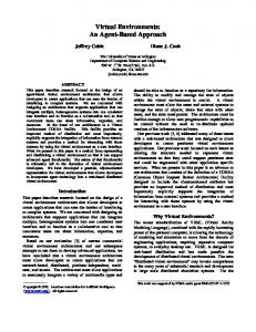
The first task we consider is a task that has been used extensively in haptics research [16]. It uses a pointing device as an input position to control a pair of balls in a virtual environment. The two balls are connected by a spring and damper in parallel, as shown in Figure 3. The white ball is a massless controller, and the black ball is a follower. The effect of gravity on the black ball is neglected, as the system is assumed to be acting in a horizontal plane. The user operates the pointing device to control the white ball. The output is the position of the black ball and the force feedback to the user. We display the positions of both balls on the GUI and the appropriate force feedback is sent to a haptic device. A snapshot of the GUI with this task running in iAcumen is shown in Figure 4.
Step 3. Discretization. Discretization transforms continuous differential equations into discrete time difference equations. Different numerical methods can be applied in this process. Currently, three numerical solvers are implemented in iAcumen. They use the Euler [3], RK4 [14] and BS3 [2] methods. The step size of the solver is defined in the simulation section. Using the Euler method as an example, the discretization is carried out as follows. Assume that f (t, x) is continuous in the variable x, and consider the differential equation x0 = f (t, x) with x(a) = x0 , over the interval a ≤ t ≤ b. Euler’s method uses the formulas tk+1 = tk + h, and xk+1 = xk + h · f (tk , xk ) for k = 0, 1, 2, ..., m−1 as an approximate solution to the differential equation using the discrete set of points {tk , xk }k∈0···(m−1) , with t0 = a and h = tk+1 − tk .
3.2
Compilation of RIDL
The RIDL code is a set of event handlers. The compilation of RIDL takes this set of event handlers and transforms them into a C-like language. For example, the RIDL code on the right side of Figure 2 would be transformed to:
Figure 3. The Two-ball Problem The dynamics of this system are defined as follows: F k F b F F
cur=0; prev=0; a=0; crosses=0; if clock happens {cur = x; if cur0 then a=a+1 else (); crosses=a; prev=x;}
= = = =
k ∗ (white ball − black ball); b ∗ (white ball0 − black ball0 ); F k + F b; m ∗ black ball00 ;
The PhyDL code for this system is as follows: The generated code has a set of variable declarations followed by a set of if statements. Initial values of the variables are the same as declared in RIDL code. Each if statement corresponds to an event. Inside an if statement, the first part of the code is generated from event handlers without later notation, and the second part of the code is generated from event handlers with later notation in original RIDL code. The computation order in each part is decided by the data-flow dependencies between the variables. Details of RIDL compilation can be found in [15].
4
boundary black_ball with black_ball(0) = (0,0), black_ball’(0) = (0,0); system F_k = k * (white_ball - black_ball); F_b = b * (white_ball’ - black_ball’); F = F_k + F_b; F = m2*black_ball’’; k = 4; b = 1; m = 1;
In addition to the dynamics above, this task also introduces two boxes. The user’s objective is to control the black ball to cross these two boxes alternately by manipulating only the white ball and leveraging the dynamics of the two-ball system. The white ball is controlled by a pointing device, which acquires real time input from the user. The positions of the boxes are specified in PhyDL as follows:
Examples
This section presents implementations of two different tasks in iAcumen.
box1 = (350, -300);
5
box2 = (-350, 200);
where box1 and box2 define the bottom-left points of the two boxes. The default size of the boxes is 50 for each side. The counting of the crosses is implemented in RIDL as follows: cur = init 0 in {clock => black_ball}, prev= init 0 in {clock => black_ball later},
We first define variables cur and prev, each of which has initial value zero. When event clock happens, cur and prev update their values to the current and previous value of black ball respectively. cross1 = init a=0 in {clock => if (cur in box1) && !(prev in box1) then x+1 else x} cross2 = init a=0 in {clock => if (cur in box2) && !(prev in box2) then x+1 else x}
Figure 5. The Inverted Pendulum Problem F
Then variables cross1 and cross2 are defined. Behavior cross1 checks whether the black ball has just gone into box1 from outside when event clock happens. If so, the value of cross1 is increased by one. Behavior cross2 is defined similarly.
0
(M + m) ∗ x00 + m ∗ l ∗ (a00 ∗ cos(a) −a0 ∗ a0 ∗ sin(a)); = m ∗ l ∗ (−g ∗ sin(a) + x00 ∗ cos(a) + l ∗ a00 );
=
The PhyDL code implementing the equations is as follows: boundary a with a(0) = 0.1, a’(0) = 0; system F = (M+m)*x’’ + m*l*(a’’*cos(a) - a’*a’*sin(a)); 0 = m*l*(-g*sin(a)+x’’*cos(a)+l*a’’); cart = (x, y); M = 10; m = 1; l = 4; ball = cart + rotate((0, l), a);
This is the complete iAcumen specification for the dynamics of this task. The visual and haptic specification are similar to the first example. Figure 4. Visual Display for Two-Ball Task
5 4.2
An Inverted Pendulum Task
Related Work
The iAcumen environment has some similarities to Problem Solving Environments (PSEs) [12, 21], such as helping the user express equations directly. Also, in iAcumen, we have a real-time siler, which does seem typical for PSEs. However, iAcumen also has some significant differences. It does not try to expose the differential equation solution techniques to the user, and in fact iAcumen tries to hide such details from the user. Several commercial tools are currently available for modeling physical systems and building virtual environments. Each has its strength in some specific area, or be powerful to some extent, but each also has disadvantages that limit its applicability for modeling virtual environments with haptic feedback. Solidworks [19, 17] and ProEngineer [7] are 3D mechanical CAD programs aimed at design automation and optimization. These tools are widely used by product designers and mechanical engineers for drafting their products. They provide a systematic way for constructing solid objects and
The second task we consider here has been used in control design with haptic feedback as a performance enhancement [6]. The task uses a pointing device as force input to a cart of mass M , on which is placed an inverted pendulum with mass m lumped at the end of a rod of length l (Figure 5). The pendulum is subjected to the effect of gravity, and can rotate freely about the pin joint connecting it to the cart. The cart is externally controlled by the pointing device in the horizontal as if there is a spring connected between the cart and the pointing device. Thus, the distance between the pointing device and the cart on the x-axis generates a spring force F . The purpose of the task is to control the cart to stabilize the position of the pendulum, so that the angle between the rod and vertical remains small. The positions of the cart and the pendulum are visualized on the GUI and force feedback is sent to a haptic device. The dynamics of the system are as follows: 6
sures that the simulation can be carried out within the specified simulation constraints would be invaluable for delivering production-quality applications that are based on iAcumen. We are also very interested in verifying the accuracy of simulations, as well as in providing tools for the automatic analysis of some control-theoretic properties of the virtual systems described in iAcumen. Finally, while this work emerged in the context of developing haptic feedback virtual environments, it appears that there are significant potential applications in the broader domain of virtual environments for this approach. As such, we expect that some of the most exciting future work will be in exploring the range of applications for the iAcumen system.
assemblies. However, Solidworks and ProEngineer only provide limited support for modeling system dynamics and object interactions. For example, system dynamic equations cannot be easily modeled using these tools. In contrast, a number of tools aim at modeling rigid body dynamics of physical systems, such as Open Dynamics Engine (ODE) [18]. These tools are capable of 3D visualization and simulation of pure mechanical systems. However, the modeling of system dynamics and control are not distinguishable from each other in these tools. In addition, significant effort is required to translate from system dynamic equations to programs. Some tools for solving equations have been used for modeling and simulation, such as Mathematica [23], SciLab [13] and MathCAD [20]. In general, using such solutions becomes very clumsy if the virtual environment to be modeled involves both continuous behaviors and discrete events. Additionally, these tools do not provide an interface for interactive user input and output. MATLAB/Simulink [4] is widely used for modeling and simulation. However, it is not always obvious how to derive MATLAB/Simulink code from physical equations. Also, the user needs to have a deep knowledge of MATLAB/Simulink to correctly interpret the result of its simulations. For example, MATLAB lacks a package system, all functions share the same global name space, and function precedence depends on the user’s MATLAB path, all of which make it possible for the same input to give different results for different runs. Modelica is an equation-based, object-oriented language for modeling physical systems [8, 10]. Physical equations can also be easily transferred into a Modelica program. Modelica is a specification language only and thus requires an external computational environment to actually simulate system response. A limited number of computational environments support Modelica simulation, such as OpenModelica [9], Dymola [10], and MathModelica [11]. All of these environments have complex compilation processes and demand the user to have a profound understanding of Modelica semantics. A more detailed discussion of these environments and their drawbacks can be found in [25].
6
References [1] O. Aberth. Introduction to Precise Numerical Methods, Second Edition. Academic Press, Inc., Orlando, FL, USA, 2007. [2] R. W. Brankin, I. Gladwell, and L. F. Shampine. RKSUITE: A Suite of Explicit Runge-Kutta Codes. In Contributions in Numerical Mathematics, pages 41– 53. World, 1993. [3] J. C. Butcher. The Numerical Analysis of Ordinary Differential Equations. Wiley, 1987. [4] A. Cavallo, R. Setola, and F. Vasca. Using MATLAB, SIMULINK and Control System Toolbox: A Practical Approach. Prentice-Hall, Inc., Upper Saddle River, NJ, USA, 1996. [5] CHAI. http://www.chai3d.org/. [6] H. Ching, L. Xie, J. Mao, R. Duo, and C Kong. Teleoperation of Inverted Pendulum using Wave Variables in the Framework of Reflection Coefficient. In SICE Annual Conference, pages 716–721, 2008. [7] S. S. Condoor. Mechanical Design Modeling Using ProEngineer. McGraw-Hill, Inc., New York, NY, USA, 2001. [8] H. Elmqvist, S.E. Mattsson, D. Ab, and M. Otter. Object-Oriented and Hybrid Modeling in Modelica. In Journal Europ´een des Syst`emes Automatis´es, 2001. [9] P. Fritzson, P. Aronsson, A. Pop, H. Lundvall, K. Nystrom, L. Saldamli, D. Broman, and A. Sandholm. OpenModelica - A Free Open-Source Environment for System Modeling, Simulation, and Teaching. In Computer-Aided Control Systems Design, 2006 IEEE International Symposium, volume 1, pages 1588– 1595, 2006. [10] P. Fritzson and P. Bunus. Modelica, a General ObjectOriented Language for Continuous and DiscreteEvent System Modeling and Simulation. In Proceedings of the 35th Annual Simulation Symposium, pages 14–18. IEEE Press, 2002. [11] P. Fritzson, J. Gunnarsson, and M. Jirstr. MathMod-
Conclusions and Future Work
This paper presented a method for building haptic environments at a higher-level of abstraction. The approach allows us to realize virtual environments directly from physical equations that describe the dynamics of objects in the virtual environment, augmented with very high level specifications of events, event occurrences, and integration with external hardware and software devices. There are several areas where technical advances can be made to iAcumen. For example, a static analysis that en7
[12]
[13] [14] [15]
[16]
[17] [18] [19]
[20]
[21]
[22]
[23]
[24]
[25]
PhyDL syntax The syntax of PhyDL is as follows.
elica - An Extensible Modeling and Simulation Environment with Integrated Graphics and Literate Programming. In Proceedings of the 2nd International Modelica Conference, 2002. E. Gallopoulos, E. Houstis, and J.R. Rice. Computer as thinker/doer: Problem-solving environments for computational science. In IEEE Computational Science & Engineering, volume 1, pages 11–23, 1994. C. Gomez. Engineering and Scientific Computing with SciLab. Birkhauser Boston, 1998. A. Iserles. A First Course in the Numerical Analysis of Differential Equations. Cambridge Univ. Press, 1996. R. Kaiabachev, W. Taha, and A.Y. Zhu. E-FRP with priorities. In EMSOFT ’07: Proceedings of the 7th ACM & IEEE International Conference on Embedded Software, pages 221–230, New York, NY, USA, 2007. A. Ko and J. Choi. A Haptic Interface using a Forcefeedback Joystick. In SICE Annual Conference on Instrumentation, Control and Information Technology, pages 202–207, 2007. D. Murray. Inside Solidworks. Delmar Books, 2000. ODE. http://www.ode.org/. D. C. Planchard and M. P. Planchard. Assembly Modeling with SolidWorks 2008. Schroff Development Corporation, 2008. P.J. Pritchard and R. Pritchard. MathCAD: A Tool for Engineering Problem Solving (B.E.S.T. Series). McGraw-Hill Higher Education, 1998. J.R. Rice and R.F. Boisvert. From scientific software libraries to problem-solving environments. In IEEE Computational Science & Engineering, pages 44–53, 1996. J. K. Salisbury, F. Conti, and F. Barbagli. Haptic Rendering: Introductory Concepts. In IEEE Computer Graphics and Applications, volume 24 (2), pages 24– 32, 2004. P.A. Savory. Using Mathematica to aid simulation analysis. In WSC ’95: Proceedings of the 27th Conference on Winter Simulation, pages 1324–1328, Washington, DC, USA, 1995. IEEE Computer Society. R. Tarjan. Depth-First Search and Linear Graph Algorithms. SIAM Journal on Computing, 1:146–160, 1972. S.A. Vaze, J.E. DeVault, and P. Krishnaswami. Modeling of Hybrid Electromechanical Systems using a Component-based Approach. In IEEE International Conference on Mechatronics and Automation, volume 1, pages 204–209, 2005.
Variable names Variables Constants Elementary operators
x v c f
Logical operators Arith expressions
⊕ d
Boolean expressions b
∈ X ::= x | v 0 ∈ Qn ::= + | − | ∗ | / | sin | cos | power | abs | index | direction | rotate | proj ::= > | = | < | ≥ | ≤ | 6= ::= c | v | f hdi i | if hb, d1 , d2 i | integration (d) ::= d ⊕ d | ¬b | b || b | b &&b
External names Module names Timings
E S T
∈ ∈ ::=
Equations System modules
e m
::= ::=
Modules s Interface commands C
::= ::=
p
::=
PhyDL programs
E ⊇ {ridl, matlab, GUI} S starting time = c ending time = c step size = c d = d | Shxi i [boundary {vi (ci ) = di }] system {ei } module S = (ports {xi } m) reads {vi } | writes {vi } | {[when, rate] t = ci } {si } simulation T {external E {Ci }} m
We use a|b or [a, b] to denote a or b, and use [a] to denote that a is optional (may or may not appear). In constant definition, Q is the set of fractions, or equivalently, floating point numbers. In the definition of arithmetic expression, we write hb, d1 , d2 i to denote a sequence and hdi i to denote a sequence of d’s. We use {ai } to denote a set of a’s. PhyDL has a module system that is not used in the paper. Module system is useful when modeling complicated systems, where several parts of a system have their dynamics described by same equations. For example, a robot with multiple identical legs. The compilation of PhyDL programs with subsystems involves an instantiation step before the compilation steps described in the paper. RIDL syntax The syntax of RIDL is as follows. Note that it refers to some PhyDL definitions introduced above. Event name Passive behaviors Reactive behaviors Event handlers Behaviors RIDL programs
I D R H B P
∈ ::= ::= ::= ::= ::=
I c | x | f hDi i | if hb, D1 , D2 i init [x =]c in {Hi } I ⇒ D [later] D|R {xi = Bi }
Passive behaviors in RIDL are similar to arithmetic expressions in PhyDL, except that derivative and integration operations are not allowed in RIDL syntax. In particular, RIDL handles discrete time events rather than continuous behaviors.
Appendix: Syntax of PhyDL and RIDL This section presents the formal definitions of PhyDL and RIDL syntax. 8