Implementing Partial Persistence in Object-Oriented Languages †
†
†
?
Fr´ed´eric Pluquet , Stefan Langerman , Antoine Marot , and Roel Wuyts †
Universit´e Libre de Bruxelles
{fpluquet,stefan.langerman,amarot}@ulb.ac.be ?
Imec and KULeuven
[email protected] Abstract A partially persistent data structure is a data structure which preserves previous versions of itself when it is modified. General theoretical schemes are known (e.g. the fat node method ) for making any data structure partially persistent. To our knowledge however no general implementation of these theoretical methods exists to date. This paper evaluates different methods to achieve this goal and presents the first working implementation of partial persistence in the object-oriented language Java. Our approach is transparent, i.e., it allows any existing data structures to become persistent without changing its implementation where all previous solutions require an extensive modification of the code by hand. This transparent property is important in view of the large number of algorithmic results that rely on persistence. Our implementation uses aspect-oriented programming, a modularization technique which allows us to instrument the existing code with the needed hooks for the persistence implementation. The implementation is then validated by running benchmarks to analyze both the cost of persistence and of the aspect oriented approach. We also illustrate its applicability by implementing a random binary search tree and making it persistent, and then using the resulting structure to implement a point location data structure in just a few lines. 1 Introduction In the algorithm literature, a gap exists between textual descriptions of algorithms in scientific articles and their implementation in a programming language. Algorithms are described in english text or (pseudo-)code and expressed using three kinds of operations: basic operations (such as basic arithmetic, assignment or simple control-flow), new operations (introduced by the
paper) and external operations (referencing other research). When implementing the algorithm these operations need to be implemented efficiently and easily in a concrete language. This is easy enough for the basic operations that are supported directly in almost any programming language in use today. New operations are typically described in detail by the author of the proposed algorithm, and therefore can be implemented with some more work. But problems can arise with the external operations because they potentially hide very complex implementations not explained in the same article (referencing previous articles), thereby posing a real problem for developers. An example of a well-understood yet complex algorithm frequently encountered is that of persistence. A regular data structure is ephemeral, i.e., only the last state of the data structure is stored and previous values are lost. On the other hand, a persistent data structure keeps old values when an update operation is performed. Several flavors of persistence were defined by Driscoll, Sarnak, Sleator and Tarjan[15]. A structure is partially persistent if previous versions remain accessible for queries but not for updates. A fully persistent structure offers accesses to its previous versions for queries and updates, where each update operation on a version of the data structure creates a new branch from this version for the new version. Different methods presented by Driscoll et al.[15] can be used to make ephemeral structures persistent with only a constant factor slowdown. However, their most efficient techniques can only be applied in a pointer model, i.e., when data structures are only composed of a network of records of bounded size and in-degree. Their less efficient fat node method can be applied in the RAM model to obtain partially persistent data structures with
37 Copyright © by SIAM. Unauthorized reproduction of this article is prohibited
a O(log m)1 slowdown in speed (where m is the number of updates on the structure). Using the fact that version numbers are integers between 0 and m, one can use YFast trees of Willard [33] combined with the dynamic perfect hashing scheme of Dietzfelbinger et al.[13] to obtain partially persistent arrays (or persistence in the RAM model) with a slowdown of O(log log m) in speed. This result was extended to full persistence by Dietz[12]. Note that all the above results are theoretical, and to our knowledge, no general and fully transparent persistent system has been implemented to this day. By transparent (or non intrusive), we mean that no modification must be done to the code implementing an ephemeral structure to transform it into a persistent one. However, a quick review of the literature reveals that over 20 papers use persistence as an external operation [5, 34, 17, 18, 1, 20, 3, 6, 21, 10, 25, 22, 2, 32, 23, 9, 16, 8, 7, 4, 11], notified by the simple sentence “Make this structure persistent” or “The time and space bounds can be reduced if persistent structures are used”. Given that no implementation of a mechanism is available to make a structure persistent, implementing either of these more advanced results is very difficult and time-consuming. Two partial solutions were previously proposed to introduce the Driscoll et al. persistence as an external operation. The first one is the Zhiqing Liu persistent runtime system [24]. The entire system is persistent and uses a persistent stack and persistent heap to save changes. The granularity of changes to be recorded can be tuned to manage the quantity of recorded data. This solution is not flexible enough to change a subset of classes to persistent ones. However, in scientific articles, it is common that only a subset of all used structures for algorithms must be made persistent. The second previously existing solution is the Allen Parrish et al. persistent template class [27]. A template class Per is provided by the author. The author admits that the solution suffers from some problems (e.g. because of references in C++) and it is not transparent for the initial program since all variable declarations must be modified by hand. On the other side all previous practical attempts to save previous states in a general and transparent way lack some of the main advantages of Driscoll et al. efficient persistence: some papers[28, 29] propose techniques to trace a program, events are logged, but full snapshots of previous versions are not readily accessible. Caffeine[19] on the other hand stores previous states as prolog facts for fast future queries, but the snapshots 1 Throughout this article, we write lg 0 = lg 1 = 1 and lg x = log2 x for x ≥ 2.
are taken by brute force, as a copy of the entire set of objects to trace. This paper shows how any ephemeral data structures in an object-oriented language can become partially persistent (i.e., each state of any object can be saved and accessed efficiently in time and space) without modifying the ephemeral program, in a simple, transparent and fine-grained way. To obtain these results we developed a variant of the fat node method proposed in [15] to save previous states in the objects themselves, and tested several data structures optimized for this task. We use aspect-oriented programming to transparently include a mechanism for detecting state changes. Any paper that uses persistence as an external operation therefore becomes much easier to implement. We show this by implementing a treap, a random binary search tree [31] and making it partially persistent in one line. We use persistent treaps to implement the planar point location solution from [14] in just a few lines of code. The rest of this paper is organized as follows. Section 2 introduces the fat node method of Driscoll et al. and discusses some improvements. Section 3 explains how we implement this theoretical method in an object-oriented language. Section 4 shows how to use our system to create a data structure for planar point location using persistent search trees in a few lines of code. Benchmark results of our implementation are described in Section 5. 2 The Fat Node Method 2.1 Fat Node Method in the RAM Model. The fat node method as proposed by Driscoll et al.[15] is used to transform an ephemeral structure into a partially persistent structure in which changes of fields occurring in a node are saved in the node itself without erasing old values of fields. Although the fat node method was originally described only for data structures in the pointer model of computation, we will discuss it in the more general RAM model of computation to which it easily generalizes. In the RAM model of computation, each memory unit has an address and instructions can be used to either read or store a value at some address. Each memory unit is ephemeral by nature, i.e., when an instruction is used to store a new value at some address, the previous value is lost forever. A data structure is composed of a set of memory units containing the data, along with routines (lists of instructions in the RAM model) that are used to perform operations (queries or updates) on the data. In order to transform such a data structure into a partially persistent one, we first need to maintain a global version
38 Copyright © by SIAM. Unauthorized reproduction of this article is prohibited
counter which is incremented every time an operation is performed on the data structure (note that several basic instructions could occur when performing an operation). We then simulate the RAM model by maintaining for every memory unit an auxiliary structure which records the values stored at that address after every operation where it is modified, along with the timestamp (value of the version counter) for the time at which that value was stored. Whenever the original structure performs a store on an address, if the current version counter is present in the auxiliary structure, the corresponding value is updated. Otherwise, a new entry is added in the auxiliary structure, with the new value and the current timestamp. Whenever an instruction wants to read a value from an address at time t, the auxiliary structure is searched to find the value whose timestamp is the largest among those less than t. This way, persistent query operations can be performed at any desired time in the past. A data structure to maintain the auxiliary data structure in O(1) time per update and O(log n) time per search can be developed using standard data structure techniques. The specific data structure we use and optimize for those operations is described in the next subsection. 2.2 An Efficient Structure for States. As described above, the auxiliary structure for each memory address must allow to add a new value with a timestamp greater than all previously stored timestamps, to update the value associated with the most recent timestamp, and to search for the value whose timestamp is the largest among those smaller than a given t. Of course any dictionary data structure that implements predecessor queries would do (e.g., any balanced tree, skip-list, etc.), but since this will be the most heavily used structure after applying the persistence transformation, special care has to be taken to make the structure as efficient as possible while keeping the memory overhead within reasonable bounds. The simple structure we describe stores an extensible array where new elements can be appended at the end in O(1) time (assuming constant time memory allocation), and where the number of pointers to follow and the number of comparisons to be performed during a search are both bounded by lg m + 2 in the worst case where m is the number of elements in the array. The space used is O(m). The structure is composed of a linked list of blg mc + 1 arrays of exponentially decreasing sizes 2blg mc , 2blg mc−1 , . . . , 1. Each array stores (value, version number) pairs in decreasing order of version number, and all arrays are completely filled except maybe
(a) 1 element
(b) 2 elements
(b) 6 elements
(b) 8 elements
Figure 1: Structure to save versions of a field.
the frontmost and largest array. The frontmost array maintains the position of its element with the largest version number. When storing the first value in an empty structure during initialization, an array of size one is created and the value and version number are stored (Fig.2.2 a). When a change occurs a second version is generated, an array of size 2 is created and linked to first array; the new version is stored along with its version number at the end of this array (Fig.2.2 b). Further changes fill the frontmost array from back to front until the array is full. When the array is full and the next update occurs, a new array is created whose size is twice that of the previous array, and is linked to that previous array, and the next version is stored in the last position of the new array (see Fig.2.2 c and d). The last version of the field is stored in the frontmost list and its value can be retrieved or updated in O(1) time. The insertion of a new version costs O(1) time as well. When searching for the entry whose timestamp is the largest among those smaller than t, the list is followed until the array containing the sought element is found. This can be done by comparing t to the first element of each array until the last array is reached or an element larger than t is found. If 1 ≤ k ≤ blg mc pointers are followed, then k comparisons have been made and the array found is of size 2blg mc−k+1 . That array is then binary searched to find the desired element, using blg mc − k + 2 further comparisons. 2.3 Snapshots. Initially we had planned to make persistent objects record all versions of each field, regardless of the specific task at hand, but when implementing this solution we realized that different applications could need different granularities of versioning information, and that it is usually not necessary to save all states all the time. Suppose for example that we want to implement a balanced tree in the persistent language. If the application only requires to go back to previous consistent states of the tree, the interme-
39 Copyright © by SIAM. Unauthorized reproduction of this article is prohibited
diate state changes during the balancing operations do not need to be stored. On the other hand, if we want to use persistence to debug an operation in the same tree, it could be useful to store all steps. We therefore need a way for the user to indicate the consistent states in a system or, in other words, to define the granularity of the persistence. The solution we decided to implement allows the user to explicitly indicate when the states have to be remembered by taking a snapshot, which can be done anytime. The result of a snapshot is a picture of the complete system at the time when it is created. To the user it is an object that can be used to access any data at the moment the snapshot was taken. In our previous example, the user is interested in seeing consistent states of a tree, would only take snapshots before or after performing operations on the tree (add, delete, . . . ), while a debugger application would take snapshots after any change to any tree object. In practice, when the user takes a snapshot, the implementation will return an object containing the global version number, and will increment the global version number. Then, whenever the value of a field f is changed, if the version number of the last saved state of f is equal to the global version number, the value of the last state can be forgotten and replaced by the new value. Otherwise, a new state is created with the global version number as version number. The global view mechanism is used to browse past states. At each read of an attribute of a persistent object the system checks if the global view is activated or not. If not (the system is at now), the original read is performed. Otherwise the system looks for, in the states structure associated to this attribute, the last value before or at version number joined to the global view. Using a persistent object in the past is completely transparent for the user: he chooses a previously taken snapshot and manipulates objects as he could in the present. Because we implement partial persistence, a change in past is not permitted (only querying the structure is allowed). 3 Implementation 3.1 Possible Choices. The easiest way to use persistence could be to select a language that already persistent. For instance, in a functional language all data structures are intrinsically persistent [26]. However few algorithms are developed in a functional model and their analysis is often difficult. Because most algorithms are described using imperative models of computation we restrict our research to this paradigm. Unfortunately, to our knowledge, no usual imperative language (e.g. C++, Java, . . . ) allows to imple-
ment directly the persistence in a transparent way: an instrumentation of all accesses to given variables must be performed, without modifying original code. So we must interfere in the compilation process. We see several possible methods to insert a persistence mechanism in a transparent way for imperative languages: before the compilation (pre-compilation), after the compilation (change the bytecode), during the compilation and add more reflection to languages. Before the compilation Adding transparent persistence via a pre-compilation would offer the advantage of being able to add the same pre-compiler to any implementation of the language. However, it requires to parse the code and extract necessary information to perform a transformation of the code. These operations are non-trivial. After the compilation The manipulation can be also performed on the bytecode generated by a compiler. In that case, any language that can be transformed into the same bytecode could be rendered persistent. However, manipulating bytecode is also a complex task and it is not clear how one would instruct the persistence system on which parts of the code should be rendered persistent. During the compilation More generally, one could interact at any level of the compilation (lexical analysis, parsing, semantic analysis, generation of code and optimization of generated code). The compiler must provide enough flexibility to accept this kind of interaction (either directly in the source code if it is open-source or via a plugin mechanism). Adding more reflection Some solutions exist that add more reflection and introspection at a high abstraction level to instrument accesses to variables in existing languages. Aspect-Oriented Programming (AOP) has been developed in this way. Having that type of mechanisms at hand greatly simplifies the transparent implementation of persistence. To develop our solution we selected the widespread object-oriented imperative programming language Java with the AspectJ module for the AOP functionalities. Note that our solution is easily adaptable to any language supporting the aspect paradigm (e.g. C++,C#, Python, Smalltalk), a Smalltalk implementation following similar principles was developed in parallel to the Java system described here. 3.2 Aspect-Oriented Programming. Aspectoriented programming (AOP) is a modularization mechanism that allows a program to be split between
40 Copyright © by SIAM. Unauthorized reproduction of this article is prohibited
(functional) base code, and so called cross-cutting behavior that needs to be applied throughout the base code. Take for example an application that implements a number of data structures (vectors, balanced trees, ...). For helping with debugging, the developers want to keep a log file that shows whenever elements are deleted from these data structures. A good solution to implement this behavior using a non-AOP language would be to implement a logging facility, and to change the delete functionality in the data structure implementations to call this logging facility. An alternative would be to call the logging facility in the code that uses the data structures. In both cases however, the logging code that is only there for the purpose of debugging is added to the base program (either in the data structures themselves or in the code that uses the data structures). Using aspect-oriented programming, the data structures and the client code are written without taking the logging code into account. The logging code is implemented in its own module (an aspect), that contains the logging facility itself as well as expressions that indicate where this logging facility needs to be called. The base program and this logging code are then composed by a so-called weaver, that produces the final program that does logging. An aspect implements the behavior that needs to be called, and specifies when the behavior needs to be called. In our example, we could decide to call the log functionality as last statement in the implementation of any delete procedure in any of our data structures (which corresponds to the first manual solution). We could also decide to execute the log functionality after every call to a delete procedure, corresponding to the second solution. An aspect language hands a developer a number of points (join points) in the execution of the program where code can be called (the advice code), and a language to use them. Such language typically supports quantifiers and wildcard expressions that make it easy to specify global criteria. In our example, the second approach needs to express ’After any call to a method named delete, call the following piece of code: ...’. Exactly what join points are offered depends on the aspect language. Typically code can be executed before, after or around the execution of behavior (calling a function, constructing an object, etc.). Aspect languages also offer support to add elements to existing code (e.g., methods, fields, interfaces, if AOP extends OOP). 3.3 Java Specific Implementation Details. In order to implement persistence we must map each field of the object to an instance of our states structure containing the different values of this field. Fields in
Java are statically typed, that is, their type can not be modified during the execution of a program. Thus a states structure can not be stored directly in place of those fields. Furthermore AspectJ only provides the names of the fields accessed. Because of this, we have to create a dictionary in each object for mapping the field name to the structure storing its states (named fieldsAndStates in previous codes). When a field in a persistent object is accessed, a lookup in the corresponding dictionary is performed. 3.4 Transparent Persistence with AspectJ. Our implementation uses the aspect-oriented AspectJ system to add persistence to existing Java programs without having to change these programs. In order to use AspectJ to make classes persistent, the developer writes an aspect declaration. For example, the following AspectJ code makes all classes in a package treap persistent (note the wildcard expression treap.*): declare parents: (treap.*) implements PObject;
Note that other criteria could be used, such as explicitly enumerating classes or selecting a number of classes based on their name. Technically, the aspect declaration updates the existing class to add our PObject interface to it. AspectJ will install all necessary wrappers to classes implementing the PObject interface, adds an instance variable in these classes, initializes them, and finally extends classes with some methods to access old states of fields of instances. Note that this solution is transparent. The existing structure is made persistent with the aspect declaration, which is not part of the ephemeral implementation. The rest of the aspect is used to manage the states: • Adding a new variable to contain a dictionary in each persistent object: public FieldsAndStates PObject.fieldsAndStates = new FieldsWithStates();
• Declaration of the pointcuts of setters and getters of persistent objects, but not in the aspects package: // declaration of pointcut setters with 1 arg pointcut setters(PObject t): // all updates of PObject implementors set(* PObject+.*) // not in ’aspects’ package && ! within(aspects.*) // put the target in the variable t && target(t);
41 Copyright © by SIAM. Unauthorized reproduction of this article is prohibited
is used to locate the region containing the point, also in O(log n) time. Unfortunately, the worst-case space requirement for this structure is Θ(n2 ). To solve this problem, Sarnak and Tarjan[30] use persistence in order • Definition of the advice code after each update of a to reduce the space to O(n). A vertical line sweeps the field of a persistent object (we ask to save the new plane from x = −∞ to x = +∞, maintaining at every point the vertical order of the segment in a balanced value for the set field): binary search tree. The tree is modified every time the after(Object newValue, PObject t) : line sweeps over a point, but all previous versions of setters(t) && args(newValue) { the tree are kept, effectively constructing Dobkin and t.fieldsAndStates.addStateWithValueFor( Lipton’s structure while using a space proportional to // the field name: the number of structural changes in the tree. thisJoinPoint.getSignature().getName(), In order to illustrate how transparent persistence // the new value stored in field: can simplify the implementation of complex data strucnewValue); } tures, we implemented a random treap[31], a randomized binary search tree. The system then transforms • Definition of the advice code around each read on automatically this structure into a partially persistent a field of a persistent object: structure via the persistence aspect. The following code is placed in a class storing a set Object around(PObject t) : getters(t) { of points. Each point stores its incoming and outgoing if(!Snapshot.globalViewActivated()) segments. In the construction of the point location return proceed(t); // original read data structure, each point of the set is swept by the // retrieve the states of the field sweepline, its outgoing segments are added in the treap, OrderedStates states = t.getStatesFor( thisJoinPoint.getSignature().getName()); the incoming are removed and a snapshot is taken and // search the good version of field stored in the info associated to the point. // same for all read operations pointcut getters(PObject t): get(* PObject+.*) && ! within(aspects.*) && target(t);
// in respect to current snapshot VN return Snapshot.valueOfStates(states);}
Note that, because to AspectJ limitations, the arrays can not be made persistent in this way: AspectJ does not offer a mechanism to instrument accesses to the elements of an array. However such a feature is available in the Smalltalk implementation, the reflection mechanism being more powerful. 4 Planar Point Location and Treaps Planar point location is a classical problem in computational geometry: given a subdivision of the plane into polygonal regions (delimited by n segments), construct a data structure such that given a point, the region containing it can be reported quickly. Dobkin and Lipton[14] proposed a solution consisting in subdividing the plane into vertical slabs determined by vertical lines positioned at each vertex. Within each slab, there exists a total order between line segments determined by the order in which any vertical line in the slab intersects them. Each segment is associated to the polygon just above it, and a balanced binary search tree storing the segments is constructed for each slab. When a point is queried, its x-coordinate is used to determine which slab contains it in O(log n) time, and the binary search tree of the corresponding slab
private void constructRTreap(){ rtreap = new RandomTreap(); Iterator it = points.iterator(); while(it.hasNext()){ Point point = (Point)it.next(); LinkedInfosPoint info = point.getInfo(); Iterator segmentsIt = info.incomingSegmentsIterator(); while(segmentsIt.hasNext()){ rtreap.delete((Segment)segmentsIt.next());} segmentsIt = info.outgoingSegmentsIterator(); while(segmentsIt.hasNext()){ rtreap.put((Segment)segmentsIt.next());} info.setSnapshot(Snapshot.takeSnapshot());}}
In the location step of a point p, the slab containing p is determined. The user asks to the system to see the structure through the snapshot associated to the left point of the slab. The treap can then be used normally to locate the point. public Segment locatePoint(Point p){ Point thePoint = getLastPointBefore(p); LinkedInfosPoint assoc = (LinkedInfosPoint) points.get(thePoint); Snapshot.globalViewOn(assoc.getSnapshot()); return (Segment)rtreap.searchEqualsOrJustBefore(p);}
42 Copyright © by SIAM. Unauthorized reproduction of this article is prohibited
Time in ns to find one state
Time in ns to save one state
With our structure With growable arrays
160 150 140 130 120 110 100 0
50000
100000
150000
200000
300
Growable Arrays Our structure - 1.5 Our structure - 2.0 Our structure - 1.9 Our structure - 2.1 Our structure - 2.5 Our structure - 3.0
250 200 150 100 10
# states
100
1000
10000
100000
# states
Figure 2: Number of insertions vs. average time per Figure 3: Number of elements in the structure vs. average time per search insertion
5 Tests, Experiences and Performance All tests were made on a Dual 2 GHz PowerPC G5 with 2 Go DDR of memory, using the NetBeans IDE 5.5 with version 1.5.0 06 of Java and the AspectJ Development Environment (AJDE) version 1.5.02 . The following parameters were used: -Xms1024m and -Xmx1024m (the size of stack is exactly of 1 Go) and -Xnoclassgc (no automatic garbage collector). We disable the garbage collector to avoid parasite behavior during the performance tests. A manual garbage collection is performed before each test to clean the stack. All experiments follow the same structure. For n objects, we perform some operation (insert, search, ...) 106 times, accumulate the total time t (using System.nanoTime()) and we finally calculate the average time per operation (t/(106 n)). Thus we estimate the average time (in nanoseconds) per operation. Java is a dynamic language and has many features to improve its performance (Just In Time compilation, Hotspot dynamic compilation, ...)3 . As we will see, this will make it challenging to interpret our tests.
For each structure the time per insertion seems constant, with peaks at each new allocation (in Java, an initialization is performed during each array allocation causing a linear allocation time). This operation is amortized by next insertions until the next allocation. The growable array is 1.2 time slower than states structure. We next measure search time. We perform a search for each saved state in a structure containing n states and compute the average time (see Fig. 3). Results are shown using different growing factor. All curves are roughly logarithmic, as expected, but an intriguing phenomenon occurs: the performance becomes significantly worse when using a factor 2. Subsequent analysis revealed that dereferencing a Java array whose size is a power of two takes much more time than for most other array sizes (±200ns vs ±20ns). As in the previous test we also performed the same test with growable arrays. The time to find an element is also logarithmic. Our structure was always more efficient.
5.1 States Structure. The first test on states structure measures the insertion time. We create an empty instance of states structure and add n states in it (see Fig. 2). We also show the time taken by a growable array to perform the same operation. A growable array begins with an array of one element. At each insertion, if the array is full, a double sized array is created, the full array is copied into the new one using System.arraycopy(...) and the element is inserted in the first free place in the array. This technique is similar to the implementation of the Vector class from the standard Java libraries, but tailored to our needs.
5.2 Persistence Aspect. The Java Just In Time(JIT) compiler is a real challenge for algorithm analysis: a read of a variable takes 40ns when the compiler is enabled. In the same conditions two reads take 45ns as total time. The sum of individual times is thus not equal to the time of combined operations. On the other hand this property is respected without enabling the compiler. Therefore we chose to disable the compiler, in order to collect more coherent data. We now analyze the performance of our implementation of persistence in Java. A given number of changes is performed on an attribute of an object. We separate the time for each step of the persistence of an update operation (see Fig. 4):
2 http://www.netbeans.org, http://java.sun.com, http://aspectj-netbeans.sourceforge.net 3 http://www-128.ibm.com/developerworks/library/j-jtp12214/
Original Java It is the time to perform one change in the native Java program;
43 Copyright © by SIAM. Unauthorized reproduction of this article is prohibited
Time in ns to perform one update
6000
v.versionN umber. Otherwise the actual value of the attribute is returned (no lookup in dictionary is then performed). We decompose the operation:
5000
4000 Original Java (~136ns) AspectJ (target and getSignature) (~835ns) AspectJ + lookup in dictionary (~4444ns) No snapshot (~5065ns) Snapshot after each update (~5601ns)
3000
2000 1000 0 0
20000
40000
60000
# updates
Figure 4: Number of updates vs. update.
80000
Original Java The time of a read in the original Java. Does not differ much from an update ; AspectJ (GV not activated) The global view is not activated. The aspect returns the actual value contained in the attribute. We measure an overhead of about 5.5;
100000
AspectJ (GV activated: getSignature) The global view is activated, states of this attribute must be consulted. As a first step we report the average time per search of the name of relevant attribute, using the signature of the read operation given by AspectJ. We measure an overhead of about 7.7;
AspectJ (target and getSignature) The aspect AspectJ + lookup in dictionary After the previadds some new code after each change. It takes ous operation the dictionary is consulted to retrieve extra time to retrieve the target object of the the states data structure associated to the target change and get the name of affected attribute (in variable. The measured overhead is of about 35; signature). We measure an overhead of about 6; No Snapshot The entire mechanism is activated, AspectJ + lookup in dictionary As explained in without taking a snapshot after the updates. We Section 3.3 a dictionary is used to map the name measure an overhead of 43; of the target variable to the states data structure. Snapshot after each update, GV on first VN The measured overhead is of about 32; The same previous test but taking a snapshot after No Snapshot Adding the mechanism described in each change. The global view is activated and Subsection 3.4, without taking a snapshot (all its version number is the first one of the system: changes update the value of the last state associat each read a search must be performed to find ated to the attribute). We measure an overhead of the first state in the associated states structure of 37; the target attribute. The curve is logarithmic as expected. Snapshot after each update Same as the previous test but taking a snapshot after each change. The The general observations made in our previous tests measured overhead is now 41. are confirmed here: the total performance is dominated by the three first phases. Remark that the cost of AspectJ (to retrieve the affected Two important remarks can be made. Firstly attribute name and the target object) followed by a drawback of our implementation is that a lookup the search in the dictionary induce an overload of 32 in dictionary must be done for each operation on an compared with the average time to perform a change on attribute (update or read via the global snapshot). The an attribute of a simple object in Java. Saving the state time of an update followed by read (with the global view in the structure takes only between 600ns and 1200ns, activated) is so the sum of their individual time. We i.e., only 4 to 9 times slower that the original code. could not find a better method considering the features If AspectJ were able to provide a mechanism to put of Java and AspectJ. Secondly in order to interpret the the states directly in the attributes, much better results large overhead of our system, the following must be should be achievable. taken into consideration : In a second test (Fig. 5) we analyze the read a value that was just updated (only the read time The compiler is disabled With the compiler enis observed). Here the activation of the global view abled the analysis can be done less precisely but (Section 2.3) is important: if the global view v is we remark that the performance optimizations peractivated we are looking for the value of an attribute formed by the compiler reduce considerably this in the last saved state before or at version number overhead ;
44 Copyright © by SIAM. Unauthorized reproduction of this article is prohibited
300000
Time in ns by insertion
Time in ns to perform one read
Non persistent treap
6000
Original Java (~134ns) AspectJ [GV not activated] (~740ns) AspectJ [GV activated : getSignature] (~1040ns) AspectJ + lookup (~4682ns) No Snapshot (~5800ns) Snapshot after each update, GV on first VN
4000
2000
Persistent treap, No snapshot
250000
Persistent treap, Snapshot after each insertion
200000 150000 100000 50000 0 1
10
100
1000
10000
# insertions
0 0
20000
40000
60000
80000
100000
# updates and reads
Time in ns to perform one search
Figure 6: Insertion in non persistent and persistent treaps: number of insertions vs. average time per Figure 5: Number of updates+reads vs. average time insertion. per read. Applications We will see in next section that in real applications, the persistent operations can be mixed with a large number of regular operations, making the overhead acceptable.
Non persistent treap
Persistent treap, No global view Persistent treap, Global view on present
300000
Persistent treap, Global view at middle of states
200000
100000
0
5.3 Persistent Treaps and Planar Point Location. We now test the performance of persistent treaps. Fig. 6 shows the average time per insertion in a treap vs. the number of elements in the treap. The same test is done on non persistent and persistent treaps (without snapshot and with snapshot after each insertion). The global view is not activated. An overhead of roughly 2 is observed for persistent ones. Remark that taking snapshot after each insertion does not increase the time by insertion considerably, due to the fact that the lookup in the dictionary takes more time that updating the last state or adding a new state in the states structure. The second test (Fig. 7) gives the average time for searching in persistent and non persistent treaps. As a first result experiments indicate that search in a non persistent random treap takes time O(lg n). For persistent treaps several cases of the global view is considered: disabled (the overhead is about 3.6), global view on present (the last saved value in the states structure) and global view at middle of states (if there are k insertions with snapshots, the global view version number is the (k/2)th version number generated). The overhead of two last ones is about 25. Note that the theoretical expected search time is O(lg n ∗ lg lg n) : the expected number of states in a treap node is no more than the logarithm of the size of its subtree. However in our tests, the dictionary lookup dominates the running time, explaining the roughly logarithmic curve. The explanation of these surprising low overheads (3.6 instead of 5.5 and 25 instead of 43) is the next one. When an insertion is performed in a persistent treap the operations are either non persistent ones (e.g.
1
10
100
1000
10000
# elements in treap
Figure 7: Search in non persistent and persistent treaps: number of elements in treap vs. average time per search. comparisons or assignments of temporary variables) or a read in present (the global view is disabled) or a persistent update. Persistent operations are minority and do not increase too much the total time. The same observations can be applied to the search operations. So the high overheads observed during the aspect tests are lowered in the case of persistent treaps. The test for the planar point location was realized as follow. For each n, number of given points in the plane, we generate random points and generate a Delaunay triangulation for these points. We run our implementation of the planar point location using as parameters the set of points and the segments generated. We measure the time t to locate n other random points in the plane. Fig. 8 shows the average time t/n to perform a search. As expected the curve is nearly logarithmic.
5.4 Size Tests. Now we analyze the space in memory of our implementation of the persistence in Java. As first state we take a simple class composed by 1, 2, 3 or 4 Integer fields. The original size is 8 bytes + 16 bytes per field (4 for the pointer and 12 for the Integer object). Transforming this class to a persistent one the aspect adds a field containing a optimized Hashtable
45 Copyright © by SIAM. Unauthorized reproduction of this article is prohibited
60000
140000
50000
Size in bytes
Time in ns to locate a random point
160000
120000
100000
80000 100
1000
Original Treap Persistent treap, no snapshot Persistent treap, snapshot after each insertion
40000 30000 20000 10000
10000
# points in the plane
0 0
Figure 8: Planar Point Location: number of points in the plane vs. the time to locate a random point 16000
With With With With
Size in bytes
14000 12000 10000
50
100
150
# insertions and snapshots
Figure 10: Size of non persistent and persistent treaps: number of insertions followed by snapshot vs. the size of the treap
one field two fields three fields four fields
8000 6000 4000 2000 0 0
50
100
150
200
# updates and snapshots
Figure 9: Sizes for object with 1, 2, 3 and 4 fields: number of update followed by snapshot vs. the size of the object
instance and some useful informations for AspectJ. The size grows to 50 + 140 bytes per field, an overhead about 8. Fig. 9 shows the total sizes of objects with, respectively, 1, 2, 3 and 4 fields after updates (of all fields), each one followed by a snapshot. The total size grows linearly according vertical steps due to instantiation of a new array in states structure at each power of 2. The steps of the stair graphs are not horizontal because at each change a new state is created and added in the states structure. Fig. 10 shows the sizes of ephemeral and persistent (no snapshot and snapshot after each insertion) treaps. When no snapshot is taken the observed average overhead is about 7.5. It grows to 9.5 with snapshots. 6 Conclusions This paper presents a first fully transparent implementation of persistence in an object-oriented language. The performance of our implementation is far from optimal, partly due to the restriction of the language and of the overhead intrinsic to the aspect-oriented programming system used. There are several ways in which a more efficient implementation of persistence could be
designed, e.g., by writing precompilers to generate persistent code or by directly modifying the virtual machine. Nevertheless the approach presented here has the advantage of being easy to implement in any language that supports the aspect paradigm (C++, C#, Java, JavaScript, PHP, Python, Smalltalk and many others). A Smalltalk version is moreover currently developed in the Squeak environment. Several interesting theoretical questions emerge from our work: is it possible to implement persistence in a way that would exploit the structure of the data structure, i.e., if the structure is indeed composed of nodes of low indegree, could the implementation be automatically faster? How would we implement garbage collecting on saved states when a snapshot is deleted? Acknowledgements The authors thank Luc Devroye, Raymond Kalimunda and Pat Morin for helpful discussions.
References [1] U. A. Acar, G. E. Blelloch, R. Harper, J. L. Vittes, and S. L. M. Woo. Dynamizing static algorithms, with applications to dynamic trees and history independence. In SODA ’04: Proceedings of the fifteenth annual ACMSIAM symposium on Discrete algorithms, pages 531– 540, Philadelphia, PA, USA, 2004. Society for Industrial and Applied Mathematics. [2] P. K. Agarwal. Ray shooting and other applications of spanning trees with low stabbing number. SIAM J. Comput., 21(3):540–570, 1992. [3] P. K. Agarwal, S. Har-Peled, M. Sharir, and Y. Wang. Hausdorff distance under translation for points and balls. In SCG ’03: Proceedings of the nineteenth annual symposium on Computational geometry, pages 282–291, New York, NY, USA, 2003. ACM Press.
46 Copyright © by SIAM. Unauthorized reproduction of this article is prohibited
[4] B. Aronov, P. Bose, E. D. Demaine, J. Gudmundsson, J. Iacono, S. Langerman, and M. H. M. Smid. Data structures for halfplane proximity queries and incremental voronoi diagrams. In Proc. of the 7th Latin American Symposium on Theoretical Informatics (LATIN’06), pages 80–92, Valdivia, Chile, 2006. [5] F. Aurenhammer and O. Schwarzkopf. A simple online randomized incremental algorithm for computing higher order voronoi diagrams. In SCG ’91: Proceedings of the seventh annual symposium on Computational geometry, pages 142–151, New York, NY, USA, 1991. ACM Press. [6] M. Bern. Hidden surface removal for rectangles. In SCG ’88: Proceedings of the fourth annual symposium on Computational geometry, pages 183–192, New York, NY, USA, 1988. ACM Press. [7] M. Bern, D. Dobkin, D. Eppstein, and R. Grossman. Visibility with a moving point of view. In SODA ’90: Proceedings of the first annual ACM-SIAM symposium on Discrete algorithms, pages 107–117, Philadelphia, PA, USA, 1990. Society for Industrial and Applied Mathematics. [8] P. Bose, M. van Kreveld, A. Maheshwari, P. Morin, and J. Morrison. Translating a regular grid over a point set. Comput. Geom. Theory Appl., 25(1-2):21–34, 2003. [9] S. Cabello, Y. Liu, A. Mantler, and J. Snoeyink. Testing homotopy for paths in the plane. In SCG ’02: Proceedings of the eighteenth annual symposium on Computational geometry, pages 160–169, New York, NY, USA, 2002. ACM Press. [10] S.-W. Cheng and M.-P. Ng. Isomorphism testing and display of symmetries in dynamic trees. In SODA ’96: Proceedings of the seventh annual ACM-SIAM symposium on Discrete algorithms, pages 202–211, Philadelphia, PA, USA, 1996. Society for Industrial and Applied Mathematics. [11] E. D. Demaine, J. Iacono, and S. Langerman. Retroactive data structures. In SODA ’04: Proceedings of the fifteenth annual ACM-SIAM symposium on Discrete algorithms, pages 281–290, Philadelphia, PA, USA, 2004. Society for Industrial and Applied Mathematics. [12] P. F. Dietz. Fully persistent arrays (extended array). In WADS ’89: Proceedings of the Workshop on Algorithms and Data Structures, pages 67–74, London, UK, 1989. Springer-Verlag. [13] M. Dietzfelbinger, A. Karlin, K. Mehlhorn, F. Meyer Auf Der Heide, H. Rohnert, and R. E. Tarjan. Dynamic perfect hashing: Upper and lower bounds. SIAM Journal on Computing, 23(4):738–761, 1994. [14] D. Dobkin and R. Lipton. Multidimensional searching problems. SIAM Journal of Computing 5, pages 181– 186, 1976. [15] J. R. Driscoll, N. Sarnak, D. D. Sleator, and R. E. Tarjan. Making data structures persistent. Journal of Computer and System Sciences, pages 86–124, 1986. [16] H. Edelsbrunner, J. Harer, A. Mascarenhas, and V. Pascucci. Time-varying reeb graphs for continuous space-time data. In SCG ’04: Proceedings of the
[17]
[18]
[19]
[20]
[21]
[22]
[23]
[24]
[25]
[26] [27]
[28]
[29]
twentieth annual symposium on Computational geometry, pages 366–372, New York, NY, USA, 2004. ACM Press. D. Eppstein. Clustering for faster network simplex pivots. In SODA ’94: Proceedings of the fifth annual ACM-SIAM symposium on Discrete algorithms, pages 160–166, Philadelphia, PA, USA, 1994. Society for Industrial and Applied Mathematics. M. T. Goodrich and R. Tamassia. Dynamic trees and dynamic point location. In STOC ’91: Proceedings of the twenty-third annual ACM symposium on Theory of computing, pages 523–533, New York, NY, USA, 1991. ACM Press. Y.-G. Gu´eh´eneuc, R. Douence, and N. Jussien. No java without caffeine – a tool for dynamic analysis of java programs. In Proceedings of ASE 2002 : 17th International IEEE Conference on Automated Software Engineering, Edinburgh, UK, September 2002. P. Gupta, R. Janardan, and M. Smid. Efficient algorithms for generalized intersection searching on non-isooriented objects. In SCG ’94: Proceedings of the tenth annual symposium on Computational geometry, pages 369–378, New York, NY, USA, 1994. ACM Press. J. Hershberger. Improved output-sensitive snap rounding. In SCG ’06: Proceedings of the twenty-second annual symposium on Computational geometry, pages 357–366, New York, NY, USA, 2006. ACM Press. P. N. Klein. Multiple-source shortest paths in planar graphs. In SODA ’05: Proceedings of the sixteenth annual ACM-SIAM symposium on Discrete algorithms, pages 146–155, Philadelphia, PA, USA, 2005. Society for Industrial and Applied Mathematics. V. Koltun. Segment intersection searching problems in general settings. In SCG ’01: Proceedings of the seventeenth annual symposium on Computational geometry, pages 197–206, New York, NY, USA, 2001. ACM Press. Z. Liu. A persistent runtime system using persistent data structures. In SAC ’96: Proceedings of the 1996 ACM symposium on Applied Computing, pages 429– 436, New York, NY, USA, 1996. ACM Press. K. Mehlhorn, R. Sundar, and C. Uhrig. Maintaining dynamic sequences under equality-tests in polylogarithmic time. In SODA ’94: Proceedings of the fifth annual ACM-SIAM symposium on Discrete algorithms, pages 213–222, Philadelphia, PA, USA, 1994. Society for Industrial and Applied Mathematics. C. Okasaki. Purely functional data structures. Cambridge University Press, New York, NY, USA, 1998. A. Parrish, B. Dixon, D. Cordes, S. Vrbsky, and J. Lusth. Implementing persistent data structures using c++. Softw. Pract. Exper., 28(15):1559–1579, 1998. S. P. Reiss and M. Renieris. Generating Java trace data. In Proceedings of the ACM 2000 conference on Java Grande, pages 71–77. ACM Press, 2000. S. P. Reiss and M. Renieris. Encoding program executions. In Proceedings of the 23rd International Conference on Software Engineering, pages 221–230, Toronto,
47 Copyright © by SIAM. Unauthorized reproduction of this article is prohibited
Ontario, Canada, 2001. IEEE. [30] N. Sarnak and R. E. Tarjan. Planar point location using persistent search trees. Commun. ACM, 29(7):669– 679, 1986. [31] R. Seidel and C. R. Aragon. Randomized search trees. Algorithmica, 16(4/5):464–497, 1996. [32] J. Turek, J. L. Wolf, K. R. Pattipati, and P. S. Yu. Scheduling parallelizable tasks: putting it all on the shelf. In SIGMETRICS ’92/PERFORMANCE ’92: Proceedings of the 1992 ACM SIGMETRICS joint international conference on Measurement and modeling of computer systems, pages 225–236, New York, NY, USA, 1992. ACM Press. [33] D. E. Willard. Log-logarithmic worst-case range queries are possible in space Θ(N ). Inf. Process. Lett., 17(2):81–84, 1983. [34] D. M. Yellin. Algorithms for subset testing and finding maximal sets. In SODA ’92: Proceedings of the third annual ACM-SIAM symposium on Discrete algorithms, pages 386–392, Philadelphia, PA, USA, 1992. Society for Industrial and Applied Mathematics.
48 Copyright © by SIAM. Unauthorized reproduction of this article is prohibited