Improved Min-Sum Decoding of LDPC Codes Using 2-Dimensional Normalization Juntan Zhang and Marc Fossorier
Daqing Gu and Jinyun Zhang
Department of Electrical Engineering University of Hawaii at Manoa Honolulu, HI 96822 Email: juntan,
[email protected]
Mitsubishi Electric Research Laboratories 201 Broadway, Cambridge, MA 02139 Email: dgu,
[email protected]
Abstract— A two-dimensional post normalization scheme is proposed to improve the performance of conventional min-sum (MS) and normalized MS decoding of irregular low density parity check codes. An iterative procedure based on parallel differential optimization algorithm is presented to obtain the optimal two-dimensional normalization factors. Both density evolution analysis and specific code simulation show that the proposed method provides a comparable performance as belief propagation decoding while requiring less complexity. Interestingly, the new method exhibits a lower error floor than that of belief propagation decoding in the high SNR region. With respect to standard MS and one-dimensional normalized MS decodings, the two-dimensional normalized MS offers a considerably better performance.
I. I NTRODUCTION Low-density parity-check (LDPC) codes [1] were first introduced in the 1960’s and rediscovered in the 1990’s. Recently, it was found that the belief propagation (BP) algorithm [2] provides a powerful tool for iterative decoding of LDPC codes. As shown in [3], LDPC codes with iterative decoding based on BP achieve a remarkable error performance that is very close to the Shannon limit [4]. Consequently, LDPC codes have received significant attention recently. An LDPC code is specified by a parity-check matrix containing mostly zeros and only a small number of ones. In general, LDPC codes can be categorized into regular LDPC codes and irregular LDPC codes. An LDPC code is called regular if the weights of rows and columns in its parity check matrix are equal and is called irregular if not. It has been shown, both theoretically and by simulation, that with properly chosen structure, irregular LDPC codes have better performance than regular ones [5]. To decode LDPC codes, either soft decision, hard decision or hybrid decision decoding can be used. It has been shown that soft decision decoding based on BP is one of the most powerful decoding methods for LDPC codes. Although BP decoding offers good performance, it can become too complex for hardware implementation because of floating point computations. By approximating the calculation at the check nodes with a simple minimum operation, the min-sum (MS) algorithm reduces the complexity of BP [6], [7]. While MS is hardware efficient, its ultimate performance is often much worse than that of BP. It has been observed that the degradation
of MS can be compensated by linear post processing (normalization) of the messages delivered by check nodes [8], [9]. The optimal normalization factors can be determined using density evolution to search for the factors which yield the lowest threshold. Simulation results and density evolution analysis show that for decoding regular LDPC codes, normalized MS with a single normalization factor is sufficient to achieve good performance which is near that of BP. For decoding many irregular LDPC codes, however, conventional normalized MS exhibits a large performance degradation compared to that of BP. In this paper, we present a two-dimensional (2-D) normalized MS decoding of irregular LDPC codes. In 2-D normalized MS scheme, belief messages outgoing from both check and bit node processors are normalized. The normalization factor of a check (bit) node processor depends on the degree of that node. To circumvent brute force search, parallel differential optimization and density evolution are used to obtain the 2-D optimal normalization factor pair. This paper is organized as follows. Section 2 briefly reviews the standard BP decoding. Section 3 and Section 4 analyze density evolution of conventional MS and normalized MS decoding, respectively. Section 5 presents 2-D normalized MS decoding and the corresponding density evolution. Section 6 describes the parallel differential optimization procedure to obtain the optimal 2-D normalization factor pairs. Section 7 reports simulation results and Section 8 concludes this paper. II. S TANDARD BP Suppose a regular binary (N, K)(dv, dc) LDPC code C is used for error control over an AWGN channel with zero mean and power spectral density N0 /2. Assume BPSK signaling with unit energy, which maps a codeword w = (w1 , w2 , . . . , wN ) into a transmitted sequence q = (q1 , q2 , . . . , qN ), according to qn = 1 − 2wn , for n = 1, 2, . . . , N . If w = [wn ] is a codeword in C and q = [qn ] is the corresponding transmitted sequence, then the received sequence is q + g = y = [yn ], with yn = qn + gn , where for 1 ≤ n ≤ N , gn ’s are statistically independent Gaussian random variables with zero mean and variance N0 /2. Let H = [Hmn ] be the parity check matrix which defines the LDPC code. We denote the set of bits that participate in check m by N (m) = {n : Hmn = 1} and the set of checks in
which bit n participates as M(n) = {m : Hmn = 1}. We also denote N (m)\n as the set N (m) with bit n excluded, and M(n)\m as the set M(n) with check m excluded. We define the following notations associated with i − th iteration: •
• • •
Uch,n : The log-likelihood ratios (LLR) of bit n which is derived from the channel output yn . In BP decoding, we initially set Uch,n = N40 yn . (i) Umn : The LLR of bit n which is sent from check node m to bit node n. (i) Vmn : The LLR of bit n which is sent from the bit node n to check node m. (i) Vn : The a posteriori LLR of bit n computed at each iteration.
function tanh(), MS simplifies the updating rule in check nodes by modifying (1) into ³ ´ Y (i−1) (i−1) (i) Umn = sgn Vmn0 · min |Vmn0 | (3) 0 ∈N (m)\n n n0 ∈N (m)\n The MS algorithm is much simpler than the BP decoding, since only comparisons and additions are needed in check and bit node processing. The product of the signs in (3) can be easily calculated by modulo 2 addition of the hard decision of (i−1) all {Vmn0 : n0 ∈ N (m)\n}. The minimum magnitude can be found by comparison. B. Density evolution of MS
Density evolution can be used to track the process of iterative decoding and determine the threshold of an iteratively Initialization: Set i = 1, maximum number of iteration to decodable code when decoded by a certain algorithm [4]. The (0) IM ax . For each m,n, set Vmn = Uch,n . density evolution of MS has been presented in [10], [11]. By Step 1: (i) Horizontal Step, for 1 ≤ n ≤ N and each applying a similar analysis approach as [1, Lemma 4.1], in the m ∈ M(n), process: following we derive it in a different way. (i) (i) Let fV and fU be the pdf’s of LLR delivered by bit and (i−1) Y V 0 check node, respectively. In MS, the density evolution of bit (i) Umn = 2 tanh−1 tanh mn 2 node is the same as that in BP n0 ∈N (m)\n µ ³ ´dc−1 ¶ (i) (i) (1) fV = F −1 F(fUch ) · F(fU )
The standard LLR BP algorithm is carried out as follows [3]:
(ii)
Step 2:
Vertical Step, for 1 ≤ n ≤ N and each m ∈ M(n), process: X (i) (i) Vmn = Uch,n + Um0 n m0 ∈M(n)\m X (i) Vn(i) = Uch,n + Umn m∈M(n) (2)
Hard decision and stopping criterion test: (i)
(i)
ˆ (i) = [w ˆn = 1 if Create w ˆn ] such that w (i) (i) (i) ˆn = 0 if Vn ≥ 0. Vn < 0, and w ˆ (i) = 0 or the maximum iteration (ii) If H w number IM ax is reached, stop the decoding iteration and go to Step 3. Otherwise set i := i + 1 and go to Step 1. ˆ (i) as the decoded codeword. Step 3: Output w (i)
where F denotes Fourier transform. To derive the density evolution of check node processor in MS, we can first prove a theorem following a similar spirit as the lemma 4.1 [1, p.41]. Consider J independent random variables {X1 , X2 , . . . , XJ }. Let pXj (x) be the pdf of Xj , for j = 1, 2, . . . , J. Given a nonnegative value a, let PXj,+ and PXj,− be the probabilities of Xj has magnitude greater equal than a, and sign + andR −, respectively; i.e, PXj,+ = Ror+∞ −a pXj (x)dx and PXj,− = −∞ pXj (x)dx. Next consider a a new random variable
III. MS DECODING The check node processing in the standard BP decoding may require considerable computational resource and may cause hardware implementation difficulties as well as high decoding delay. BP decoding can be simplified by approximating the calculation at the check nodes with a simple minimum operation, which results in MS decoding [6], [7]. A. MS algorithm In MS decoding, the bit node operation is the same as in the standard BP. Taking advantage of the odd property of the
Y =
J Y j=1
J
sgn(Xj ) · min |Xj |. j=1
(4)
Similarly define PY,+ and PY,− as the probabilities that Y has magnitude greater or equal than a, and sign + and −, respectively. We have Lemma 1: QJ QJ j=1 (PXj,+ − PXj,− ) j=1 (PXj,+ + PXj,− ) + PY,+ = 2 (5) QJ QJ (P + P ) − (P − P Xj,+ Xj,− Xj,+ Xj,− ) j=1 j=1 PY,− = 2 (6) Proof: Consider the function J Y
(PXj,+ + t · PXj,− )
(7)
j=1
Observe that if this function is expanded as a polynomial in t, the coefficient of tk is the probability that in
{X1 , X2 , . . . , XJ } there are k negative items and J − k positive items, and each of them has a magnitude greater than or equal to a. The expansion of function J Y
(PXj,+ − t · PXj,− )
(8)
j=1
is identical except that all the coefficients of tk with odd power k are the opposite of those in the expansion of (7). Adding (7) and (8), all coefficients of tk with even power k are doubled, while all the coefficients of tk with odd power k are cancelled out. Setting t = 1 and dividing the summation by 2, the result is the probability that in {X1 , X2 , . . . , XJ }, there are even number of items with sign − and magnitude greater than or equal to a. From (4), it is clear that this probability equals the probability that Y has sign + and magnitude greater than or equal to a; therefore we obtain (5). Following a similar approach, it is straightforward to prove (6). If the J independent random variables {X1 , X2 , . . . , XJ } have identical distribution pX (x), we have Corollary 2: J
PY,+
=
PY,−
=
R +∞ R −a where PX,+ = a pX (x)dx and PX,− = −∞ pX (x)dx. Based on the assumption of infinite codeword length and tree like structure of the graph representation of (dv, dc) regular LDPC codes, the LLR values delivered by check (bit) nodes have the same distribution. The check node processing (3) can be expressed as
U
(i)
=
(i−1) sgn(Vj )
j=1
dc−1
· min j=1
(i)
FU (u) = Pr (odd number of negative values in (i−1)
(i−1)
{Vj }, and |Vj | > u, ∀j) " ³ ´dc−1 1 (i−1) (i−1) = ψ+ (|u|) + ψ− (|u|) 2 # ³ ´dc−1 (i−1) (i−1) . (11) − ψ+ (|u|) − ψ− (|u|) Differentiating (10) and (11), we obtain the pdf of U (i) " ´ dc − 1 ³ (i−1) (i) (i−1) fU (u) = fV (u) + fV (−u) 2 ³ ´dc−2 (i−1) (i−1) · ψ+ (|u|) + ψ− (|u|) ³ ´ (i−1) (i−1) + fV (u) − fV (−u)) # ³ ´dc−2 (i−1) (i−1) · ψ+ (|u|) − ψ− (|u|) (12) IV. C ONVENTIONAL NORMALIZED MS Although the MS algorithm greatly reduces the decoding complexity for implementation, it may cause a significant performance degradation compared to BP decoding. In [8], [9], normalized MS is proposed to improve the performance of standard MS.
J
(PX,+ + PX,− ) + (PX,+ − PX,− ) 2 (PX,+ + PX,− )J − (PX,+ − PX,− )J 2
dc−1 Y
Similarly for u < 0, the PDF of U (i) is
A. Normalized MS algorithm Let U BP and U M S denote the LLR values calculated by BP and MS decoding with (1) and (3), respectively. It was proved that sgn(U BP ) = sgn(U M S ) and |U BP | > |U M S | [8], which implies that a linear post processing of U M S could reduce the gap between BP and MS decoding. The normalized MS modifies the check node processing (3) as i i ← α · Umn Umn
(i−1) |Vj |.
(9)
(13)
where α is a normalization factor, 0 < α ≤ 1. B. Density evolution of normalized MS
where (V1 , V2 , . . . , Vdc−1 ) are i.i.d. FollowingR similar nota+∞ (i) (i) tions as in [10], for a > 0, we define ψ+ (a) = a fV (v)dv R −a (i) (i) (i) (i) and ψ− (a) = −∞ fV (v)dv. Hence ψ+ (a) and ψ− (a) are the probabilities that V (i) has magnitude no less than a, and sign + and −, respectively. Applying Corollary 2, for u > 0, the PDF of U (i) is (i)
FU (u)
=
1 − Pr (even number of negative values in (i−1)
{Vj
=
(i−1)
}, and |Vj | > u, ∀j) " ³ ´dc−1 1 (i−1) (i−1) ψ+ (u) + ψ− (u) 1− 2 # ³ ´dc−1 (i−1) (i−1) + ψ+ (u) − ψ− (u)
(10)
By keeping the normalization factor constant, it is straightforward to obtain the density evolution of normalized MS from that of standard MS. The only change is the density function (i) fU (u) in (12) as 1 (i) ³ u ´ (i) fU (u) ← fU (14) α α and the other procedures are the same as in MS [9]. V. T WO - DIMENSIONAL NORMALIZED MS Another possible way to improve the performance of MS is to reprocess the delivered LLR from bit nodes by modifying (2) into X (i) (i) Um0 n Vmn = Uch,n + β · (15) 0 m ∈M(n)\m
where β is a normalization factor. For regular LDPC codes, the normalization factor for each check (bit) node is identical. In this case, bit node normalization processing (15) is equivalent to check node normalization. For irregular LDPC codes, the conventional normalized MS only reprocesses the LLRs outgoing from check nodes while keeping the bit node processor unchanged. For any given check node, the outgoing LLRs are normalized equally without considering the degree differences among the adjacent bit nodes in the graph representation of the code. However, intuitively, for bit nodes with different degrees, this same incoming LLR should play a different role in the outgoing LLRs. This implies it is possible to apply normalization post processing in both check and bit nodes. Because conventionally, only outgoing LLR from check nodes (horizontal step) are normalized, we may refer to it as onedimensional normalized MS while we refer to this proposed approach as two-dimensional (both horizontal and vertical step) normalized MS decoding.
B. Density evolution of 2-D normalized MS
A. 2-D normalized MS algorithm
where σ 2 = 1/2R · (Eb /No ) is the variance of the noise and R is the code rate. Check node symmetry: In check node processing, the sign of an outgoing message can be factored out:
Consider an irregular LDPC code with degree distribution dv dc max max X X λ(x) = λj xj−1 and ρ(x) = ρj xj−1 , which j=1
j=1
specify the degree distribution of bit nodes and check nodes, respectively. The parameters λj and ρj are the fractions of edges belonging to degree-j bit and check nodes, respectively. The limits dvmax and dcmax denote the maximum degree for bit and check nodes, respectively. Let αj be the normalization factor for check nodes with degree j, for j = 1, 2, . . . , dcmax . Let βj be the normalization factor for bit nodes with degree j, for j = 1, 2, . . . , dvmax . Let dv(n) be the degree of bit node n, for n = 1, 2, . . . , N . Let dc(m) be the degree of check node m, for m = 1, 2, . . . , M . The initialization and hard decision procedures in 2-dimensional normalized MS are the same as in MS decoding. Step 1 of normalized MS decoding is Step 1: (i) Horizontal Step, for 1 ≤ n ≤ N and each m ∈ M(n), process: ³ ´ Y (i−1) (i) Umn = αdc(m) · sgn Vmn0 n0 ∈N (m)\n ·
min
n0 ∈N (m)\n
(i−1)
|Vmn0 |
(16)
(ii) Vertical Step, for 1 ≤ n ≤ N and each m ∈ M(n), process: X (i) (i) Um0 n Vmn = Uch,n + βdv(n) · (17) m0 ∈M(n)\m X (i) Umn (18) Vn(i) = Uch,n + βdv(n) · m∈M(n) It is worth mentioning that by using different normalization factors at different iterations (especially the first few iterations), the error performance of 2-D normalized MS decoding can be improved further.
Given the structure of a code and an iterative messagepassing decoding algorithm, if the bit error rate (BER) after each iteration is independent of the transmitted codeword, the analysis of density evolution can be greatly simplified by assuming the all-zero codeword was transmitted. It has been shown in [4] that, if the channel and message-passing decoding satisfy three symmetry conditions, the entire behavior of the decoder can be predicted from its behavior assuming transmission of the all-zero codeword. Next we verify that the 2-D normalized MS decoding satisfies these symmetric conditions and therefore its density evolution can be analyzed based on the all-zero transmitted codeword. Channel symmetry: For an AWGN channel, the output is symmetric, ¶ µ 1 (y − q)2 f (y|q) = √ exp − 2σ 2 2πσ 2 = f (−y| − q)
(i) Umn
= Ψ(i) c (V1 , V2 , . . . , Vdc(m)−1 ) ´ ³ Y (i−1) (i−1) = αdc(m) · · min |Vmn0 | sgn Vmn0 0 ∈N (m)\n n n0 ∈N (m)\n dc(m)−1
=
Y
sgn(Vj ) · Ψ(i) c (|V1 |, |V2 |, . . . , |Vdc(m)−1 |)
j=1
Bit node symmetry: In bit node processing, the sign of an outgoing message flips if the signs of all the corresponding incoming messages flip, (i) −Vmn
= −Ψv (Uch,n , U1 , U2 , . . . , Udv(n)−1 ) X (i) = −Un,ch − βdv(n) · Um0 n m0 ∈M(n)\m = Ψv (−Uch,n , −U1 , −U2 , . . . , −Udv(n)−1 )
Moreover, at iteration 0, the initial belief message Uch,n
=
log
P (wn = 0|yn ) P (wn = 1|yn )
2 yn σ2 has density function which is also symmetric: µ ¶ (u − σ22 )2 σ √ exp − fUch,n (u) = 2(4/σ 2 ) 2 2π = fUch,n (−u) exp(u) =
Although the original pdf of belief messages in 2-D normalized MS satisfies symmetry conditions, this symmetry property is not preserved during decoding iterations. Therefore there is no guarantee that the probability of error is non-increasing for 2-D normalized MS decoding [12]. Since the pdf of the
outgoing messages of check nodes with different degree are distinct, the expectation of these pdf’s is the overall pdf. Similarly to (14), the density evolution of degree-j check processor in 2-D normalized MS is based on µ ¶ 1 (i) u (i) (19) f fU,j (u) ← αj U αj (i)
where fU,j (u) is the pdf of an outgoing message at a degreej check. The overall pdf for all messages going out of check nodes is (i)
fU (u)
=
dc max X
(i)
ρj · fU,j (u)
j=1
←
dc max X j=1
ρj (i) f αj U
µ
u αj
Similarly the overall pdf for all messages going out of bit nodes is µ dv max ³ ´j−1 ¶ µ v ¶ X λj − (i) (i) fV (v) = F F(fUch ) · F(fU ) βj βj j=1 VI. O PTIMAL 2-D NORMALIZATION FACTORS PAIR Let α = {α1 , α2 , . . . , αdcmax } and β = {β1 , β2 , . . . , βdvmax } be the normalization factors (vectors) of check and bit nodes in 2-D normalization MS decoding, respectively. Given an irregular LDPC code with degree distribution pair (λ, ρ) and a normalization factor pair (α,β), we can obtain the threshold of this code with 2-D normalized MS decoding, by using density evolution. We try to find the optimal normalization factor pair (α,β) which yields the largest noise threshold. This is a nonlinear cost function minimization problem with continuous space parameters. The brute force search method becomes intractable when dvmax · dcmax is large. However an algorithm called parallel differential has been shown to be efficient and robust. In [5], this technique has been successfully applied to construct optimal irregular LDPC codes. In this paper parallel differential optimization is used to generate the optimal normalization factor pair of 2-D normalized MS decoding.
B. Optimal normalization factor pair based on density evolution and parallel differential optimization Given an irregular (dvmax , dcmax ) LDPC code, the number of degrees of freedom with normalization factor pair is dvmax · dcmax . In differential evolution optimization, the population of each generation is often selected to be multiple of the number of degrees of freedom. Let L = T · dvmax · dcmax be the population in each generation, where T is a constant. Apparently, the larger T is, the higher the probability that a better optimal result could be found, and correspondingly the (g) (g) higher the needed complexity. Let (αl , β l ) denote the l-th member of generation g. The procedure to find the optimal factor pair of 2-D normalized MS based on density evolution and parallel differential optimization is carried out as follows Step 1 Initialization: Set the maximum number of generations to Gmax and the generation index g = 0. Randomly generate a set of normalization factor (0) (0) pairs {(αl , β l )} with cardinality L. For l = 1, 2, . . . , L, run density evolution of 2-D normal(0) (0) ized MS based on the factor pair (αl , β l ) and Eb (0) obtain the corresponding threshold ( N ) . Then o l compare and find the factor pair which yields Eb the smallest N . We denote this best pair among o (0) (0) the original generation as (αlbest , β lbest ), where µ ¶(0) L Eb lbest = arg min . l=1 No l Step 2 Mutation and test: Set g ← g +1. Update each factor pair in the candidate set according to the following mutation algorithm. For l = 1, 2, . . . , L, generate J distinct random numbers {rj |1 ≤ rj ≤ L, rj 6= l}, and generate the test vector (g+1)
(αl
(g+1)
, βl
X
+γ ·
−
X
(g)
(g)
)t = (αlbest , β lbest )
(g) (α(g) rj , β rj )
1≤j≤J j:odd
!
(g) (α(g) rj , β rj )
(20)
1≤j≤J j:even
A. Parallel differential optimization Parallel differential is a parallel direct search technique featured by evolution of variable vectors. Starting from an initial set of randomly generated vectors, the algorithm iteratively update each vector in the set simultaneously based on the currently best vector, which yields the smallest cost function value in the last iteration. The updating procedure is repeated until the iterations converge, and the resulting solution is the superior vector which has the best cost function value. Because after each iteration of updating, the new generation in general has a smaller average cost function value than that of the last generation, this algorithm is also called differential evolution. By updating all the vectors of the set in parallel, the algorithm can help the vectors escape local minima and prevent misconvergence.
Ã
where γ is a pre selected real constant which controls the amplification of the differential variation. The use of differences between candidate vectors increases the variation, therefore helping the iteration escaping from a local minimum. Then for l = 1, 2, . . . , L, run density evolution of 2-D normalized MS based on the (g+1) (g+1) newly generated test factor pair (αl , βl )t (g+1) Eb and obtain the corresponding threshold ( No )l,t . Step 3 Compare and update: For l = 1, 2, . . . , L, set (g+1)
(αl ( =
(g+1)
, βl
)
(g+1) (g+1) (αl , βl )t (g) (g) (αl , β l )
(g+1)
Eb if ( N ) o l,t otherwise
(g)
Eb ≤ (N ) o l
0
10
¶(g+1) Eb No l ³ ´(g+1) Eb N o = ³ ´l,t (g) Eb µ
No
l
³ if
Eb No
´(g+1) l,t
³ ≤
Eb No
´(g)
−1
10
l
otherwise
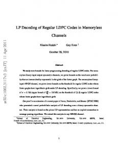
Then update the best factor pair of (g+1) (g+1) generation g + 1 to (αlbest , β lbest ), where µ ¶(g+1) L Eb . lbest = arg min l=1 No l Step 4 Stoping test and output: If Gmax is reached or the smallest threshold of generations stop decreasing, (g+1) (g+1) output (αlbest , β lbest ). Otherwise, go to Step 2. VII. S IMULATION RESULTS Figure 1 depicts the word error rate (WER) performance of the standard BP, 2-D normalized MS, conventional normalized MS and MS algorithms for decoding a (16200,7200) irregular LDPC code. The check and bit node distributions of this code are ρ(x) = 0.00006x2 + 0.14917x3 + 0.29851x4 + 0.44777x5 + 0.10449x6 and λ(x) = 0.00002 + 0.38803x + 0.31344x2 + 0.29851x7 , respectively. We observe that 2-D normalized MS provides a comparable performance as BP and interestingly has a lower error floor than that of BP in the high SNR region. We also observe that 2-D normalized MS outperforms conventional normalized MS and MS by about 0.3dB. For this (16200, 7200) irregular LDPC code, the thresholds computed by density evolution for standard BP, MS, conventional MS and 2-D normalized MS are 0.77dB, 0.93dB, 0.90dB and 0.85dB, respectively. The optimum normalization factor for 1-D normalized MS is α = 0.75 and the optimum normalization vectors of 2-D normalized MS are α = (1.00, 0.94, 0.92, 0.88, 0.86) and β = (1.00, 1.00, 0.91, 0.83). VIII. C ONCLUSION In this paper a 2-D normalized MS decoding has been presented to improve the performance of standard MS and normalized MS decoding. The proposed method requires considerably less complexity than that of BP while introducing small performance degradation compared with BP. It is interesting to note that in the high SNR region, 2-D normalized MS can have a lower error floor than that of BP. With respect to conventional normalized MS which can be viewed as a simplified version of 2-D normalized MS decoding, the presented method offers a better performance with negligible increased complexity. Simulation and density evolution show that 2-D normalized MS provides a good performance versus complexity tradeoff for decoding irregular LDPC codes. The method discussed in this paper can be extended to offset MS decoding of irregular LDPC codes [13]. ACKNOWLEDGEMENT The authors would like to express their gratitude to Jinghu Chen for many interesting discussions and constructive comments.
WER
and
−2
10
−3
10
−4
10
0.4
Standard BP 2−D Normalized Min−Sum 1−D Normalized Min−Sum Min−Sum 0.5
0.6
0.7
0.8
0.9 Nb/No(dB)
1
1.1
1.2
1.3
1.4
Fig. 1. WER of standard BP, 2-D normalized Min-Sum, conventional normalized Min-Sum and Min-Sum algorithms for decoding a (16200,7200) irregular LDPC code (Imax =200).
R EFERENCES [1] R. G. Gallager, Low-Density Parity-Check Codes. Cambridge, MA: M.I.T. Press, 1963. [2] J. Pearl, Probabilistic Reasoning in Intelligent Systems: Networks of Plausible Inference. San Mateo, CA: Morgan Kaufmann, 1988. [3] D. J. C. MacKay, “Good error-correcting codes based on very sparse matrices,” IEEE Trans. Inform. Theory, vol. 45, pp. 399-431, Mar. 1999. [4] T. J. Richardson and R. L. Urbanke, “The capacity of low-density paritycheck codes under message-passing decoding,” IEEE Trans. Inf Theory, vol.47, pp. 599-618, Feb. 2001. [5] T. J. Richardson, M. A. Shokrollahi, and R.L. Urbanke, “Design of capacity-approaching irregular low-density parity-check codes,” IEEE Trans. Inf Theory, vol.47, pp. 619-637, Feb. 2001. [6] J. Hagenauer, E. Offer and L. Papke, “Iterative decoding of block and convolutional codes,” IEEE Trans. on Inform., vol. 42, pp. 429-445, March 1996. [7] M. Fossorier, M. Mihaljevic and H. Imai, “Reduced complexity iterative decoding of low-density parity check codes based on belief propagation,” IEEE Trans. Commun., vol. 47, pp. 673-680, May 1999. [8] J. Chen and M. Fossorier, “Near optimum universal belief propagation based decoding of low-density parity-check codes,” IEEE Trans. Commun., vol. 50, pp. 406-414, Mar. 2002. [9] J. Chen, A. Dholakia, E. Eleftheriou, M. Fossorier and X.-Y. Hu, “Reduced-Complexity Decoding of LDPC Codes,” IEEE Trans. Commun., vol. 53, pp. 1288-1299, Aug. 2005. [10] X. Wei and A. N. Akansu, “Density evolution for low-density paritycheck codee under Max-Log-MAP decoding,”Electron. Lett., vol.37, pp. 1225-1226, Aug. 2001. [11] J. Chen and M. Fossorier, “Density evolution for two improved BP-sased decoding algorithms of LDPC codes,” IEEE Commun. Lett., vol.6, pp. 208-210, May 2002. [12] S. Y. Chung, “On the construction of some capacity-approaching coding schemes,” Ph.D. dissetation, MIT, Cambridge, MA, 2000. [13] J. Zhang, M. Fossorier, D. Gu, and J.Y. Zhang, “Two-Dimensional Correction for Min-Sum Decoding of Irregular LDPC Codes,” submitted to IEEE Commun. Lett.