IEEE TRANSACTIONS ON NEURAL SYSTEMS AND REHABILITATION ENGINEERING, VOL. 24, NO. 3, MARCH 2016
333
Improved Neural Signal Classification in a Rapid Serial Visual Presentation Task Using Active Learning Amar R. Marathe, Vernon J. Lawhern, Dongrui Wu, Senior Member, IEEE, David Slayback, and Brent J. Lance, Senior Member, IEEE
Abstract—The application space for brain–computer interface (BCI) technologies is rapidly expanding with improvements in technology. However, most real-time BCIs require extensive individualized calibration prior to use, and systems often have to be recalibrated to account for changes in the neural signals due to a variety of factors including changes in human state, the surrounding environment, and task conditions. Novel approaches to reduce calibration time or effort will dramatically improve the usability of BCI systems. Active Learning (AL) is an iterative semi-supervised learning technique for learning in situations in which data may be abundant, but labels for the data are difficult or expensive to obtain. In this paper, we apply AL to a simulated BCI system for target identification using data from a rapid serial visual presentation (RSVP) paradigm to minimize the amount of training samples needed to initially calibrate a neural classifier. Our results show AL can produce similar overall classification accuracy with significantly less labeled data (in some cases less than 20%) when compared to alternative calibration approaches. In fact, AL classification performance matches performance of 10-fold cross-validation (CV) in over 70% of subjects when training with less than 50% of the data. To our knowledge, this is the first work to demonstrate the use of AL for offline electroencephalography (EEG) calibration in a simulated BCI paradigm. While AL itself is not often amenable for use in real-time systems, this work opens the door to alternative AL-like systems that are more amenable for BCI applications and thus enables future efforts for developing highly adaptive BCI systems. Index Terms—Active learning, brain–computer interface, electroencephalography, rapid-serial visual presentation. Manuscript received February 23, 2015; revised May 26, 2015, July 10, 2015, and November 06, 2015; accepted November 07, 2015. Date of publication November 20, 2015; date of current version March 04, 2016. This project was supported by the Office of the Secretary of Defense Autonomy Research Pilot Initiative program MIPR DWAM31168, by the U.S. Army Research Laboratory, under Cooperative Agreement Number W911NF-10-2-0022 and through the Oak Ridge Institute for Science and Engineering under program MIPR 4LDATBP033. The views and the conclusions contained in this document are those of the authors and should not be interpreted as representing the official policies, either expressed or implied, of the U.S. Government. A. R. Marathe and V. J. Lawhern contributed equally to this work A. R. Marathe and B. J. Lance are with the Human Research and Engineering Directorate, U.S. Army Research Laboratory, Aberdeen Proving Ground, MD 21005 USA (e-mail:
[email protected]). V. J. Lawhern is with the Human Research and Engineering Directorate, U.S. Army Research Laboratory, Aberdeen Proving Ground, MD 21005 USA and with the Department of Computer Science, University of Texas at San Antonio, San Antonio, TX 78249 USA (e-mail:
[email protected]). D. Wu is with Data Nova, Clifton Park, NY 12065 USA. D. Slayback is with the Human Research and Engineering Directorate, U.S. Army Research Laboratory, Aberdeen Proving Ground, MD 21005 USA and with the Department of Computer Science, University of Pittsburgh, Pittsburgh, PA 15213 USA. Color versions of one or more of the figures in this paper are available online at http://ieeexplore.ieee.org. Digital Object Identifier 10.1109/TNSRE.2015.2502323
I. INTRODUCTION
T
HERE are vast amounts of human variability in neural activity, both within and across individuals. As a result, attempting to classify the neural activity found in modalities such as electroencephalography (EEG) requires extensive calibration prior to each use by an individual. This calibration requirement directly affects the development of brain–computer interface (BCI) technologies that rely on the classification of neural activity. Most real-time BCIs require a calibration period that can last from 5 to 20 min [1]. Furthermore, these systems tend to lack robustness over time due to decreased classifier performance caused by changes in human state, the surrounding environment, and task conditions that alter the relationship between brain activity and task. This need for extensive individualized calibration renders most BCI technologies inconvenient or impossible to use for many people. As a result, developing EEG classification methods that reduce this need for calibration will improve the usability of these systems. One promising approach for reducing individual calibration effort for EEG classification is through Active Learning (AL) [2]. AL is an iterative semi-supervised learning technique in which, at each iteration, an active learner (in this case, a machine learning algorithm such as a support vector machine (SVM)) identifies maximally informative data points, queries an oracle for ground-truth labels for those points, and then incorporates that labeled data into the training model for the next iteration. AL is an ideal approach for learning in situations in which data may be abundant, but labels for the data are difficult or expensive to obtain. Examples of this scenario include the following: speech recognition and annotation [3] where expert listeners manually identify spoken words in audio recordings; image and video classification [4] where experts manually categorize images and video based on image features; and document categorization and text classification [5] where experts determine categories of books and other written materials based on small paragraphs or chapters. As an example, human labeling of words in audio recordings have reported efforts of 8–10 times the length of audio recordings for full word annotation [6]. This represents an extremely expensive labeling task that may not be completely necessary to achieve optimal classification performance. In each of these scenarios, AL significantly reduces the amount of labeling effort needed to obtain comparable performance with full data set classification training.
1534-4320 © 2015 IEEE. Personal use is permitted, but republication/redistribution requires IEEE permission. See http://www.ieee.org/publications_standards/publications/rights/index.html for more information.
334
IEEE TRANSACTIONS ON NEURAL SYSTEMS AND REHABILITATION ENGINEERING, VOL. 24, NO. 3, MARCH 2016
However, while AL has enjoyed success in many research fields, it is not commonly used in EEG analysis. We believe the key reason for this is that AL requires an oracle to label the unlabeled data, and in many EEG classification tasks, the data may not be amenable to manual labeling. This is because manually labeling the EEG data is not a viable approach, as it is difficult or impossible to visually distinguish EEG data from two or more distinct conditions. However, there are situations in current BCI applications that could be amenable to AL given a slight change in the BCI paradigm being employed. Generally speaking, AL can be used by having the user be the oracle who provides the labels for uncertain data points in any paradigm in which either the BCI provides feedback to the user, or the user is directly queried about the output of the BCI. One example of this is P300 speller BCIs [7]. The P300 speller is a BCI system that provides the user a way to spell words based on the detection of the P300 waveform. Letters are commonly arranged in a 6 6 grid and flashed in differing patterns. The user then focuses on a particular letter so that the flashing of the letter induces a P300 waveform that is then detected by the BCI. Once the BCI system predicts the letter, it is shown to the user as system feedback. Previous research has shown that an error-related negativity (ERN) occurs when the predicted letter is not the letter that the user desires [7]. One possibility of applying AL to this situation is to ask the user if the letter is correct based on the presence of the ERN. This user feedback is then used to derive better decision boundaries for better initial classification of the P300 waveform and better detection of the ERN. Ideally, the user should not be queried too often as that disrupts the operation of the BCI; however, obtaining new labels when necessary can significantly improve the performance of the BCI. Our initial research has shown that AL can be applied to EEG signal classification. For example, in previous work [8], we used AL for classification of oddball images in single-trial visual-evoked potential (VEP) responses. We showed that AL, when combined with transfer learning, can significantly reduce the number of labeled user-specific data samples, and that in a few subjects, AL can hit a performance level similar to that of 5-fold cross-validation (CV) with labels for less than 20% of the data. We have also shown that combining transfer learning with active class selection, a variant of active learning, can be used to predict cognitive load in a virtual reality Stroop task with significantly reduced labeling effort [9]. However, both of these applications combined AL with transfer learning, and the effect of AL alone has not been thoroughly investigated. In this paper, we have identified a BCI application that is highly amenable to AL, which is the use of Rapid Serial Visual Presentation (RSVP) for image triage. We apply AL to a simulated BCI system for target identification using data from an RSVP paradigm to minimize the amount of training samples needed to initially calibrate the neural classifiers. In an RSVP paradigm, analysts are shown a sequence of images in rapid succession (e.g., 2–10 Hz) [10], [11] and asked to detect sparsely appearing images from a specific target class that appear in a series of non-target or distractor stimuli. When a target is detected in an image, a neural response commonly associated with the P300 event-related potential (ERP) is evoked and classified
by the BCI system [12]. Each image in an RSVP task is classified based on the neural response of the analyst. Images that are deemed most likely to contain targets are triaged for subsequent inspection by the analyst. RSVP-based BCI systems have enabled image analysts to detect targets in large aerial photographs faster and more accurately than traditional standard searches [13]–[20]. Traditionally, these systems have been calibrated by having an analyst identify known targets in an initial calibration RSVP stream, where all images are manually labeled as being from the target class or from the non-target class. Ideally, these labeled images should be a representative subset of the overall image set being analyzed. After this calibration procedure is finished, the neural classifiers are trained on the data by relating the neural responses collected to the labels provided by the analyst. The trained neural classifiers are then used in subsequent RSVP streams for target identification. Short calibration periods can reduce manual labeling effort (by reducing the overall number of trials to label), but this can also result in insufficient training data. Longer calibration periods provide more data for training; however, this results in increased manual labeling effort for the user. The main advantage of using AL in this paradigm is that the user is not required to label all the data but only the most informative data, which significantly reduces the labeling effort required to obtain a good initial calibration. Our AL implementation uses a Query-by-Committee (QBC) [21] approach with a heterogeneous ensemble of state-of-the-art neural classifiers serving as a committee that identifies the most informative data samples in need of a label. These most informative data samples are identified on the basis of an aggregate confidence score for each sample that is derived from the reliability of the prediction from each neural classifier [22], [23]. Our results show AL can maintain overall classification accuracy when trained with significantly less labeled data when compared to traditional calibration using 10-fold cross-validation and full label knowledge to train a classification model. Other studies have used semi-supervised learning techniques for classification of EEG signals that are similar to the work presented here. For example, Gu et al. [24] use an online updating least squares support vector machine (LS-SVM) classifier that uses its own predictions on the test data set to augment the training data set and to teach itself for better classification. This can be viewed as a form of pseudo-label training, which has been used successfully in training deep neural networks [25]. This approach was also used in Spüler et al. [26] for adaptive training of a classifier for detecting error-related potentials. Another approach uses a two-classifier co-training approach in which trials identified as most confident are incorporated into the training process [27], [28] using the classifier determined label. Selecting only the most confident trials for incorporation into the training set was also done in Qin et al. [29] in an online learning SVM. Our approach differs from these approaches in that trials that are least confident as determined by the committee of classifiers are incorporated into the training data set, with a label provided by an oracle. Finally, there is the possibility that a set of previously labeled images can be used for training, but this can result in poor classi-
MARATHE et al.: IMPROVED NEURAL SIGNAL CLASSIFICATION IN A RAPID SERIAL VISUAL PRESENTATION TASK USING ACTIVE LEARNING
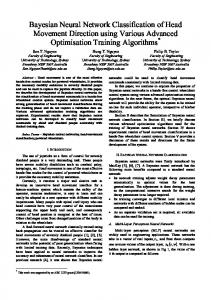
fier performance if the calibration images are non-representative of the overall task. For example, an inverse relationship between target frequency within an image and the strength of the overall ERP waveform has been shown in the literature [30]. Also, characteristics of the stimuli have been shown to impact the neural response and neural classification accuracy. For example, previous work has shown that target eccentricity and target size impact neural classification [31]. Other studies have shown that difficulty of target detection (which can be related to clutter, occlusion, and a variety of other factors) strongly impacts behavioral performance [32], which is strongly linked to neural classification performance [31]. Thus, using previously labeled data may not transfer well to new data if the characteristics of the labelled image set does not match the target data set. Instead, we propose using AL to obtain a representative, sufficiently sized training set with minimal manual labeling effort by intelligently labeling only the most informative data samples. While the results presented here focus on an offline analysis in which the training and testing sets are very similar in characteristics, a key aspect of demonstrating the viability of this approach is to embed it into an online BCI system with realtime feedback where AL enables the system to rapidly adapt to changes in the environment or in the user's performance. Admittedly, the number of BCI applications that are amenable to having a human oracle manually label data is limited; however, there are alternative AL-based methodologies that relax some of the strict rules of AL (cf. [33]–[35]), such as training in the absence of ground-truth label information for all data points, and using pseudo-labels learned from the ensemble as if they were the ground truth [25]. For example, an alternative oracle in this case could be a committee of computer vision algorithms trained to detect targets and non-targets from image features independent of neural features [22]. In any event, by demonstrating the viability of a strict AL implementation, we open the door to these alternatives, which are potentially applicable to a much broader space of BCI technologies. II. METHODS A. Participants 18 participants volunteered for the current study. Participants provided written informed consent, reported normal or corrected-to-normal vision, and reported no history of neurological problems. Data from 3 participants was discarded due to excessive artifacts and/or noise within the EEG data. The 15 remaining participants included nine male and 14 right-handed participants who ranged in age from 18–57 (mean age 39.5). The voluntary, fully informed consent of the persons used in this research was obtained as required by federal and Army regulations [36], [37]. The investigator adhered to Army policies for the protection of human subjects [37]. B. Stimuli and Procedure Fig. 1 shows an example RSVP stream used in the experiment, consisting of short video clips [38]. Video clips contained either people or vehicles in background scenes, or only background scenes. Participants were instructed to make a manual button press with their dominant hand when they detected a
335
Fig. 1. Visualization of the RSVP experiment used in this study. RSVP presentation rate was 2 Hz, with each presentation consisting of a 500 ms movie, shown as five images at 10 Hz rate. Each 500 ms block consisted of either a target or a non-target movie. Target classes included images containing people or vehicles, with non-targets shown as background images. Figure reproduced from Ries and Larkin [38] with permission.
person or vehicle (targets) and to abstain from responding when a background scene (distractor) was presented. Video clips consisted of five consecutive images, each 100 ms in duration; each video clip was presented for 500 ms. There was no interval between videos such that the first frame was presented immediately after the last frame of the prior video. Fifty percent of the video clips showed static scenes, meaning that all five images in the video clip were identical. The other 50% contained some type of motion (e.g., trees moving in the wind, car driving across the scene). If a target appeared in the video clip, it was present on each 100 ms image. The distracter to target ratio was 90/10. RSVP sequences were presented in 2 minute blocks after which time participants were given a short break. Additionally, to reduce the impact of ocular artifacts on the EEG data, a blink screen appeared every 10 seconds and remained on screen for 500 ms. Participants completed a total of 10 blocks. C. EEG Recording and Analysis Electrophysiological recordings were digitally sampled at 512 Hz from 64 scalp electrodes arranged in a 10-10 montage using a BioSemi Active Two system (Amsterdam, The Netherlands). External leads were placed on the outer canthi and below the orbital fossa of both eyes to record electrooculography (EOG). Continuous EEG data were referenced offline to the average of the left and right earlobes and digitally filtered 0.1–55 Hz. Extended Infomax Independent Components Analysis along with subsequent visual inspection of components was used to remove muscle and ocular artifacts from the EEG signal [39]. D. EEG Signal Classification Three different single-trial classification methods were used to determine the presence of an ERP related to the target. For each classifier, the EEG signals were first bandpass filtered (Butterworth filter of order 4) with cutoff frequencies at 1 and 10.66 Hz. The results of the competition in the 2010 IEEE Workshop on Machine Learning for Signal Processing [40] suggested that improved performance could be obtained by downsampling the EEG data to 32 Hz. In the current study, this downsampling was only beneficial for two of the three classifiers when using a 10-fold cross-validation and thus was only used for those
336
IEEE TRANSACTIONS ON NEURAL SYSTEMS AND REHABILITATION ENGINEERING, VOL. 24, NO. 3, MARCH 2016
two methods (XDawn+Bayesian Linear Discriminant Analysis and Common Spatial Patterns). The remaining classifier (Hierarchical Discriminant Component Analysis) used the original sampling rate of 512 Hz for classification. For each classifier, we then focused the subsequent analysis on 1 s of post-stimulus data. Details of each method are briefly described below. 1) Hierarchical Discriminant Component Analysis (HDCA): HDCA is a binary classification method based on an ensemble of logistic regression classifiers that transforms multi-channel EEG data collected over a temporal window relative to image onset into a single “interest score.” Ideally, the interest score is generated so that the range of scores for each class are distinct, thereby allowing for simple discrimination of the two classes. Generating interest scores from HDCA involves a two-stage classification. In the first stage, a set of 20 logistic regression discriminators are applied to 20 equally-sized, non-overlapping time windows that range from image onset up to 1 s post-image onset. Each of the 20 discriminators are trained independently. Each of these 20 discriminators serve to collapse the information contained in all 64 EEG channels collected over the course of the corresponding time window into a single value for discriminating between the neural signal evoked by the two image classes. In the second stage, a separate logistic regression discriminator is applied to the output of the 20 Stage 1 discriminators to create a single interest score that can efficiently discriminate the two image classes. The choice of 20 Stage 1 discriminators was largely based on previous studies [14], [41]; however, using 10 Stage 1 discriminators (100 ms time windows) has also been done [42] and produced no significant differences in the classification performance reported here. 2) Common Spatial Patterns (CSP): The second classification method used here combined CSP spatial filtering with a Bayesian linear discriminant analysis (BLDA) classifier. CSP creates linear combinations of signals that maximize the difference in signal variance between two known conditions [43], [44]. In our implementation, eight spatial filters were used for the classifier input. The input vector was obtained by concatenation of the eight spatially filtered EEG signals, and the BLDA classifier was used to discriminate targets from non-targets [45], [46]. 3) XDawn+Bayesian Linear Discriminant Analysis (XDBLDA): The third classification method employed here used a combination of the XDawn spatial filtering technique coupled with a BLDA classifier. Collectively, this technique will be referred to as XDBLDA and a full description can be found in Rivet et al. [47] and Cecotti et al. [48], [49]. XDawn spatial filtering results in a set of spatial filters that are rank ordered such that the highest rank filters maximize the signal-to-signal-plus-noise ratio in the EEG signals. Just as with CSP, our implementation used the top eight spatial filters for classifier input, and the input vector was obtained by concatenating the eight spatially filtered EEG signals. The BLDA classifier was then used to discriminate targets from non-targets. 4) Confidence: Confidence measures were derived for each neural classifier to identify the reliability of the classification made for each trial. Similar approaches have been used in previous RSVP studies as a means to sort the images by likelihood
of containing a target to improve the speed of target detection [41], [42], [50], [51]. Here, we defined the confidence measure as the distance of a given classifier score from the discriminating boundary. The utility of this approach has been previously presented [22], [23], and a more in-depth analysis is being done in a separate study. Confidence was calculated as follows: (1) Here, Score was the score produced on a single trial, max(Score) and min(Score) were the maximum and minimum observed values of Score across all trials in the training set, respectively, and threshold was the discriminating boundary, which was defined as the value that maximized the difference between the true positive rate and false positive rate in the training set. 5) Merging Classifier Output: For each neural classifier, a prediction of target/non-target (coded as ) and a confidence score were obtained. We merged the two outputs to create new covariate variables for each classifier (one each for HDCA, CSP, and XDBLDA) by multiplying the binary prediction variable with the confidence score for each trial. This produced a continuous measure where larger positive values indicated higher confidence in target, while larger negative values denoted higher confidence in non-target. Values near 0 (either positive or negative) denoted a lower degree of confidence. We then fit an ensemble classifier using logistic regression that predicted individual trials as being from the target class or non-target class using the outputs of the three neural classifiers (HDCA, CSP, and XDBLDA) as covariates. We used step-wise regression to select a statistically significant model from among the three covariates using the model deviance as the criterion. The difference in deviances between two models is a statistical measure of the quality of a model fit and follows an approximate distribution with degrees of freedom, with being the difference in the number of parameters in the model [52]. Note that for a step-wise search. We will use the terminology “joint decision” to refer to this logistic regression fusion of the outputs of HDCA, CSP, and XDBLDA for the remainder of the manuscript. 6) Cross-Validation (CV): For the purpose of statistical testing, for each classifier we performed 10-fold CV in which the data is divided into 10 non-overlapping blocks and classifiers were trained on all but one block and tested against the remaining block. This was done 10 times so that each block was used as the testing set. The overall CV accuracy is then reported as the average of the 10 testing set accuracies. E. Active Learning As a means to minimize calibration effort, AL selects the most informative samples to label so that a given learning performance can be achieved with less labeling effort. A hypothetical illustration of AL is shown in Fig. 2. Suppose there are two classes (stars and triangles), which are separated by some true underlying decision boundary [shown as a dashed purple circle in Fig. 2(a)] and an estimated decision boundary [shown in dashed black in Fig. 2(b)] obtained from a
MARATHE et al.: IMPROVED NEURAL SIGNAL CLASSIFICATION IN A RAPID SERIAL VISUAL PRESENTATION TASK USING ACTIVE LEARNING
337
Fig. 2. Illustration of AL. (A) True underlying distribution, which is assumed unknown, of a binary decision space, with red triangles and purple stars denoting two distinct classes. The dashed purple line denotes the underlying decision boundary. (B) An estimated decision boundary (black dashed) given three labeled samples from each class. Grey circles denote unlabeled samples. (C) An estimated decision boundary given two additional labeled samples (black arrows) as determined by AL. (D) An estimated decision boundary given two additional labeled samples that have been selected at random. This represents the SizeBaseline (SB) measure described in Table I. Note that these newly labeled samples provide no additional information, so the original decision boundary is sufficient. (E) An estimated decision boundary given two additional labeled samples drawn from the same class as the two samples learned from AL in (C). This measure represents the potential improvement in the estimated decision boundary when knowledge of the class distribution is known (see the ClassBaseline [CB] measure in Table I). Note that the decision boundaries in (C) and (E) more accurately resemble the true decision boundary, with (C) having the best representation.
classifier learning on six labeled samples (shown as red triangles and purple stars). This decision boundary can be estimated by any classification routine (for example, logistic regression or SVMs). The problem domain of AL is that we are given only a few labeled samples from each class to learn this initial decision boundary. Given this limitation, our task is to select a few more samples, obtain the labels for those few samples, and incorporate their information into the classification efficiently. One possible strategy is to select points at random (Fig. 2(d), arrows); however, there exists a possibility that these points will not provide any significant information. AL instead uses a heuristic to estimate informative points for labeling and re-estimates the decision boundary using this new information (Fig. 2(c), arrows). Several strategies have been proposed to select these samples. Examples include QBC [21] and uncertainty sampling [53], [54]. QBC selects points by forming a committee of classifiers (usually homogeneous classifiers provided by a k-fold CV) and finding points where classifiers disagree on class labels, whereas uncertainty sampling uses a heuristic to estimate uncertain points and samples data points with the lowest certainty. One example of such a heuristic is a distance-to-decision boundary metric (used in Fig. 2). In this work, we used a combination of QBC and uncertainty sampling by using HDCA, CSP, and XDBLDA as our committee of classifiers and an unweighted linear summation of each classifier's confidence score (see Section II-D-4) as the uncertainty metric. Pseudocode for our AL implementation is shown in Fig. 3. A flowchart of the AL process is shown in Fig. 4. We assumed all the data was initially unlabeled (shown in orange in Fig. 4). The data was then partitioned into three sets: training
Fig. 3. Pseudocode for AL algorithm. Note that the joint decision classifiers are trained using the classifiers from Step 1; however, the output of the joint decision classifier is not considered when performing the AL-based update in Steps 2 and 3.
, testing , and validation . The training and validation sets were then sent to the oracle for labeling. The validation
338
IEEE TRANSACTIONS ON NEURAL SYSTEMS AND REHABILITATION ENGINEERING, VOL. 24, NO. 3, MARCH 2016
Fig. 4. Diagram for AL. Numbers in parentheses correspond to the steps in the pseudocode shown in Fig. 3. The initial data set, assumed unlabeled (orange), is partitioned into three separate data sets: Training (X), Testing (Y), and Validation (V). The Training and Validation sets are then manually labeled by the user (green). Step (1) consists of training all neural classifiers on X and evaluating performance on Y and V. Classifier-labeled instances are shown in blue. Step (2) identifies the K trials with lowest confidence as labeled by the classifier (red) and removes them from Y. Step (3) queries the labels for the lowest confidence trials and then merges these labels with X. These steps are repeated until either a desired level of accuracy is obtained in V or a fixed number of iterations have been completed. The latter approach has been used in this study.
set was a random selection without replacement of 10% of the trials such that the ratio of target to non-target trials is reflective of the ratio in the overall data set. From the remaining trials, the training set was chosen by randomly selecting, without replacement, 15 target and 15 non-target trials. This initial balancing of the training set helps to produce accurate decision boundaries. All remaining trials were then placed into the test set . Step 1, shown as (1) in Fig. 4, starts with training all neural classifiers using and evaluating the performance on using the area under the receiver operating characteristic (ROC) curve performance metric. The ROC curve is a plot of the true positive rate against the false positive rate, across a range of possible discriminating threshold values. Taking the area under this curve (the AUC) produced a measure of classifier efficacy. In Step 2, the trained model was evaluated on the testing set and the aggregate confidence was calculated for each trial. The trials with the least overall confidence were then removed from (see Step 2 in Fig. 4). In Step 3, these trials were sent to the oracle for labeling (see Step 3 in Fig. 4). In our simulations, the oracle was assumed to be the user, given unlimited time, who labels each image as being from either the target or non-target class. Once the low confidence trials were labeled, they were merged into the training set , whereby the process started anew at Step 1. This process continued for a pre-determined number of iterations. In this work, we set the number of iterations to be 100, and we set for our analysis. F. Statistical Analysis We conducted a series of simulations to validate the improved performance of the AL classification models against three baselines. In the first baseline, we compared the AL performance at each iteration to the 10-fold CV classification (Section II-D-6). The 10-fold CV classification provided an estimate of overall classification accuracy given full data annotation, and as such,
TABLE I SUMMARY OF DATA SELECTION METHODS
For each of the methods described here, the data selection criteria described in this table replaces the data selection portion of Step 3 in the pseudocode above. The 10-fold CV baseline condition is not shown here as there is no iterative ‘Data Selection Criteria’ for this method.
was an effective baseline to compare the overall performance of the AL-derived classifiers. Two additional baselines were required to validate the effectiveness of the AL process for iteratively improving classifier performance. The first of these additional baselines, called SizeBaseline (SB), was calculated by selecting points at random instead of selecting based on aggregate confidence [Table I, Fig. 2(d)]. This baseline controlled for the effect of improved performance based purely on increased sample size and offered the same performance as a set of standard block organized CV tests in which a given fraction of the data was used for training. The final baseline, called ClassBaseline (CB), selected points at random, but followed the same class distribution that was selected using AL [Table I, Fig. 2(e)]. For example, if in AL the and trials were selected from Classes 1 and 2, respectively, then CB randomly selected trials from Class 1 and trials from Class 2 from all available trials in . Whereas SB controlled for the effect of sample size, CB controlled for whether the aggregate confidence accurately identified useful trials and statistically controlled for
MARATHE et al.: IMPROVED NEURAL SIGNAL CLASSIFICATION IN A RAPID SERIAL VISUAL PRESENTATION TASK USING ACTIVE LEARNING
the effect that class distribution may have on the overall performance. Note that the AL analysis was performed prior to the CB analysis since the class distribution was only known after the AL analysis was performed. Furthermore, the CB analysis assumed that all labels in are known a priori since we were randomly sampling trials of specific sizes from each class. Therefore, the CB analysis was used only as a statistical measure of improved performance and does not represent a viable alternative to AL. Each of the three different methods (AL, SB, CB) was simulated 100 times, with a total of iterations per simulation. The 30 initial trials plus the additional 1000 trials added over the course of the 100 iterations (10 trials per iteration) resulted in a final training set of 1030 trials. For the purpose of presenting the results, the number of trials in the training set at each iteration was converted to a percentage of the total number of trials available. To assess the overall performance among the three methods (AL, CB, SB), we defined a novel measure called the AreaUnder-Performance-Curve (AUPC) as the area under the curve of the AUC values plotted for each iteration normalized so that the range of One AUPC value is obtained for each simulated run, so AL, CB, and SB will each have 100 AUPC values for each subject. Our statistical testing procedure was performed in multiple stages. In the first stage, we checked for an overall difference in AUPC for each subject by performing a non-parametric analysis of variance (ANOVA) (Kruskal-Wallis), using AL, CB, and SB as the three factors. If this overall test was significant, we then performed non-parametric ANOVAs on the AUC values at each iteration to determine which iteration produced significant deviations. If this test was significant at iteration , we performed further post-hoc pairwise analyses (TukeyKramer) to determine which method (AL, CB, SB) had significantly different AUC values. False-Discovery Rate (FDR) analyses were used to control for the effect of multiple comparisons [55], [56].
339
Fig. 5. Comparison of AUPC across all subjects with AL, CB, and SB for the joint decision classification. Error bars denote one standard deviation across the 100 repetitions for the individual subjects. For the “Avg,” error bars denote one standard deviation across the subject means. Note: 10-fold CV baseline is not included here because the AUPC measure requires an iteratively trained classifier to measure performance.
III. RESULTS AL produces more accurate classifiers with less manually labeled data than both CB and SB (Fig. 5). For each of the 15 subjects, the average AUPC for the joint decision classifier trained using AL is greater than comparable classifiers trained with CB, which is in turn greater than classifiers trained with SB. This result is intuitive given that CB gives some additional information that helps in estimating a better decision boundary [Fig. 2(e)]. The difference across the three conditions is statistically significant (individual Kruskal-Wallis tests per subject with FDR adjustment, ). Subsequent post-hoc comparisons using Tukey-Kramer (see Section II-F) show that AL has larger values than both CB and SB for nearly all subjects. In addition to outperforming CB and SB, for a majority of subjects, AL performance was similar to the performance of 10-fold CV when training with substantially less training data (Fig. 6). Fig. 6(a) compares the AUC values for AL, CB, and SB when using 5%, 25%, and 50% of the data for training the joint decision classifier (see Section II-D-5) with the performance of the 10-fold cross-validated joint decision classifiers trained on 90% of the data. When 25% of the data is used for training, the
Fig. 6. (A) AUC for AL, CB, and SB using 5%, 25%, and 50% of the data for training compared to a 10-fold cross-validated classifier that uses 90% of the trials for training. Error bars represent standard deviation. (B) Plot of the percentage of subjects whose average AL performance exceeded average 10-fold CV performance by size of training data set in percent for the three different selection methods. All performance values were measured based on the joint decision classification.
340
IEEE TRANSACTIONS ON NEURAL SYSTEMS AND REHABILITATION ENGINEERING, VOL. 24, NO. 3, MARCH 2016
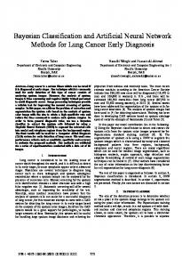
Fig. 7. Classification performance for Subject S08. (A)–(D) AUC values for the three neural classifiers (HDCA, XDBLDA, CSP) and a joint decision classifier, respectively, as a function of the percent of trials used for training. The three curves within each subfigure denote AL (blue), CB (green), and SB (red) performances, and the dashed horizontal line denotes the 10-fold CV performance for that specific classification method, which uses 90% of the data for training. Error bars denote a 95% bootstrap confidence interval. (E) Percentage of AL bootstrap models containing significant parameters based on the percent of data included in the training data set. Nearly all bootstrap models contain all three neural classifiers as statistically significant variables with the exception of CSP in the earlier iterations and XDBLDA in the later iterations.
mean AL AUC performance for 3 out of 15 subjects ( 35%) is greater than the mean AUC of 10-fold CV. This trend continues until the data in the training set is about 50%, where over 70% of subjects had mean AUC values greater than the mean AUC of 10-fold CV. In contrast, with the CB approach, only 35% of subjects had mean AUC performance greater than 10-fold CV at 50% training data [Fig. 6(b)]. The SB approach does not exhibit greater performance until about 50% training data size. As expected, individual performance across the population of subjects varies considerably. For 10 of the 15 subjects, the joint decision classifier using AL outperforms each of the individual committee members using AL. For Subject S08, highlighted in Fig. 7, the performance of the AL joint decision classifier is better than any individual AL classifier. In contrast, the joint decision does not perform better than any individual classifier with the CB (green) and SB (red) measures; in fact, the SB joint decision appears to perform worse than the SB HDCA measure at nearly all labeled data set sizes. This suggests that
AL is providing unique information at the joint decision classification level that is not present in the joint decision classifiers trained with CB and SB. For the other five subjects, the joint decision classifier using AL matched the top performing individual classifier using AL (Figures S1 and S2), whereas with SB and CB, the joint decision sometimes appears to perform worse than the individual classifiers. Across the entire group of subjects, the combination of using the joint decision classifier with AL appears to provide the overall best performance. An important consideration is whether each classifier is required for the joint decision AL classifiers to be successful. In general, the utility of each classifier varies across the population. For some subjects, all three classifiers are significant for most of the iterations (see Fig. 7). For this particular subject (S08), HDCA is always significant in all iterations across all bootstrap runs [Fig. 7(e)] ( test, , see Section II-D-5) except for the first few iterations. CSP and XDBLDA are significant in over 80% of bootstrap iterations at nearly all training set sizes except for CSP below 10% training set size and XDBLDA greater than 40% training set size. At around the 15%–25% range, all three classifiers are almost always significant. This interval coincides with the best observed tradeoff between classifier accuracy (accuracy matching that of 10-fold CV) and labeling effort [see Fig. 7(d)]. For some subjects, only two of the three classifiers are always significant (Figure S1). Other subjects (Figure S2) show that the significant classifiers vary across iterations. These differences across the population of subjects as to which classifiers will be important indicate that including all three classifiers would maximize performance of the joint decision AL classifier. IV. DISCUSSION This paper focuses primarily on using Active Learning to efficiently label a previously unlabeled image dataset using a reduced number of manual labels. We show that, in most cases, comparable classification performance to that of 10-fold crossvalidation can be achieved with significantly fewer labeled samples. This suggests that Active Learning can be used to reduce the calibration effort of the user by minimizing the number of labels the user must provide. The reduced labeling effort comes at a cost of computational time. The iterative nature of AL requires that each classifier be trained several times during a single calibration session. In many cases, the ability to trade increased labeling effort for an image analyst for increased processing load for a computer may be reason enough to warrant moving towards an AL based approach. However, even in cases where the amount of analyst time is in abundance, the AL approach can be more efficient given a sufficiently large data set (e.g., 1000 or more images). Given that traditional BCIs are often expected to function without overt responses, an important issue is whether the AL results presented here rely on the motor responses. Previous work has shown that HDCA can effectively classify neural responses in the absence of motor responses [41]. While similar studies involving XDBLDA and CSP have not been done, the aforementioned study implies that the underlying neural signal needed to classify target images is still present in trials without
MARATHE et al.: IMPROVED NEURAL SIGNAL CLASSIFICATION IN A RAPID SERIAL VISUAL PRESENTATION TASK USING ACTIVE LEARNING
an overt motor response, and thus XDBLDA and CSP should be able to function on this type of data as well. There does seem to be a small drop in performance between motor response data and non-motor response data (0.92 to 0.91 AUC in Gerson, et al. [41]). Based on this data, one would expect that the overall classification results may decline by a small amount in the absence of a motor response. Importantly, however, any decline in classifier accuracy is likely to similarly affect AL, CB, and SB (and any cross-validated classification) such that the main findings of this study would be unaltered. A. Understanding the Basis of Improved Performance The data presented here demonstrates that a majority of subjects exhibited an improvement in the mean classification AUC when using AL versus 10-fold CV. The underlying basis for this improvement is currently unclear. It is commonly understood in the machine learning literature that aggregating the outputs of multiple learning algorithms tends to provide more robust performance by exploiting independent information across multiple information sources. Our results have mainly corroborated this point. We have shown that using AL together with ensemble learning can significantly improve overall classification performance over AL with each member of the ensemble trained individually. However, it is currently unclear if the improved performance can also be tied to specific underlying neural features that are captured by AL but not captured by training using traditional approaches. In an attempt to answer this question, we have performed some initial exploratory analyses looking at the properties of the ERPs, the stimuli, and the behavioral response. However, none of these exploratory analyses clearly reveals the underlying neural basis, implying that there may be several factors underlying the improved performance of the AL algorithm, or that the improvement is non-neural in nature. 1) ERP Characteristics: One possibility for the improved performance of classifiers trained with AL is in the characteristics of the ERPs of the informative trials selected by the AL algorithm. We hypothesize that these will contain a smaller difference wave between the two classes, and that learning on these trials produces a more robust decision boundary. To test this, we compared the difference wave between target and non-target ERPs from the training set of the AL iteration that produced the best overall accuracy to the difference wave between target and non-target ERPs calculated using the full data for each subject. Using the area under the difference wave as a measure of similarity, we fit a linear regression, using the AUC value at the optimal AL iteration as the response variable and the area under the ERP difference waveforms as the predictor. However, this linear regression was significant in only 2 of the 15 subjects in the study, indicating that this was not the major factor in explaining the improved performance seen with AL. Previous research has also shown that an extended time-ontask may also cause decrements in the ERP waveform [57]. Thus, it is possible that AL was able to preferentially select trials near the end of a session, when time-on-task effects would have diminished the ERP amplitude, to include in the training set. We tested this by first dividing the total length of the experiment into 10 non-overlapping time windows and finding the number of trials in each of these windows at the AL iteration that produced the best overall AUC. We then performed a
341
test to determine if the distribution of trials in each bin was different than the expected number of trials in each bin (1/10th the total number of trials). This test was not significant in all subjects (FDR-corrected, ), which again indicates that this test was not the major factor in explaining the improved performance with AL. 2) Stimulus Type: Target and non-target images were presented either statically or in short movie clips, occurring with equal proportion [38]. Prior research suggests that moving images elicit more robust neural responses than static images. Since AL attempts to identify the trials that are more difficult to classify (e.g., the most informative trials), then it is possible that AL was preferentially selecting the static trials to add to the training set. To test this, we calculated the proportion of trials that fell into the static class within the AL-identified training set in each AL simulation, and we performed a non-parametric sign-rank test to test if the distribution of proportions had a median of 0.5, versus the alternative that the proportion was greater than 0.5. If this test is significant, this suggests that AL is identifying more trials belonging the static image class. While we did observe statistically significant differences in most subjects , across all subjects this difference was not significantly correlated with AL performance. This was determined by fitting a linear regression, with the mean AUC across all bootstrap iterations as the response and the mean proportion of moving images across all bootstrap iterations as the predictor. These values were calculated for each subject, resulting in 15 data point pairs. A t-test for a significant slope parameter ( , , where is the slope parameter) was not significant . We also tested this hypothesis non-parametrically using a bootstrap permutation . These procedure, which showed similar results results indicate that the stimulus type (moving versus static) was not the major factor responsible for the improvement seen in AL. 3) Behavioral Variability: An additional hypothesis was that subjects who demonstrated higher degrees of response time variability would show greater improvement in classification performance using AL. The reasoning behind this hypothesis stems from the fact that previous work has shown that increased levels of response time variability decreases classification accuracy [58], [59]. In both of these studies, removing the variability, either by removing the extremely long and extremely short latency trials, or by aligning trials to the behavioral response, dramatically improved classification accuracy. For subjects with a high degree of variability, AL may be improving performance by identifying a subset of trials with less variability and thereby approximating the effect of ignoring the extremely long and short latency trials [59]. To test this, we compared the reaction time of the AL-selected trials to the reaction time in the remaining trials. In a majority of subjects, the reaction time of the AL-selected trials showed very little difference from the reaction time of the remaining trials (t-test between AL-selected trials and remaining trials, for 11 of 15 subjects). In a small number of subjects, AL preferentially chose slightly faster trials, while in other subjects, AL preferentially chose slightly slower trials. Next, we compared the improvement in classification achieved through AL against the improvement in classification
342
IEEE TRANSACTIONS ON NEURAL SYSTEMS AND REHABILITATION ENGINEERING, VOL. 24, NO. 3, MARCH 2016
when response time variability is removed by aligning the trials to the timing of the behavioral response. AL was unable to match the performance increase achieved by removing response time variability; however, the joint decision classifiers produced through AL do match the performance of other classification approaches designed to overcome the temporal variability of neural response [58]. Our interpretation is that in some participants, the improvement seen through AL is predominantly driven by accounting for response time variability, while in other participants AL improvement is predominantly driven by other factors. Overall, these exploratory analyses cannot fully explain the neural basis for the improvement in classification using AL; however, they do indicate that the ERP characteristics, stimulus class type, and behavioral variability each may play some role in enabling AL to improve classification performance. Further analysis is required to appropriately characterize the relationship between these factors and the observed performance improvements. V. CONCLUSION This paper shows that AL can be used to more efficiently, and in some cases more accurately, calibrate a simulated BCI. However, the results presented here illustrate an interesting phenomenon. A general rule of thumb in the machine learning field is that classifiers built on larger training sets perform as well as or better than classifiers built on smaller training sets. Our results, however, are contrary to this in that we are able to show improved classification with smaller training set sizes with many of our subjects by intelligently choosing which data to include in the training set. For online learning, this would mean that rather than retraining classifiers using all of the new data, a previously trained classifier may only need a small subset of new data to recalibrate the existing classifier based on the new signal dynamics observed. This type of approach has produced good results in other fields [49], [50], and our results indicate that it may also be useful for BCI applications. REFERENCES [1] J. van Erp, F. Lotte, and M. Tangermann, “Brain-computer interfaces: Beyond medical applications,” Computer, vol. 45, no. 4, pp. 26–34, Apr. 2012. [2] B. Settles, Active learning literature survey Univ. Wisconsin, Madison, Comput. Sci. Tech. Rep. 1648, 2010. [3] X. Zhu, Semi-supervised learning literature survey 2005. [4] A. J. Joshi, F. Porikli, and N. P. Papanikolopoulos, “Scalable active learning for multiclass image classification,” IEEE Trans. Pattern Anal. Mach. Intell., vol. 34, no. 11, pp. 2259–2273, Nov. 2012. [5] S. Tong and D. Koller, “Support vector machine active learning with applications to text classification,” J. Mach. Learn. Res., vol. 2, pp. 45–66, 2002. [6] X. Zhu, “Semi-supervised learning with graphs,” Ph.D. dissertation, Dept. Psychology, Carnegie Mellon Univ., Pittsburgh, PA, 2005. [7] M. Perrin, E. Maby, S. Daligault, O. Bertrand, and J. Mattout, “Objective and subjective evaluation of online error correction during P300based spelling,” Adv. Hum.-Comp. Int., vol. 2012, p. 4:4-4:4, Jan. 2012. [8] D. Wu, B. J. Lance, and V. Lawhern, “Active transfer learning for reducing calibration data in single-trial classification of visually-evoked potentials,” in Proc. IEEE Int. Conf. Syst., Man, Cybern., San Diego, CA, 2014, pp. 2801–2807. [9] D. Wu, B. J. Lance, and T. D. Parsons, “Collaborative filtering for brain-computer interaction using transfer learning and active class selection,” PLoS ONE, vol. 8, no. 2, p. e56624, Feb. 2013.
[10] M. M. Chun and M. C. Potter, “A two-stage model for multiple target detection in rapid serial visual presentation,” J. Exp. Psychol., Human Perception Performance, vol. 21, no. 1, pp. 109–127, 1995. [11] M. C. Potter, “Short-term conceptual memory for pictures.,” J. Exp. Psychol., Human Learn. Memory, vol. 2, no. 5, p. 509, 1976. [12] E. A. Pohlmeyer et al., “Closing the loop in cortically-coupled computer vision: A brain–computer interface for searching image databases,” J. Neural Eng., vol. 8, no. 3, p. 036025, Jun. 2011. [13] P. Sajda et al., “In a blink of an eye and a switch of a transistor: Cortically coupled computer vision,” Proc. IEEE, vol. 98, no. 3, pp. 462–478, 2010. [14] L. C. Parra et al., “Spatiotemporal linear decoding of brain state,” IEEE Signal Process. Mag., vol. 25, no. 1, pp. 107–115, 2008. [15] E. A. Pohlmeyer et al., “Closing the loop in cortically-coupled computer vision: A brain–Computer interface for searching image databases,” J. Neural Eng., vol. 8, no. 3, p. 036025, 2011. [16] A. Kapoor, P. Shenoy, and D. Tan, “Combining brain computer interfaces with vision for object categorization,” in Proc. IEEE Conf. Comput. Vis. Pattern Recognit., 2008, pp. 1–8. [17] N. Bigdely-Shamlo, A. Vankov, R. R. Ramirez, and S. Makeig, “Brain activity-based image classification from rapid serial visual presentation,” IEEE Trans. Neural Syst. Rehabil. Eng., vol. 16, no. 5, pp. 432–441, Oct. 2008. [18] P. Poolman, R. M. Frank, P. Luu, S. M. Pederson, and D. M. Tucker, “A single-trial analytic framework for EEG analysis and its application to target detection and classification,” NeuroImage, vol. 42, no. 2, pp. 787–798, Aug. 2008. [19] J. Touryan, A. J. Ries, P. Weber, and L. Gibson, “Integration of automated neural processing into an army-relevant multitasking simulation environment,” in Foundations of Augmented Cognition, D. D. Schmorrow and C. M. Fidopiastis, Eds. Berlin, Germany: Springer, 2013, pp. 774–782. [20] M. Birisan and P. A. Beling, “A multi-instance learning approach to filtering images for presentation to analysts,” Environ. Syst. Decis., vol. 34, no. 3, pp. 406–416, Aug. 2014. [21] A. Krogh and J. Vedelsby et al., “Neural network ensembles, cross validation, active learning,” Adv. Neural Inf. Process. Syst., pp. 231–238, 1995. [22] A. R. Marathe, B. J. Lance, K. McDowell, W. D. Nothwang, and J. S. Metcalfe, “Confidence metrics improve human-autonomy integration,” in Proc. ACM/IEEE Int. Conf. Human-Robot Interact., New York, NY, USA, 2014, pp. 240–241. [23] A. R. Marathe et al., “The effect of target and non-target similarity on neural classification performance: A boost from confidence,” Front. Neurosci., vol. 9, p. 270, 2015. [24] Z. Gu, Z. Yu, Z. Shen, and Y. Li, “An online semi-supervised brain–computer interface,” IEEE Trans. Biomed. Eng., vol. 60, no. 9, pp. 2614–2623, Sep. 2013. [25] D.-H. Lee, “Pseudo-label: The simple and efficient semi-supervised learning method for deep neural networks,” presented at the ICML 2013 Workshop : Challenges in Representation Learning (WREPL), Atlanta, GA, 2013. [26] M. Spüler, W. Rosenstiel, and M. Bogdan, “Online adaptation of a c-VEP Brain-computer Interface (BCI) based on error-related potentials and unsupervised learning,” PLoS ONE, vol. 7, no. 12, p. e51077, 2012. [27] R. C. Panicker, S. Puthusserypady, and Y. Sun, “Adaptation in P300 brain-computer interfaces: A two-classifier cotraining approach,” IEEE Trans Biomed. Eng., vol. 57, no. 12, pp. 2927–2935, Dec. 2010. [28] S. Lu, C. Guan, and H. Zhang, “Unsupervised brain computer interface based on intersubject information and online adaptation,” IEEE Trans. Neural Syst. Rehabil. Eng., vol. 17, no. 2, pp. 135–145, Apr. 2009. [29] J. Qin, Y. Li, and W. Sun, “A semisupervised support vector machines algorithm for BCI systems,” Comput. Intell. Neurosci., vol. 2007, 2007. [30] H. Cecotti et al., “Impact of target probability on single-trial EEG target detection in a difficult rapid serial visual presentation task,” in Proc. Annu. Int. Conf. IEEE Eng. Med. Biol. Soc., 2011, pp. 6381–6384. [31] J. C. Dias and L. C. Parra, “No EEG evidence for subconscious detection during Rapid Serial Visual Presentation,” in Proc. IEEE Signal Process. Med. Biol. Symp., 2011, pp. 1–4. [32] S. Mathan, K. Hild, Y. Huang, and M. Pavel, “Characterizing the performance limits of high speed image triage using Bayesian search theory,” in Foundat. Augment. Cognit. Direct. Future Adaptive Syst., 2011, pp. 95–103. [33] P. Donmez and J. G. Carbonell, “Proactive learning: Cost-sensitive active learning with multiple imperfect oracles,” in Proc. 17th ACM Conf. INFORMATION Know. Management, 2008, pp. 619–628.
MARATHE et al.: IMPROVED NEURAL SIGNAL CLASSIFICATION IN A RAPID SERIAL VISUAL PRESENTATION TASK USING ACTIVE LEARNING
[34] Y. Yan et al., “Modeling annotator expertise: Learning when everybody knows a bit of something,” in Proc. Int. Conf. Artif. Intell. Stat., 2010, pp. 932–939. [35] B. Zhong et al., “Visual tracking via weakly supervised learning from multiple imperfect oracles,” Pattern Recognit., vol. 47, no. 3, pp. 1395–1410, 2014. [36] Code of Federal Regulations, Protection of Human Subjects. 32 CFR 219. Washington, DC: Govt. Print. Office, U.S. Dept. Defense Office Secretary Defense, 1999. [37] Use of Volunteers as Subjects of Research. AR 70-25. Washington, DC: Government Printing Office, 1990, U.S. Department of the Army. [38] A. J. Ries and G. B. Larkin, Stimulus and response-locked P3 activity in a dynamic rapid serial visual presentation (RSVP) task DTIC Document, 2013. [39] T. P. Jung et al., “Removing electroencephalographic artifacts by blind source separation,” Psychophysiology, vol. 37, no. 2, pp. 163–178, Mar. 2000. [40] J. M. Leiva and S. M. Martens, “MLSP competition, 2010: Description of first place method,” in Proc. IEEE Int. Workshop Mach. Learn. Signal Process., 2010, pp. 112–113. [41] A. D. Gerson, L. C. Parra, and P. Sajda, “Cortically coupled computer vision for rapid image search,” IEEE Trans. Neural Syst. Rehabil. Eng., vol. 14, no. 2, pp. 174–179, Jun. 2006. [42] P. Sajda et al., “In a blink of an eye and a switch of a transistor: Cortically coupled computer vision,” Proc. IEEE, vol. 98, no. 3, pp. 462–478, Mar. 2010. [43] B. Blankertz, R. Tomioka, S. Lemm, M. Kawanabe, and K.-R. Muller, “Optimizing spatial filters for robust EEG single-trial analysis,” IEEE Signal Process. Mag. , vol. 25, no. 1, pp. 41–56, Dec. 2008. [44] Y. Wang, P. Berg, and M. Scherg, “Common spatial subspace decomposition applied to analysis of brain responses under multiple task conditions: A simulation study,” Clin. Neurophysiol., vol. 110, no. 4, pp. 604–614, 1999. [45] U. Hoffmann, J.-M. Vesin, T. Ebrahimi, and K. Diserens, “An efficient P300-based brain—Computer interface for disabled subjects,” J. Neurosci. Methods, vol. 167, no. 1, pp. 115–125, 2008. [46] D. J. MacKay, “Bayesian interpolation,” Neural Comput., vol. 4, no. 3, pp. 415–447, 1992. [47] B. Rivet, A. Souloumiac, V. Attina, and G. Gibert, “xDAWN algorithm to enhance evoked potentials: Application to brain-computer interface,” IEEE Trans. Biomed. Eng., vol. 56, no. 8, pp. 2035–2043, Aug. 2009. [48] H. Cecotti et al., “A robust sensor-selection method for P300 brain— Computer interfaces,” J. Neural Eng., vol. 8, no. 1, p. 016001, Feb. 2011. [49] H. Cecotti, M. P. Eckstein, and B. Giesbrecht, “Effects of performing two visual tasks on single-trial detection of event-related potentials,” in Proc. Annu. Int. Conf. IEEE EMBC, 2012, pp. 1723–1726. [50] Y. Huang, D. Erdogmus, S. Mathan, and M. Pavel, “Large-scale image database triage via EEG evoked responses,” in Proc. IEEE Int. Conf. Acoust., Speech Signal Process., 2008, pp. 429–432. [51] S. Mathan et al., “Rapid image analysis using neural signals,” in Extended Abstracts Human Factors Comput. Syst., 2008, pp. 3309–3314. [52] A. Agresti, “Building and applying logistic regression models,” Categorical Data Analysis, pp. 211–266, 2002. [53] S.-J. Huang, R. Jin, and Z.-H. Zhou, “Active learning by querying informative and representative examples,” in Adv. Neural Inf. Process. Syst., 2010, pp. 892–900. [54] S.-J. Huang, R. Jin, and Z.-H. Zhou, “Active learning by querying informative and representative examples,” IEEE Trans. Pattern Anal. Mach. Intell., vol. 36, no. 10, pp. 1936–1949, Oct. 2014. [55] Y. Benjamini and Y. Hochberg, “Controlling the false discovery rate: A practical and powerful approach to multiple testing,” J. R. Stat. Soc. Ser. B (Methodol.), pp. 289–300, 1995. [56] Y. Benjamini and D. Yekutieli, “The control of the false discovery rate in multiple testing under dependency,” Ann. Stat., pp. 1165–1188, 2001. [57] R. Parasuraman, “Sustained attention in detection and discrimination,” in Varieties of Attention, 2nd ed. New York: Academic, 1984, pp. 243–271. [58] A. Marathe, A. Ries, and K. McDowell, “Sliding HDCA: Single-trial EEG classification to overcome and quantify temporal variability,” IEEE Trans. Neural Syst. Rehabil. Eng., vol. 22, no. 2, pp. 201–211, Mar. 2014. [59] L. Gibson et al., Adaptive integration and optimization of automated and neural processing systems—Establishing neural and behavioral benchmarks of optimized performance U.S. Army Res. Lab., Aberdeen Proving Ground,, MD, ARL-TR-6055, 2012. [60] D. Sculley, “Online active learning methods for fast label-efficient spam filtering.,” CEAS, 2007.
343
[61] Z. Ferdowsi, R. Ghani, and R. Settimi, “Online active learning with imbalanced classes,” in Proc. IEEE 13th Int. Conf. Data Mining, 2013, pp. 1043–1048. Amar R. Marathe received the B.S. degree in electrical engineering and computer sciences from the University of California, Berkeley, CA, USA, in 2001, and the M.S. and Ph.D. degrees in biomedical engineering from Case Western Reserve University, Cleveland, OH, USA, in 2008 and 2011, respectively. He is currently a Biomedical Engineer in the Human Research and Engineering Directorate at the U.S. Army Research Laboratory. He is currently interested in using modern machine learning approaches to characterize and quantify human variability.
Vernon J. Lawhern received the B.S. degree in applied mathematics from the University of West Florida, Pensacola, FL, USA, in 2005, and the M.S. and Ph.D. degree in statistics from the Florida State University, Tallahassee, FL, USA, in 2008 and 2011, respectively. He is currently a Mathematical Statistician in the Human Research and Engineering Directorate at the U.S. Army Research Laboratory. He is currently interested in machine learning, statistical signal processing and data mining of large neurophysiological data collections for the development of improved brain–computer interfaces.
Dongrui Wu (S’05–M’09–SM’14) received the Ph.D. degree in electrical engineering from the University of Southern California, Los Angeles, CA, USA, in 2009. He was a Lead Research Engineer at GE Global Research 2010–2015. Now he is Founder and Chief Scientist of DataNova. His research interests include affective computing, computational intelligence, and machine learning. He has over 80 publications, including a book “Perceptual Computing” (Wiley-IEEE, 2010). Dr. Wu is an Associate Editor of IEEE TRANSACTIONS ON FUZZY SYSTEMS and IEEE TRANSACTIONS ON HUMAN–MACHINE SYSTEMS.
David Slayback is currently a senior majoring in computer science and minoring in neuroscience, music, and English at the University of Pittsburgh, Pittsburgh, PA, USA. He has been a student intern at the U.S. Army Research Laboratory from 2014 to 2015.
Brent J. Lance (SM’14) received the Ph.D. degree in computer science from the University of Southern California, Los Angeles, CA, USA, in 2008. He is a research scientist working at the Army Research Laboratory’s Human Research and Engineering Directorate. He worked at USC’s Institute for Creative Technologies (ICT) as a postdoctoral researcher before joining ARL in 2010. He works on improving robustness of EEG-based brain–computer interaction through improved integration with autonomous systems. Dr. Lance is a member of the Association for Computing Machines (ACM).