Improving the Results of Artificial Neural Network Models - CiteSeerX

Fourth Annual Pacific-Rim Real Estate Society Conference Perth, Western Australia, 19-21 January 1998

Improving the Results of Artificial Neural Network Models for Residential Valuation Peter Rossini Lecturer School of International Business University of South Australia

Keywords: Artificial

Neural Networks, Artificial Methodology, Residential Computer Valuation, Valuation.

Intelligence,

Valuation

Abstract:

This paper extends work on the application of Artificial Neural Networks (ANN) to residential property valuation which was presented at the PRRES Conference in 1997 where the results of ANN were compared to MRA . In this paper attempts are made to improve the results from ANN Models through the use of more sophisticated methods (such as Genetic Optimization) to derive the appropriate ANN structure. Initial models are created for multiple locations and property types using data supplied by the Department of Environment and Natural Resources in South Australia. Experiments are conducted to see if the inclusion of additional qualitative variables significantly improves the predictive power of the ANN and MRA models.

Introduction: The development of Artificial Intelligent Systems for the valuation of residential property is occurring rapidly. In South Australian such a system is under development at the University of South Australia. This development has led to several significant questions, some of which are examined in this paper. In particular • Is the current data base available through the Department of Environment and Natural Resources (in South Australia) suitable to produce models of a high enough predictive capability. • Does additional information about the subject or sale properties significantly increase the predictive ability and if so which variables are particularly useful. • Do methods such as Genetic Optimization significantly improve the model building process of ANN's so that a more appropriate network structure can be found.

Improving the Results of Artificial Neural Network Models for Residential Valuation - Rossini

Literature Review Technological changes are leading to rapid changes in the way that professionals perform their business. Professionals in the property industry are no exception. Baen et al (1997) discusses a range of affects to property professionals which are emerging in the US which they believe may lead to a very significant reductions in employment levels. One of the technological changes is the introduction of automated valuation systems. These are most often used in basic residential valuations, particularly for valuations to support finance. The foundation of these systems was in the mass appraisal field. Early computer aided systems became popular in the USA in the early 1980’s. A practical discussion of the methods by Sauter, B. W. (1985) suggested a logical approach to automate the typical actions of the valuer. The general approach suggested was used by Kershaw (1997) in developing the current basic prototype at the University of South Australia. Other methodologies have been suggested by Jensen (1984) who suggests a variety of different approaches. The first system which included automated valuation concepts based on an Australasian setting was suggested by Rossini et al (1992, 1993). This proposed system included a complex valuation information management system based on government data bases, automated time series system and automated valuation system. The first stage of the system (data management) was released commercially in 1994 (Kershaw, 1994, 1996) with a tested prototype of the automated time series being presented in January 1997 (Kershaw et al 1997). Initial work on a prototype automated valuation system was demonstrated in late 1997 (Kershaw, 1997) There is evidence that several systems are commercially available in the USA. Systems in Marion County, Linn County and Benton County, Oregon are described by Detweiler (1996). These are working systems used by a variety of users but primarily for mortgage finance purposes. Several Internet sites refer to similar systems. Jensen (1990) reports on the initial development of a system for Seville in Spain. It is clear that systems vary considerably in each location, primarily due to differences in purchaser preference (market price allocation) as well as variations in the type, amount and quality of data that is available. The current systems are based on relatively straight forward statistical modeling systems with an expert system element. More complex systems have also been proposed but there is little evidence of any being applied in at this stage. Eckert et al (1993) proposed a more complex system using econometric modeling. They stated that a ComputerAssisted Real Estate Appraisal (CARA) would have wide application, particularly in the risk management of mortgage loan portfolios. “First, the model can be used to provide an automated, market-based valuation prior to an initial onsite inspection. CARA’s most important risk management contribution, however, is its ability to provide an automated review appraisal based on the comparison properties cited in a subject appraisal as well as other subject and comparison properties. Finally, CARA can automatically update original sale prices to current market levels”.

The latest major change has been the suggestion that systems may use true artificial intelligence rather than an automated approach. Such systems would normally be based on artificial neural networks. The opportunity for there use has been investigated in recent years.

Page 2


For example Borst (1991) reported the use of ANN to data sets of family residences in New England. Tay and Ho (1992, 1994) examined sets in Singapore using 833 residential apartment properties for training and tested this against 222 case set of similar apartment properties. Do and Grudnitiski (1992) used data from a multiple listing service in California while Evans (1993) worked with residential housing in the United Kingdom. The most recent work comes from Worzala (1995), Borst(1995, 1996), McCluskey (1996a, 1996b) and Rossini (1997a, 1997b). Rossini’s research was based on data from South Australia and demonstrated that the results from artificial neural networks could potentially produce superior results to more traditional econometric models in certain circumstances. In all cases these studies use multiple training sets and compare the output of ANN’s with MRA. Summarizing, Borst (1995) concludes that 1. Accuracy will likely rival or exceed that of the linear model calibrated by MRA. 2. The analyst need not be a trained statistician. 3. Software implementation of NNTs arc plentiful and relatively inexpensive. 4. Explainability is no longer a deficiency of NNTS. 5. Strong consideration should be given for their use in mass appraisal. They can be used as a primary valuation tool, or as a quality check on values estimated by other methods.

The preliminary literature research and the current prototype give hope for the development of a system in South Australia. It is hoped that this research would enable further steps to be taken in this field. Research Objectives The research by Rossini (1997a, 1997b) focused on the relative results from MRA and ANN and used three main test methods to assess the performance. In each case this involved a set of training data and then a second set of test data which was not included in the original training set. The results suggested that ANN might produce superior results when data sets were small but that MRA appeared superior for larger data sets. The research (Rossini 1997a) did however lead to further research questions. 1. The ANN results might well be improved by using more modern approaches to ANN. One particular problem with ANN is determining the correct structure for the network (Borst, 1991, McCluskey et al, 1996, Rossini 1997b). Genetic algorithms are now used with some ANN software to help to establish the critical variables to be used as well as the appropriate network structure. One part of this research is to test if networks using a structure determined by a genetic optimisation algorithm produces superior results. 2. Both MRA and ANN are likely to be improved by a wider selection of variables. The basic set of variables is derived from the Sales History File from the S.A. Department of Environment and Natural Resources and access through the UPmarket system. Further variables could be added to establish if better models could be produced. This research also aims to establish if further variables would lead to greatly improved models and if so which are the key variables.

Page 3


Methodology Data

The basis of this research was a survey of recent house purchasers conducted by students during the first semesters of 1996 and 1997. Each student had a sample of 20 properties of survey. The properties were all listed as transactions of detached houses over the period from January 1995 to March 1997. Data concerning the sale was extracted from sales details of the Department of Environment and Natural Resources (DENR) using UPmarket Comparative Sales Software. A total of forty thousand nine hundred and twenty four sales were found to be probable market transactions of detached houses over the period. The properties were selected as cluster samples of detached houses in Adelaide and South Australian regional centres. The sample was slightly biased because not all areas could be chosen. As no students lived near many of the regional centres and the northern and southern suburbs of Adelaide were considered too far to travel for many students, the clusters are slightly biased particularly in Adelaide where the inner and middle distance suburbs are over represented. Students were provided with a standard survey form for use in the interview as well as prompt cards and a letter of introduction. Tutorial sessions were used to clarify issues in the survey and coding system as well as to discuss interview and questioning techniques. For this research only a small part of the data is used. The final section of the survey was completed by the student based on observation of the property and the neighborhood. This section was completed by students even if the purchaser would not respond to an interview. Data from the survey was merged with the corresponding sales transaction and valuation data from DENR. Sales of doubtful utility were removed. A final sample of 1940 sales was available for further analysis Analysis

This research does not use a training-testing methodology as was used in previous research (Rossini 1997a, 1997b) using South Australian Residential data. While this is clearly the most objective method of testing for actual predictive ability, this is not considered necessary in this case. The method which is used is a series of repetitive model building exercises using different locations, different variables and some alternative analytical algorithms to make some general assessments about relevant variables and algorithms. There is no attempt to compare the results of ANN and MRA. This is only possible using the train-test methodology by directly comparing predictive accuracy. In this case the models are tested with tests appropriate to each technique. Multiple linear regression models were estimated using a combination of forced (entered) and stepwise model building. Individual variables are tested at a 95% confidence level using the standard T test. Independent variables used in each model are noted together with their coefficient. Values of F and Adjusted R- Squared are recorded for comparison. Adjusted R squared was preferred to the standard R squared test because of the variable nature of the sample sizes used. Artificial Neural Network models were estimated using a backward propagation method and a sigmoid function using the Neuralyst software which operates with Microsoft

Page 4


Excel. Two structures were used in each case. The first structure involved 3 layers; input layer, hidden layer and output layer.. The input layer has a neuron for each independent variable. The output layer has only one output neuron being the model estimates. This is compared to the target vector (prices). In the first structure the hidden layer has the same number of neurons as the input layer. This make the model relatively analogous to a non-linear regression model with the neurons in the hidden layer being analogous to regression coefficients. The second structure in each case was determined through a genetic algorithm. The algorithm suggests an appropriate number of layers, neurons per layers and also selects the best independent variables. This should improve the learning capabilities of the network. The test used for the ANN models was the Mean Absolute Percentage Error (MAPE). This is determined as the arithmetic average of the percentage error each property price and the ANN model estimate. A MAPE of 10% means that on average the model prediction is within 10% of the original price. Locations

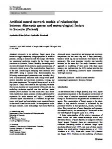
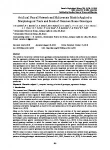
The model testing was conducted with all sales, covering the metropolitan areas of Adelaide as well as South Australian Regional centres and also within smaller micro locations. The smaller locations are based on suburbs. Adelaide has small suburbs with a few as 200 houses in some suburbs. Analysis at suburb level tends to remove any major locational factors from the analysis. All locations with 30 or more observations were chosen. This gave 30 suburbs in Adelaide. No regional centres had sufficient sales for effective model building. All thirty locations were used for the comparison of MRA models. Only three locations were chosen for the comparison of ANN models. This was due to the much greater time required for the analysis and greater complexity of model building tests. The locations used are indicated on location these is shown on Figure 1

Page 5

Page 6


Figure 1 - Location of Suburbs used in this Study

7

Reference Number

10 9

23

N

29

5 17

13 11 21

1

3 14 22 24 15 19 12 28 27 20 2 8 4 18 26 25 6

16

Reference

30 #

#

Used in MRA Models

Suburb

# of Cases

1

Brighton

44

2

Burnside

37

3

Campbelltown

30

4

Colonel Light Gardens

30

5

Enfield

53

6

Flagstaff Hill

37

7

Gawler East

36

8

Glen Osmond

33

9

Golden Grove

31

10

Greenwith

45

11

Henley Beach

48

12

Kensington Park/Gardens

55

13

Kidman/Flinders Park

36

14

Klemzig

35

15

Magill

37

16

Morphett Vale

31

17

Nailsworth

46

18

Netherby/Springfield

41

19

North Adelaide

48

20

Parkside

36

21

Plympton

36

22

Rostrevor

38

23

Salisbury

40

24

St. Peters

57

25

Stirling/Aldgate

35

26

Torrens Park

37

27

Unley

56

28

Wattle Park

46

29

West Lakes

35

30

Woodcroft

35

Used in MRA Models & in ANN Models

Variables

The variables used in the models are derived from either the DENR sales history file or the survey of households. For each location (and the whole State), models are produced in a step process; progressively add in a larger range of variables. This seeks to establish which variables are the key variables in modeling. Variables used from the DENR file were; Sale Price, Sale Date, Zone, Land Area, Equivalent Building Area, Building Condition Code, Year of Construction, Building Style, Wall Cladding and Roof Cladding, other Improvements. These variables relate primarily to the buildings with the exception of the land area and frontage. There is no qualitative site characteristics and no data regarding location, neighborhood characteristics, view or outlook. While much of this variation can be removed by modeling at suburb level, significant variations will still exist. Reasonable

Page 7


data on these issues can be collected from an inspection of the property from the road frontage. The following variables have been added to the data set through the student survey. 1. Site Characteristics - Slope, Hi-Low elevation, Aspect, Driveway Access 2. View Outlook - View distance, view angle, view type 3. Neighborhood - road size, street type, reserve location, streetscape, transmission lines, surrounding house quality, surrounding uses, location to public transport, shops and schools. 4. Subjective ratings - neighborhood, surrounding properties, house quality, site features, view/outlook, marketability, desirability. Prior to modeling, variables were re-coded where necessary. In order to enable regression modeling, a large number of categorical variables were re-coded to dummy variables. Dummy variables associated with the residential building were multiplied by the equivalent area to measure the effect on a per square metre basis rather than a single intercept basis. This has proven to be more effective in past modeling of Adelaide residential data. Price in raw dollar values was used as the dependent variable in all cases. Independent variables were added in the following steps Step

Variables Added

Comments

Step 1

Eq Area, Condition, Year of Construction

Basic DENR variables

Step 2

Eq Area, Condition, Year of Construction, Sales Date, ANN MODELS Zone, Land Area, ONLY All DENR Variables Style, Wall Cladding, Roof Cladding - as Categories

Step 3

Eq Area, Condition, Year of Construction, Sales Date, All DENR Variables Zone, Land Area, Style, Wall Cladding, Roof Cladding - as Dummies

Step 4

Eq Area, Condition, Year of Construction, Sales Date, All DENR Variables + Zone, Land Area, Subjective Ratings Style, Wall Cladding, Roof Cladding - as Dummies Subjective Ratings - neighborhood, Surrounding Properties, Streetscape, House Quality, Site Features, View, Marketability, Desirability

Step 5

Eq Area, Condition, Year of Construction, Sales Date, All DENR Variables + Zone, Land Area, Other Site, View and Style, Wall Cladding, Roof Cladding - as Dummies Neighborhood variables Site, View and Neighborhood Variables - Slope, Hi-Low, Aspect, Access, View distance, View Angle, View Type Dummies, Road Size, Street Type, Reserve, Public Transport, Schools, Shops, Streetscape, Transmission lines, Surrounding houses, Commercial uses.


Results Multiple Regression Models

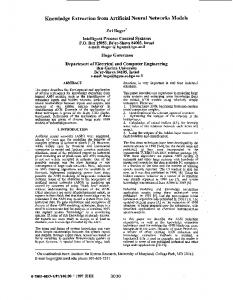
Multiple regression models form the basis of the automated valuation system being developed at the University of South Australia. These models are used to estimate adjustment factors which are applied to the most comparable properties in a grid adjustment method. The success of this automated system depends upon the ability to produce stable, robust price determinant models. The results from this research suggest that the DENR data currently being used, will produce such models but that further data is likely to enhance the predictive ability. The most basic models used in step 1 of the model building process produced highly stable robust models. Summarised output for this step is in Attachment 1. For each of the 30 locations, a significant model was produced by consideration of only the building area, condition and year of construction. The models are also remarkably consistent. All models included equivalent area. Most of the other models included either the condition code or year of construction or both. If condition or year of construction alone was added it was always positive. Models including both variables have a positive coefficient for condition code with a negative for year of construction. Addition of further variables from the DENR file usually leads to significantly better models. Relevant regression coefficients and statistics for steps 3 to 5 of the model building are shown in Attachment 2 to Attachment 4. Summarised results for each location and for a model using all the sales is shown in Table 1. The results in Table 1 show that the most significant increases in model explanation occur with the addition of equivalent area, condition and year of construction in step 1 and the remainder of the DENR variables in Step 3. Note that step 2 is not performed with MRA as this analysis can not deal with categorical variables. Most Suburbs have models with an adjusted R squared above .75 with the inclusion of the DENR data only. The most significant results for this research come in step 4 and step 5. In most cases the models improves with the addition of either the ratings variables in step 4 or the dummy and scaled variables in step 5. Overall the inclusion of the dummy and scaled variables is probably superior to the inclusion of the rating variables. At the end of the model building process in step 5, all models with the exception of Flagstaff Hill have an adjusted R squared above .7. Models for Flagstaff Hill, Glen Osmond and Nailsworth were poor prior to the inclusion of the final variables. These results would suggest that the DENR data is sufficient to build robust models in most locations but that the addition of the site, view and neighborhood variables can improve most models and will substantially improve the models in some locations.

Page 8

Page 9


Table 1 - Summarised Results for Regression Modles for 30 Suburbs and All Sales

Suburb

# of Cases 44 37 30 30

Brighton Burnside Campbelltown Colonel Light Gardens Enfield 53 Flagstaff Hill 37 Gawler East 36 Glen Osmond 33 Golden Grove 31 Greenwith 45 Henley Beach 48 Kensington 55 Park/Gdns Kidman/Flinders Park 36 Klemzig 35 Magill 37 Morphett Vale 31 Nailsworth 46 Netherby/Springfield 41 North Adelaide 48 Parkside 36 Plympton 36 Rostrevor 38 Salisbury 40 St. Peters 57 Stirling/Aldgate 35 Torrens Park 37 Unley 56 Wattle Park 46 West Lakes 35 Woodcroft 35 All Sales 1940

Adjusted R Squared F Value Step 1 Step 3 Step 4 Step 5 Step 1 Step 3 Step 4 Step 5 0.422 0.736 0.769 0.278

0.523 0.736 0.769 0.590

0.770 0.736 0.835 0.668

0.745 0.744 0.831 0.724

17 102 48 11

13 102 48 20

25 102 48 19

22 102 35 25

0.531 0.217 0.609 0.346 0.786 0.815 0.740 0.787

0.711 0.217 0.894 0.346 0.810 0.836 0.809 0.833

0.757 0.217 0.917 0.346 0.810 0.847 0.776 0.833

0.847 0.563 0.894 0.794 0.871 0.857 0.809 0.885

26 11 56 18 111 98 46 201

33 11 83 18 65 76 34 91

28 11 81 18 65 76 30 91

29 16 83 19 52 67 34 59

0.897 0.691 0.598 0.739 0.512 0.547 0.465 0.564 0.594 0.821 0.789 0.623 0.787 0.791 0.703 0.728 0.718 0.845 0.634

0.886 0.913 0.648 0.845 0.595 0.864 0.818 0.823 0.720 0.821 0.862 0.761 0.885 0.893 0.820 0.803 0.828 0.845 0.689

0.886 0.913 0.848 0.861 0.595 0.864 0.826 0.829 0.749 0.821 0.884 0.783 0.885 0.893 0.820 0.803 0.874 0.892 0.701

0.939 0.913 0.789 0.861 0.729 0.879 0.842 0.823 0.778 0.806 0.927 0.785 0.916 0.893 0.862 0.882 0.900 0.866 0.758

305 77 28 86 25 49 21 24 52 86 74 94 42 137 131 122 44 186 1120

235 88 47 56 23 52 36 41 31 86 62 46 52 61 62 62 56 186 266

235 88 35 56 23 52 33 42 27 86 91 41 52 61 62 62 48 95 215

93 88 28 56 25 49 28 41 32 74 71 41 61 61 67 68 52 111 236


Artificial Neural Network Models

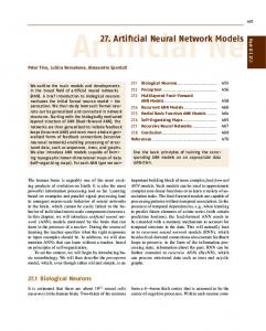
The ANN models produced were restricted to three suburbs and a model for all sales. This restriction was due to the time required to develop ANN models. The results are relatively consistent with those from the MRA modeling in regards the usefulness of the addition variables, but some further findings and comparisons are also possible. The models were built along similar lines to the MRA models. The major difference is the addition of the second step where categorical variables were included. ANN’s have some capabilities to deal with categorical variables however the ability of the network to cope a large number of categories is unclear. The mathematical preference is for numerical variables within a range of 0 to1 thus the conversion of a categorical variable to a number of dummy variables is likely to lead to more robust models which can produce better predictions, after less training. This is tested through steps 2 and 3. In step 2 the DENR data base was used with many variables in their native categorical state. In step 3 the DENR file is use but with the categorical variables converted to the dummy form that was used in the MRA Models. Steps 4 and 5 introduce additional data as in the MRA models. Thus steps 1,3,4 and 5 mirror those of the MRA models. For each step and for each location, two models were estimated; one using a fixed structure and one “optimised” using the genetic algorithm. Summarised results for all steps are shown in Table 2. The table shows some interesting patterns in the ability of ANN to form predictive models. There would appear to be real differences in the ability of ANN due to sample size. Rossini (1997b) suggested that ANN performed well for small data sets but had difficulty with larger data sets. This is also seem to be the case in this research and is highlighted in Table 2. The models using all sales (1940 observations) did not significantly improve over the process. In fact the addition of extra variables tended to cause lower predictive power in some cases. This may be due to stopping the learning process too early. However the shortest period of time given to any of the larger models was 12 hours of learning. While longer periods may have produced superior results, the time required makes this completely un-commercial in its application. Results from the larger all sales models suggest that the inclusion of the dummy variables at step 3 is superior to the categorical variables at step 2. This is supported by the results at suburban level. Generally speaking the optimised models performed slightly better than the standard models but there are models where they were inferior. The use of the optimisation algorithm seems to be most useful for larger data sets. The effect on the all sales models are quite significant and the effect at step 5 (were some 45 variables are used), is noticeable in all suburban models. The predictive ability of the models at different steps, closely follows the results from the MRA analysis. Initial models at step 1 are quite robust with a high degree of explanation with only three variables. By step 3 the models are generally good and at around an acceptable level for valuation practice. The inclusion of the additional site, view and neighborhood variables leads to an improved predictive power particularly at suburb level. As with the MRA models the effect varies depending upon the location. The more homogenous housing in Enfield allows for more simple models in both the MRA and ANN estimates than the more complex housing markets in inner city suburb of North

Page 10

Page 11


Adelaide or the beach side suburb of Brighton. In these more complex markets, view and neighborhood characteristics are more significant. Table 2 - Summarised Results for Neural Network Models - 3 Suburbs and All Sales - Step 1 to Step 5 Step 1

All sales All Sales Optimised Brighton Brighton Optimised Enfield Enfield Optimised North Adelaide North Adelaide Optimised

21.1% 22.1% 17.5% 18.0% 6.9% 6.2% 25.0% 28.6%

Step 2

29.3% 28.8% 8.4% 7.7% 2.6% 2.2% 11.7% 10.6%

Step 3

19.9% 18.3% 4.3% 3.3% 1.8% 3.5% 7.1% 5.8%

Step 4

24.9% 21.2% 3.9% 2.5% 3.8% 3.0% 5.80% 4.30%

Some General Finding about using ANN

During this research a number of further findings are worthy of some reporting. Two particular issues are the reporting of coefficients and the time issues of ANN’s. The non-linear nature of ANN’s makes it difficult to discuss the monetary effects of property characteristics. Unlike linear regression or log-linear regression where the coefficients have immediate meaning, the use of the sigmoid function and complex weighting systems in ANN’s makes simple interpretation very difficult. Several solutions exist to this problem. One such solution is to use the trained model to predict answers for a hypothetical set of observations where only one variables is changed. Table 3 shows one attempt at this. For each model at step one, predictions are done for hypothetical properties where in the first instance all variables are set at the minimum and in following instances each individual variable is set at its maximum. This estimates a range of price variation over the range of that variable. In Table 3 the total variation in the price of housing in Brighton which is due to equivalent area is estimated at $113,083, all other factors being equal. This equates to an average of $571 although this figure infers a linear relationship which is not true in the case of the sigmoid function. While these estimates are not true price adjusters, they do help to understand the behavior of the model.

Step 5

22.6% 17.1% 5.1% 2.0% 3.3% 1.5% 5.8% 3.3%

Page 12


Table 3 - Estimated Price Ranges and Average Prices based on ANN models at Step 1 Model

Eqarea (Range)

Eqarea (avg)

Condition (range)

Condition (avg)

Year Built (range)

Year Built (avg)

MAPE

All sales 3 (3,3,1)

$ 408,848

$ 507

$ 66,301

$ 9,472

-$ 14,094

-$

91 21.1%

All Sales 4(3,17,6,1)

$ 218,668

$ 271

$ 46,449

$ 6,636

-$

816

-$

5 22.1%

$ 113,038

$ 571

$141,436

$ 47,145

-$ 81,443

-$

1,163 17.5%

$ 111,053

$ 561

$128,468

$ 42,823

-$ 62,146

-$

888 18.0%

$ 18,232

$ 222

$ 3,828

$

957

$ 37,317

$

666

6.9%

$ 26,255

$ 320

$ 2,754

$

689

$ 13,027

$

233

6.2%

North Adelaide 3 (3,3,1)

$ 145,250

$ 183

$172,301

$ 34,460

$202,513

$

1,315 25.0%

North Adelaide Optimised 4(3,15,3,1)

$ 149,628

$ 189

$128,766

$ 25,753

$566,922

$

3,681 28.6%

Optimised

Brighton 3 (3,3,1) Brighton (3,10,1)

Optimised

3

Enfield 3 (3,3,1) Enfield Optimised (3,20,6,1)

4

The second issue is the time taken to build an ANN model. This is of particular relevance to the development of practical valuation systems. On a modern computer ( a Pentium 133 was used in these trials) an MRA model of nearly any practical size is estimated within seconds. ANN models take considerably longer. The most basic models estimated at step one with less than 50 observations would consume one to two minutes of computer time. The use of a genetic algorithm to establish an appropriate structure may increase this two or three fold. The suburban models using larger data sets at step 5 would normally require about 10 minutes of computer time; up to 30 minutes including the genetic algorithm. The larger models using all sales did not reach suitable learning stages after time periods which varied from 12 to 18 hours. At this stage the use of ANN’s for single residential valuations is probably a little too time consuming. An estimate for a single house based on recent sales would probably need to take less than two or three minutes to be viable. The suburban models are approaching this and with faster machines and better software will probably be there soon. Conclusions This research has helped to clarify several issues vital to the further development of automated and artificial intelligent valuation systems in South Australia. Many of the conclusions are likely to be relevant to other locations using other data sets. The data set currently available in South Australia through the Department of Environment and Natural Resources (DENR) is probably suitable for making reasonable price estimates of residential houses in most urban and suburban areas of South Australia. Models produced using either regression or ANN models should be suitable. Additional information which could be added to the DENR file would generally provide superior results moving most estimates from the reasonable to highly acceptable level and ensuring that a reasonable result is available in all locations. Additional variables which could easily be added by external examination and which would improve model capability would primarily relate to site characteristics, views and neighborhood qualities. Exactly which variables and in what form is not clear at this stage.


This research supports earlier work in South Australia (Rossini 1997a, 1997b) which suggests that either MRA or ANN’s could produce suitable models. Multiple regression models estimated over a range of suburbs suggest that this method would produce robust and stable results. This research did not seek to establish which was superior. However it would appear that MRA is superior for large data sets while ANN’s may be better for smaller data sets. This would support the use of ANN’s for valuation situations where micro-markets are examined in small neighborhood areas. The use of genetic algorithms to help determine ANN structures and key variables will lead to superior results particularly when using large data sets. Generally this research has helped to further the progress in the develop of automated and artificial intelligent valuation systems, particularly in South Australia.

References Baen, J.S & Guttery R.S. (1997) The Present and Potential Effects of Technology on the Property Professions in America, presented at the 3rd Pacific Rim Real Estate Society Conference, Massey University, Jan 1997 Borst, R.A and McCluskey (1996) The Role of Artificial Neural Networks in the Mass Appraisal of Real Estate, paper presented to the Third European Real Estate Society Conference, Belfast, June 26-28 Borst, R.A. (1991) Artificial Neural Networks: The Next Modeling/Calibration Technlogy for the Assessment Community? Property Tax Journal, IAAO, 10(1):69-94 Borst, R.A. (1995) Artificial neural networks in mass appraisal, Journal of Property Tax Assessment & Administration, 1(2):5-15 Detweiler J.H. and Radigan R.E. (1996) Computer-Assisted Real Estate Appraisal: A Tool for the Practicing Appraiser, The Appraisal Journal, January 1996, 91-101 Do, A.Q. and Grudnitiski, G. (1992), A Neural Network Approach to Residential Property Appraisal, The Real Estate Appraiser, Dec 1992:38-45 Eckert J.K., O’Connor P.M. and Chamberlain C (1993) “Computer-Assisted Real Estate Appraisal: A California Savings and Loan Case Study” The Appraisal Journal, October 1993, 524-532 Evans, A. James,H. And Collins, A. (1993), Artificial Neural Networks: an Application to Residential Valuation in the UK, Journal of Property Valuation & Investment: 11:195-204 James, H. And Lam, E, (1996) The Reliability of Artificial Neural Networks for Property Data Analysis, paper presented to the Third European Real Estate Society Conference, Belfast, June 26-28 Jensen, D.L. (1990) Artificial Intelligence in Computer-Assisted Mass Apraisal, Property Tax Journal, Vol 9, 5-26 Jensen, David L. (1984) Alternative Modeling Techniques in Computer-Assited Mass Appraisal, Appraisal Journal Kershaw, P.J. & Rossini, P.A. (1997a) Residential Time Series Analysis - An Automated Approach, Pacific Rim Real Estate Society Conference, New Zealand ,1997 Kershaw, P.J. (1997) Demonstrating Work on the School’s Expert Valuation System, Working Links Seminar September 1997, University of South Australia Kershaw, P.J., Rossini, P.A. & Kooymans, R.R (1996) Developing Specialised Software for Real Estate Applications A Case Study of the Development of Upmarket, 1st Pacific Rim Real Estate Society Conference, Brisbane ,1996

Page 13


Kershaw, P.J., Rossini, P.A. and Kooymans, R.R. (1994) UPmarket Software package REI South Australia. McCluskey, W.(1996a) Predictive Accuracy of Machine Learning Models for Mass Appraisal of Residential Property, New Zealand Valuer’s Journal, July:41-47 McCluskey, W., Dyson, K., McFall, D. & Anand,S. (1996b) Mass Appraisal for Property Taxation: An Artificial Intelligence Approach, Land Economics Review, Vol 2, No 1, 25-32 Nawawi, A.H., Jenkins D., Gronow S, (1997) Computer Assisted Rating Valuation of Commercial and Industrial Properties in Malaysia :- Developing an Expert System from a Multiple Experts Knowledge Elicitation Methodology paper presented to the Third European Real Estate Society Conference, Belfast, June 26-28 Rossini P.A. (1997a) Application of Artificial Neural Networks to the Valuation of Residential Property 3rd Pacific Rim Real Estate Society Conference, New Zealand ,1997 Rossini P.A.(1997b) Artificial Neural Networks versus Multiple Regression in the Valuation of Residential Property Australian Land Economics Review, November 1997 Vol 3 No 1 Rossini, P.A. Kershaw, P.J. & Kooymans, R.R. (1992) Micro-Computer Based Real Estate Decision nd Making and Information Management - An Integrated Approach 2 Australasian Real Estate Educators Conference Adelaide 1992. Rossini, P.A., Kershaw, P.J. and Kooymans, R.R. (1993) Direct Real Estate Analysis - The UPmarket™ Approach to Real Estate Decision Making, Third Australasian Real Estate Educators Conference, Sydney, 1993. Sauter, B. W. (1985) Valuation Stability: A Practical Look at the Problems, The Apppraisal Journal, ??? 243-250 Tay, D.P.H. and Ho, D.K.K. (1992), Artificial Inteligence and the Mass Appraisal of Residential Apartment, Journal of Property Valuation & Investment, 10:525-540 Tay, D.P.H. and Ho, D.K.K. (1994), Intelligent Mass Appraisal, Journal of Property Tas Assessment & Administration, Vol 1, No 1, 5-25 Worzala, E., Lenk, M. And Silva, (1995) A. An Exploration of Neural Networks and Its Application to Real Estate Valuation. The Journal of Real Estate Research, Vol. 10 No. 2

Peter Rossini, Lecturer - University of South Australia School of International Business North Terrace, Adelaide, Australia, 5000 Phone (61-8) 83020649 Fax (61-8) 83020512 Mobile 041 210 5583 E-mail [email protected]

Page 14

Page 15


Attachment 1 - Regression Analysis Step 1 Suburb # of Regression Coefficients Cases Eq Area Brighton Burnside Campbelltown Colonel Light Gardens Enfield Flagstaff Hill Gawler East Glen Osmond Golden Grove Greenwith Henley Beach Kensington Park/Gardens Kidman/Flinders Park Klemzig Magill Morphett Vale Nailsworth Netherby/Springfield North Adelaide Parkside Plympton Rostrevor Salisbury St. Peters Stirling/Aldgate Torrens Park Unley Wattle Park West Lakes Woodcroft All Sales

44 37 30 30 53 37 36 33 31 45 48 55 36 35 37 31 46 41 48 36 36 38 40 57 35 37 56 46 35 35 1940

F

Conditio Year n Built

$1,102 $19,680 $1,074 $446 $521 $1,122 $9,866 $280 $508 $670 $711 $696 $10,402 $749 $12,914 $1,326 $1,043 $1,186 $454 $567 $379 $1,443 $678 $816 $851 $672 $396 $1,092 $980 $1,704 $1,291 $1,127 $1,134 $597 $1,107

Adj Rsqd

$992 -$459

-$317

$382 $11,004 $37,194 $10,664 $1,123 $555 $18,001

-$960

$3,496 $13,651

-$920

0.422 0.736 0.769 0.278 0.531 0.217 0.609 0.346 0.786 0.815 0.740 0.787

16.80 101.60 47.50 11.40 25.90 10.90 55.50 17.90 111.00 97.90 45.50 200.60

0.897 304.60 0.691 76.80 0.598 27.70 0.739 85.70 0.512 24.60 0.547 49.30 0.465 21.40 0.564 23.60 0.594 52.20 0.821 85.80 0.789 74.00 0.623 93.60 0.787 41.60 0.791 137.20 0.703 131.00 0.728 121.70 0.718 44.40 0.845 186.40 0.634 1119.50

Page 16


Attachment 2 - Regression Analysis Step 3

Brighton

44 $1,082 $33,975

Burnside

37 $1,074

Campbelltown

30


30

Enfield

53

$905

Flagstaff Hill

37

$280

Gawler East

36

$677

Glen Osmond

33

$670

Golden Grove

31

$689

Greenwith

45

$582 $10,733

Henley Beach

48

$742 $12,031


55

$802 $14,211


36 $1,052

Klemzig

35

$518 $16,600

Magill

37

$431

Morphett Vale

31

$276

Nailsworth

46

$243 $13,587

$427,926


41

$587 $34,883

$1,476,132

North Adelaide

48

$713 $44,141

$2,364,759 -$527 -$360 -$467

Parkside

36

$701

$321

Plympton

36

$702

$321

Rostrevor

38

$672

$1,123

Salisbury

40

$301

$776

St. Peters

57

$867 $12,811

Stirling/Aldgate

35

$745

Torrens Park

37 $1,499

Unley

56

$348 $23,307

Wattle Park

46

$919

West Lakes

35 $1,203

Woodcroft

35

All Sales

$446

$761

Tudor

Stone

Date (per day)

nonreszone

Spanish

Colonial

Austerity

Bungalow

Contemporary

S.A.H.T.

Conventional

Villa

Cottage

Land Area (ha)

Timber Framed

Semi-Det

Year Built

# of Cases

Condition (Code)

Suburb

Eq Area (sq m)

Regression Coefficients

$0.0200

$992 $284 $9,314

$436,984

$316 -$418

$125 $164

$302,854 -$264

-$204

-$185

-$219

$816,254 $449,647

-$352

$596,709 -$475

1940 $1,229 $12,924

-$940 $24,981 -$274

$196,053 -$468 -$123 -$309 -$501 -$306 -$280 -$372 -$200 -$218 -$28,966

82.9

0.346

17.9

0.81

64.7

0.836

75.7

0.809

34

0.833

90.7

55.5 23.1

0.864

51.8

0.818

36.3

$148

0.823

40.6

$148

0.72

31.1

0.821

85.8

0.862

61.8

$0.0086 $313

0.761

45.5

$0.0120

0.885

51.6

$258

$597

10.9

0.894

0.595

$141 -$241

32.9

0.217

46.9

-$315

-$207

20.4

0.711

0.845

-$171

$1,629,873

47.5

0.59

0.648

$391

-$154

0.769

235

$352

$303

101.5

87.63

$121

$184,871

12.8

0.736

0.913

-$360

$453,986

F

0.523

0.886 -$334

$487

Adj Rsqd

$676

0.893

61

0.82

62.3

0.803

61.9

0.828

55.6

0.845

186.4

0.689

265.9

Page 17


Attachment 3 - Regression Analysis Step 4

44

Burnside

37 $1,074

Campbelltown

30

$358


30

$301

Enfield

53

$688

Flagstaff Hill

37

$280

Gawler East

36

$636

Glen Osmond

33

$670

Golden Grove

31

$688

Greenwith

45

$583 $10,733

Henley Beach

48

$766 $13,421


55

$803 $14,212


36 $1,052

Klemzig

35

$518 $16,601

Magill

37

$403

$526

Morphett Vale

31

$276

$487

Nailsworth

46

$243 $13,587

$427,926


41

$588 $34,883

$1,476,132

North Adelaide

48

$641 $39,932

$2,754,969 -$481 -$337 -$450

Parkside

36

$428 $14,989

Plympton

36

$684

Rostrevor

38

$672

Salisbury

40

$373

St. Peters

57

$838 $11,818

Stirling/Aldgate

35

$632

Torrens Park

37 $1,499

Unley

56

$348 $23,308

Wattle Park

46

$919

West Lakes

35 $1,188

Woodcroft

35

$1,235,804

$0.0014

$36,249

R-Prop

R-View

R-Site Features

R-Marketability

R-Streetscape

R-Neighbourhood

Tudor

Stone

Date

nonreszone

Spanish

Colonial

Austerity

Bungalow

Contemporary

S.A.H.T.

Conventional

Villa

Cottage

Brighton

All Sales

$501

Land Area

Timber Framed

Semi-Det

Year Built

# of Cases

Condition

Suburb

Eq Area


$27,326 $26,740

Adj Rsd 0.770

F 25.0

0.736 101.5 $981

$10,050 $204

$7,493

$445,201

$344

$7,256

-$426

$118

$10,374

$164 $302,854 -$311

$9,829 $816,254

0.835

48.3

0.668

19.1

0.757

28.0

0.217

11.0

0.917

81.1

0.346

17.9

0.810

64.7

0.847

75.7

0.776

29.6

0.833

90.7

0.886 235.0 $449,647 -$206

-$334 $310

0.913

87.6

0.848

34.6

0.861

55.5

0.595

23.0

0.864

51.9

$20,140

0.826

32.9

$18,070

0.829

42.0

0.749

27.1

0.821

85.8

0.884

91.0

$19,364

0.783

41.3

$16,632

0.885

51.9

0.893

61.0

$142

0.820

62.3

$258

0.803

61.9

0.874

48.3

0.892

94.9

-$208

$14,011

$121

$352

$391

$781,385 $326

$183

$14,478

$1,123 $7,228 $0.0008 $241 -$464

$180,100 $596,709 -$475

$241 -$154

-$208 -$1,087,893

-$220

$720

$20,910

$62 -$918 $24,413 -$197

$8,391

-$316

$1,629,873

$504

1940 $1,134 $12,022

-$119

$10,842

$133,714 -$416 -$103 -$278 -$395 -$270 -$227 -$326 -$193 -$209 -$26,176 $0.0002

$7,397 $7,930 $5,097 $3,958

0.701 215.3

Page 18


Attachment 4 - Regression Analysis - Step 5

Brighton Burnside

44

$862

37

$1,074

Campbelltown

30

$434


30

Enfield

53

Flagstaff Hill

37

$1,028

$677 $372

Golden Grove

31

$485

Greenwith

45

$549

$11,923

Henley Beach

48

$742

$12,032


55

$581

$16,742


36

$705

Klemzig

35

$518

37

$470

Morphett Vale

31

$276

Nailsworth

46

$213

$468

-$5,718

-$11,667

-$419 $501,530

$16,600

$1,044,805

Rostrevor

38

$663

$1,133

40

$320

$825

St. Peters

57

$866

Stirling/Aldgate

35

$608

$257,330

Torrens Park

37

$1,498

$596,709

$958

35

$568

1940

$1,130

Commercial Uses

Surrounding Houses

Powerlines

Street Trees

Shops

School

PubTransport

Reserve

Road Size

View - Rural

View-Greenspace

$15,218

-$42,091 $23,659

$21,780

$10,500

$14,053

$12,541 $340

$14,807

$294 -$322

-$43,408 $39,530

$93,894

-$387 -$11,337

-$104

$9,015

$14,839

$0.0092

$21,484

$8,245

$269

-$22,889 -$154

$6,223

$140

$30,239

$21,090

-$283

$233,973

-$341

-$225

-$17,171

-$463

35.4 24.6

0.847

29.3

$633

-$234

-$201

-$303

-$130

-$140

$102

$10,252

-$48,136

$14,290

16.4

0.894

82.9

0.794

18.6

0.871

51.6

0.857

67.0

0.809

34.1

0.885

59.2

0.939

93.1 87.6

0.789

27.8

0.861

55.6

0.729

25.2

0.879

49.3 28.3

0.823

40.6

0.778

31.7

0.806

73.8

0.785

41.2

$19,191

0.916

60.6

0.893

61.0

71.4

0.862

67.2

$36,400

0.882

68.2

$62,640

0.900

51.9

0.866

110.6

$5,576 -$740

101.5

0.927

-$37,203

-$158 -$270

$13,126

0.744 0.831 0.724

-$6,181

-$316

$1,514,742 $403,597

$16,150

$70,478

$333 -$475

21.9

0.842

$39,289

F

0.745

0.913

-$334

$310

Salisbury

$421

-$219

$285,430

$23,381

$1,162

$51,568

$11,380

$1,583,232

46

$54,445

$121

$13,330

Adj Rsd

0.563

$57,918

$649

$449,647

$3,036,730

35

-$32,694

-$280

$28,082

Wattle Park

$7,321 $16,735

-$265

$487

$37,261

West Lakes

-$186 $229

$476,250

$589

$412

-$10,514

-$7,698 -$205

$551

$921

$234 $152

$999,180

41 36

$62,227

$328,308 -$264

$8,588

$125

-$169

$500,840

48 36

View-Reserve $33,878 $9,633

Netherby/Springfield Parkside

View-Suburb

View-Ocean

View Distance

View Angle

Access

hi or low side

Slope

Tudor

Stone

Date (per day)

Spainish

Colonial

Austerity

Bungalow

Contemporary

S.A.H.T.

Conventional

$440,119

North Adelaide Plympton

$35,283

$31,950

$544

Magill

$22,762

-$9,689 $306

$7,923

36

All Sales

$99,153

$612

33

Woodcroft

$0.0140

$5,549

Gawler East

56

Villa

$1,072,424

Glen Osmond

Unley

Cottage

Land Area (ha)

Timber Framed

Semi-Det

Year Built

# of Cases

Condition

Suburb

Eq Area


$4,936

-$8,405