sensors Article
In Vivo Bioimpedance Spectroscopy Characterization of Healthy, Hemorrhagic and Ischemic Rabbit Brain within 10 Hz–1 MHz Lin Yang 1 , Wenbo Liu 2 , Rongqing Chen 1 , Ge Zhang 1 , Weichen Li 1 , Feng Fu 1, * and Xiuzhen Dong 1, * 1
2
*
Department of Biomedical Engineering, Fourth Military Medical University, Xi’an 710032, China;
[email protected] (L.Y.);
[email protected] (R.C.);
[email protected] (G.Z.);
[email protected] (W.L.) Department of Neurosurgery, Xijing hospital, Fourth Military Medical University, Xi’an 710032, China;
[email protected] Correspondence:
[email protected] (F.F.);
[email protected] (X.D.); Tel.: +86-29-8477-4846 (F.F.)
Academic Editor: Nicole Jaffrezic-Renault Received: 24 January 2017; Accepted: 4 April 2017; Published: 7 April 2017
Abstract: Acute stroke is a serious cerebrovascular disease and has been the second leading cause of death worldwide. Conventional diagnostic modalities for stroke, such as CT and MRI, may not be available in emergency settings. Hence, it is imperative to develop a portable tool to diagnose stroke in a timely manner. Since there are differences in impedance spectra between normal, hemorrhagic and ischemic brain tissues, multi-frequency electrical impedance tomography (MFEIT) shows great promise in detecting stroke. Measuring the impedance spectra of healthy, hemorrhagic and ischemic brain in vivo is crucial to the success of MFEIT. To our knowledge, no research has established hemorrhagic and ischemic brain models in the same animal and comprehensively measured the in vivo impedance spectra of healthy, hemorrhagic and ischemic brain within 10 Hz–1 MHz. In this study, the intracerebral hemorrhage and ischemic models were established in rabbits, and then the impedance spectra of healthy, hemorrhagic and ischemic brain were measured in vivo and compared. The results demonstrated that the impedance spectra differed significantly between healthy and stroke-affected brain (i.e., hemorrhagic or ischemic brain). Moreover, the rate of change in brain impedance following hemorrhagic and ischemic stroke with regard to frequency was distinct. These findings further validate the feasibility of using MFEIT to detect stroke and differentiate stroke types, and provide data supporting for future research. Keywords: brain impedance spectra; rabbits; stroke
1. Introduction Acute stroke, a serious and acute cerebrovascular disease, is classified into two clinical types: (1) hemorrhagic stroke, caused by blood bleeding into the brain tissue or the subarachnoid space through a ruptured intracranial vessel, which accounts for 13% of all stroke cases; and (2) ischemic stroke, caused by vascular occlusion in the brain due to a blood clot (thrombosis), which accounts for 87% of all stroke cases [1]. Stroke is characterized by sudden onset and high mortality and has been the second leading cause of death worldwide [2]. Prompt intervention improves the prognosis of stroke patients. Additionally, distinct interventions are needed for each stroke subtype. Hemorrhagic stroke patients require prompt surgical intervention, while ischemic stroke patients need thrombolytic therapy with tissue plasminogen activator within 3–4.5 h after the onset of stroke [3]. Hence, stroke should be
Sensors 2017, 17, 791; doi:10.3390/s17040791
www.mdpi.com/journal/sensors
Sensors 2017, 17, 791
2 of 16
typed to prevent the adverse effects of thrombolytic therapy on hemorrhagic stroke patients. Currently, CT and MRI are the main diagnostic tools used to diagnose stroke. However, in an emergency setting (e.g., in an ambulance), it is impractical to image the brain with CT or MRI [4]. Therefore, a portable tool that can detect stroke quickly under these circumstances is clearly needed. As a type of electrical impedance tomography (EIT), multi-frequency EIT (MFEIT) reconstructs the impedance distribution inside the human body according to the principle that the impedance of a biological tissue changes with frequency. In MFEIT, multi-frequency currents are simultaneously delivered through surface electrodes placed on the human body and the resulting boundary voltages are measured [5]. In this way, tissues are distinguished on basis of their specific impedance spectra [6]. Time-difference EIT (td-EIT) recovers the impedance change over time; but it is difficult to obtain data before disease onset in practice and thus td-EIT cannot be used to detect stroke [7]. Unlike td-EIT, MFEIT does not need any reference or baseline data acquired at other time points. Since there are difference in impedance spectra between normal, hemorrhagic and ischemic brain tissues [8], MFEIT shows promise in becoming an imaging modality that can quickly detect stroke and can also be used to identify stroke subtypes [4,9–11]. Previously, Yang et al. established brain hemorrhagic and ischemic models in rabbits and measured the impedance spectra of normal, hemorrhagic and ischemic brain tissues ex vivo [8]. These accurate tissue impedance spectral data form an important basis for stroke detection with MFEIT; however, these data may not fully reflect the features of impedance spectra of the healthy, hemorrhagic and ischemic brain when measured in vivo. Essentially, it is important to measure these features in vivo for MFEIT to be successful in detecting stroke, because MFEIT uses these features to image tissues [12,13]. In particular, the impedance spectra from the same animal species allow direct comparison of healthy, hemorrhagic and ischemic brain. To date, several research groups have investigated the impedance spectra of the healthy, hemorrhagic and ischemic brain. Lingwood et al. [14] and Ranck [15] measured the in vivo impedance spectra of healthy monkey (10 Hz–5 kHz) and rabbit (5 Hz–50 kHz) brains, respectively. Dowrick et al. made the measurement in vivo in healthy rabbit brains from 10 Hz to 3 kHz [16]. However, these studies did not establish animal models of hemorrhagic and ischemic brain, and measured their impedance spectra. In addition, these studies did not determine the impedance spectra at frequencies above 50 kHz (to improve the performance of MFEIT in detecting stroke, a frequency range of up to 1 MHz was suggested to be used [5,17]). In the case of ischemic brain, Dowrick et al. established an ischemic model in rats by occluding four vessels, and used four-electrode technique to measure the in vivo impedance spectra of the brain before and after ischemic stroke across the 1 Hz–3 kHz range [16]. Seoane et al. used four-electrode technique to determine the impedance spectra of the brain before and after hypoxia in neonatal and adult pigs across the 20–750 kHz range [18]. Wu et al. established an ischemic brain model in rabbits by ligating the carotid arteries, and used two-electrode technique to measure the impedance spectra of normal and ischemic brain across the 0.1 Hz–1 MHz range [19]. Other research groups monitored changes in impedance before and after brain ischemia at a single frequency [20,21]. Nevertheless, in these studies, the measurements of impedance spectra of hemorrhagic brain were not taken. Moreover, in the study by Wu et al., the two-electrode technique might affect the measurement results because of electrode contact impedance [16,22]. As for the hemorrhagic brain, several research groups monitored changes in the brain impedance before and after hemorrhagic stroke at a single frequency [20,23,24]. Seoane et al. measured and compared the impedance spectra of healthy and stroke-affected human brains across the 3.096–1000 kHz range [25]. However, these studies did not carried out the measurement of brain impedance within a wide frequency band (1 MHz). In the study by Seoane et al., because the results were obtained from different human subjects, the comparison of brain impedance before and after stroke was limited. In conclusion, although a number of existing publications have reported the impedance spectra of healthy, hemorrhagic and ischemic brain, the measurement results cannot be directly compared because of variations in experimental animals, modeling methods and
Sensors 2017, 17, 791
3 of 16
measuring conditions. Therefore, it is essential to establish hemorrhagic and ischemic brain models in the same animal species, and comprehensively measure and compare the impedance spectra of healthy, hemorrhagic and ischemic brain across the 10 Hz–1 MHz range. In this study, the intracerebral hemorrhage and ischemic models were established in rabbits, and the impedance spectra of healthy, hemorrhagic and ischemic brain were measured in vivo from 10 Hz to 1 MHz. Then, the difference in impedance spectra between healthy and stroke-affected brain was analyzed to assess the feasibility of using MFEIT to detect stroke, and difference in the rate of change of brain impedance between hemorrhagic and ischemic stroke with regard to frequency was also analyzed to identify stroke subtypes. Based on the results, the optimal frequency ranges for MFEIT to detect stroke and identify stroke subtypes were discussed. 2. Materials and Methods 2.1. Ethical Statement All animal experiments in this study were approved by the Ethics Committee for Animal Studies of the Fourth Military Medical University, Xi’an, Shaanxi, China. 2.2. Preparation of Animals Forty New Zealand rabbits (2.2 ± 0.3 kg), obtained from the Laboratory Animal Center of the Fourth Military Medical University, were divided into four groups: (1) hemorrhage group (n = 10); (2) hemorrhage control group (n = 10); (3) ischemia group (n = 10); and (4) ischemia control group (n = 10). Rabbits were deprived of food for 4 h and of water for 2 h before all experimental procedures. They were sedated by intraperitoneal injection of 1.5% pentobarbital sodium (2 mL/kg), followed by deep anesthesia by injecting 3% pentobarbital sodium (0.5 mL/kg) into the ear rim vein. During surgery, 1.5% pentobarbital sodium was injected intraperitoneally at a rate of 1 mL·kg−1 ·h−1 to keep the animal sedated. Animal body temperature was maintained at 39.5 ± 0.5 ◦ C with a warm water blanket and was measured with a rectal thermistor probe. Each animal was immobilized onto a stereotactic frame in a prone position by using eye- and ear-fixing bars. 2.3. Surgery Because stroke is primarily characterized by localized hemorrhage or ischemia, localized intracerebral hemorrhage and ischemic models were established. The hair on the rabbit’s head (approximately 15 cm2 ) was shaved with electric clippers. Then, the scalp and periosteum were removed with a scalpel; this was followed by electrocoagulation. Once hemostasis was achieved, the surgical field was cleared. The near-elliptical wound was approximately 3.6 cm long in the sagittal direction, and approximately 2.5 cm long in the coronal direction (Figure 1). To minimize water loss from the cranium and wound, an even layer of bone wax was smeared on the exposed cranium and an even layer of medical glue was smeared on the wound surface. 2.3.1. Intracerebral Hemorrhage Model The intracerebral hemorrhage model was established using autologous blood injection method [24]. The animal was immobilized onto the stereotactic frame and a hole was drilled with a dental bur 5 mm to the left of the sagittal suture and 5 mm behind the coronal suture. The hole was deep into the dura and was 1 mm in diameter (Figure 1a,c). Next, 1 mL of autologous blood was drawn from the heart and 0.4 mL of blood was aspirated into a 1-mL syringe. The syringe was fixed onto the stereotactic frame and the needle was inserted into the cranial hole. According to the anatomy of the rabbit brain, the needle was inserted at a depth of 11 mm to ensure that the blood was injected into the brain parenchyma. The injection of blood was started 1 min after the needle was inserted, and was completed within 2 min. The needle was withdrawn 30 min after completion of the injection. Finally, the rabbit was sacrificed by administering a pentobarbital overdose before the whole brain was taken
USA) was slowly injected into the ear rim vein at a dose of 1.5 mL/kg. When the rabbit’s eyes turned rose red (normally 15 min after the dye was injected), the LG150B-type cold light source (PhotoMachine Technological Exploration Corporation, Xi’an, Shaanxi, China) was turned on, and pure green light (wavelength: 540 nm; intensity: 600 mW/cm2) was transmitted via optical fibers. The probe (10 mm in diameter) connected to the optical fibers was placed perpendicular to the cranial hole,4 and Sensors 2017, 17, 791 of 16 the cranial hole was irradiated for 30 min. Finally, the rabbit was sacrificed by administrating a pentobarbital overdose and the whole brain was taken out to immerse in formaldehyde overnight for outh.toInimmerse in formaldehyde overnight for 24steps h. In the hemorrhage control all surgical steps 24 the ischemia control group, all surgical were the same as those group, in the ischemia group, were the same as those used for the hemorrhage group, except for the blood injection. except for green light irradiation.
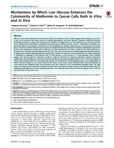
Figure intracerebral hemorrhage and ischemic models. (a) Schematic(a)diagram. (b) Figure 1.1. Localized Localized intracerebral hemorrhage and ischemic models. Schematic Electrode distribution for in vivo measurement of whole-brain impedance spectra. (c,d) Intracerebral diagram. (b) Electrode distribution for in vivo measurement of whole-brain impedance spectra. hemorrhage modelhemorrhage (autologousmodel blood(autologous injection method) and ischemic model (photochemical (c,d) Intracerebral blood injection method) and ischemic model induction method). (photochemical induction method).
2.3.2. Ischemic Model The ischemic model was established using photothrombotic stroke method [26]. A dental bur (10 mm in diameter) was used to drill the cranium 6 mm to the left of the sagittal suture and 5 mm behind the coronal suture through the outer plate layer to expose the inner plate layer, resulting in a 10-mm-wide round hole. Hemostasis was achieved by a gelatin sponge, and then the operating field was cleared (Figure 1a,d). Next, 3.5% rose bengal dye (Sigma-Aldrich Corporation, St Louis, MO, USA) was slowly injected into the ear rim vein at a dose of 1.5 mL/kg. When the rabbit’s eyes turned rose red (normally 15 min after the dye was injected), the LG150B-type cold light source (Photo-Machine Technological Exploration Corporation, Xi’an, Shaanxi, China) was turned on, and pure green light (wavelength: 540 nm; intensity: 600 mW/cm2 ) was transmitted via optical fibers. The probe (10 mm in diameter) connected to the optical fibers was placed perpendicular to the cranial hole, and the cranial hole was irradiated for 30 min. Finally, the rabbit was sacrificed by administrating a pentobarbital overdose and the whole brain was taken out to immerse in formaldehyde overnight for 24 h. In the ischemia control group, all surgical steps were the same as those in the ischemia group, except for green light irradiation.
Sensors 2017, 17, 791
5 of 16
2.4. In Vivo Measurement of Brain Impedance Spectra 2.4.1. Measurement: Protocol and Hardware Before establishing the intracerebral hemorrhage or ischemic model, six electrodes (copper nails, 0.93 mm in diameter; Hangzhou Westlake Biomaterial Corporation, Hangzhou, China) were placed onto the rabbit’s cranium. Two of the electrodes were placed along the sagittal suture, one 2 cm in front of and the other 1 cm behind the coronal suture, respectively. Two electrodes were placed on each side of the sagittal suture (0.8 cm away from the sagittal suture), the two electrodes on the same side being 0.8 cm apart in the sagittal direction. All electrodes were inserted approximately 1-mm deep to ensure that none of the copper nails penetrated the cranium. After all the electrodes were placed, they were further fixed onto the cranium with glue (DP100 epoxy adhesive; 3M Corporation, Maplewood, MN, USA; see Figure 1). The four-electrode technique was employed to minimize the effect of electrode contact impedance on the measurement. The two electrodes, located along the sagittal suture, were the exciting electrodes; the electrode in front of the coronal suture was the positive exciting electrode and that behind it was the negative exciting electrode. The electrodes on each side of the sagittal suture were the measuring electrodes; those in front of the coronal suture were the positive measuring electrodes and those behind it were the negative measuring electrodes. In the intracerebral hemorrhage group, the brain impedance spectra were measured 1 min after the needle was inserted, and the impedance spectra of post-hemorrhagic stroke were measured 30 min after blood was injected, i.e., 33 min after the needle was inserted. The time points used to measure the brain impedance were the same for the intracerebral hemorrhage group and its control group. In the ischemic model, the brain impedance spectra were measured before green light irradiation (15 min after injection of rose bengal dye) and 30 min after (45 min after injection of rose bengal dye). The time points used to measure brain impedance spectra in the ischemia group and its control group were the same. In this study, a Solartron 1260 impedance/gain-phase analyzer (Solartron Analytical, Farnborough, UK) with a 1294A impedance interface system was used to measure impedance, and the ZPlot software (Scribner Associates, Inc., Southern Pines, NC, USA) was utilized to control the acquisition of parameters. A 0.2 mA AC RMS signal was used across the two exciting electrodes to sweep from 10 Hz to 1 MHz in 51 steps. The voltage was measured by the two measuring electrodes and the impedance between the two measuring electrodes was calculated. In each measurement of brain impedance, when the measurement of the brain impedance spectra on one side was completed, the measuring electrodes were immediately replaced with the electrodes on the other side to continue the measurement. 2.4.2. Measurement in Saline Solution The four electrodes (two exciting electrodes and two measuring electrodes) were immersed into a beaker containing 0.03 M/L saline solution, and the impedance of the saline solution was recorded from 10 Hz to 1 MHz. Theoretically, the impedance of saline solution should not change with frequency [27]. Before each experiment, the impedance of saline solution was measured as the control. 2.5. Histopathology To evaluate the pathological changes of stroke-affected brain tissues, the animals were sacrificed with an overdose of pentobarbital sodium after the completion of the impedance measurement and their brains were taken out. In each group, the normal white and gray matter, and the hemorrhagic (the entire blood clot) and ischemic tissues (area surrounding the location of ischemia), all 1 cm in diameter, were removed from the brain and fixed in 10% formaldehyde for 24 h. After fixation, tissue specimens were cut into 3-mm thick sections, stained with hematoxylin and eosin and reviewed by a pathologist.
Sensors 2017, 17, 791
6 of 16
2.6. Data Analysis The impedance spectra of each side of the brain are denoted by ZL and ZR , respectively. The sum of the measurements of both sides (Z = ZL + ZR ) was used to investigate the impedance spectra of the whole brain. Because measurements were taken across a wide frequency range (10 Hz–1 MHz), the imaginary part of brain impedance was considered, and brain impedance was denoted by Z = Zreal + jZimag , where Zreal and Zimag are the real and imaginary part of brain impedance, respectively; j is the imaginary unit number and j2 = −1. For the four groups of animals, the brain impedance spectra were measured at two time points respectively denoted by before before after after Zbefore = Zreal + jZimag and Zafter = Zreal + jZimag , where Zbefore and Zafter were the first and second measurements respectively. When using MFEIT to detect stroke, the differential result of data at two different frequencies is preferred to eliminate common data errors, such as unknown boundary geometry and uncertainty regarding electrode position [7,10,28]. Therefore, it is important to know the relative change in brain impedance across the frequency range, rather than the absolute impedance. In this study, 10 Hz was used as the reference frequency to calculate the relative change in brain impedance across the 10 Hz–1 MHz range. First, to detect stroke with MFEIT, the healthy brain should be distinguished from the stroke-affected brain (whether ischemic or hemorrhagic). Hence, the difference ∆Z = ∆Zreal + j∆Zimag in brain impedance spectra between the healthy and stroke-affected brain was analyzed: after
before
∆Zreal = Zreal − Zreal after
(1)
before
∆Zimag = Zimag − Zimag
(2)
SPSS 22 (IBM Software, Armonk, NY, USA) was employed for the statistical analysis. The comparisons of brain impedance difference (∆Zreal and ∆Zimag ) at different frequencies between hemorrhage group and hemorrhage control group or between ischemia group and ischemia control group were carried out with one-way analysis of variance (ANOVA). The post-hoc test was used and p < 0.05 was deemed statistically significant. Second, when detecting the early stages of stroke, it is essential to discriminate the stroke subtype. Because MFEIT uses differences in tissue impedance spectra to image stroke, the difference in the rate of change of brain impedance with regard to frequency between hemorrhagic and ischemic stroke may be helpful to identify the type of stroke involved. In this study, because different surgeries were performed on rabbits to establish the intracerebral hemorrhage and ischemic models, it is meaningless to directly compare the impedance spectra of the ischemic and hemorrhagic brain. To address this issue, the whole frequency range was divided into three subranges and the lowest frequency was selected as the reference frequency in each subrange. The three frequency subranges were low (10 Hz–1 kHz; reference frequency: 10 Hz), intermediate (1 kHz–100 kHz; reference frequency: 1 kHz) and high (100 kHz–1 MHz; reference frequency: 100 kHz). For each subrange, the real and imaginary part of impedance spectra of ∆Z at the reference frequency were compared with those at the other frequencies to analyze the rate of change of ∆Z, as denoted by: f
ref
ref
f
ref
ref
(∆Zreal − ∆Zreal )/∆Zreal and (∆Zimag − ∆Zimag )/∆Zimag
(3)
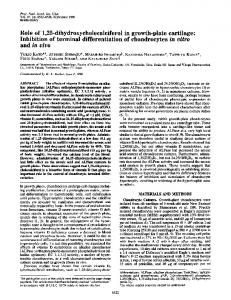
3. Results In all experiments, the animals had stable body temperature and respiration. Twenty sets of brain impedance spectra were obtained for each of the four study groups. As shown in Figure 2, the site of bleeding was in brain parenchyma (i.e., the white matter) in the intracerebral hemorrhage model and ischemia was mainly located in the cerebral cortex (i.e., the gray matter) in the ischemic model.
Sensors 2017, 17, 791 Sensors 2017, 17, 791
7 of 16 7 of 16
model. The volume of the blood clot was approximately 275 ± 25 mm3 in the intracerebral hemorrhage 3 inmm group; in theofischemia theapproximately ischemic tissue ± 0.3 in radius andhemorrhage 2.7 ± 0.25 mm in The volume the bloodgroup, clot was 275was ± 254.7mm the intracerebral group; thickness. in the ischemia group, the ischemic tissue was 4.7 ± 0.3 mm in radius and 2.7 ± 0.25 mm in thickness. Figure 2. (a) Intracerebral hemorrhage model; (b) Ischemic model. The arrow indicates the location of the stroke lesion.
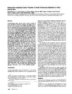
3.1. Measurement of the Impedance Spectra of Healthy, Hemorrhagic and Ischemic Brain As shown in Figure 3c, relative to the impedance at 10 Hz, the impedance change of the saline solution remained at nearly zero across the whole frequency range, indicating the reliability of our measurements. Figure 3a,b shows the real and imaginary parts of impedance spectra of the hemorrhage group and its control. From 10 Hz to 1 kHz, the real part of brain impedance decreased greatly and there was a local extreme point near 50 Hz for imaginary part. According to Schwan and Morowitz’s dispersion [29], 50 Hz should correspond to the characteristic frequency ofthe initial dispersion. Figure 2.theory (a) hemorrhage model; (b) Ischemic model. The arrow indicates location of (a) Intracerebral Intracerebral Figure 3c,d shows the changes in real and imaginary parts of brain impedance relative to the the stroke lesion. impedance at 10 Hz. Regarding the real part of brain impedance, there was a steep and nearly linear decrease (logarithmic frequency)Spectra of approximately 35%, from 10 to 200 Brain Hz. Between 200 Hz and 3.1. Measurement of the Impedance of Healthy, Hemorrhagic Ischemic Brain andHz Ischemic 1 MHz, the real part decreased slowly from −35 to −60%. The imaginary part of brain impedance As shown in Figure 3c, relative to the impedance at 10 Hz, the impedance change of the saline initially increased from 10 Hz to 100 Hz (a change of approximately 100%), then decreased within solution whole frequency range, indicating the the reliability of our solution remained remained atatnearly nearlyzero zeroacross acrossthe the whole frequency range, indicating reliability of 100 Hz–1 kHz (a change of 150%), and finally remained constant between 2 kHz and 1 MHz. measurements. our measurements. Figure 3a,b shows the real and imaginary parts of impedance spectra of the hemorrhage group and its control. From 10 Hz to 1 kHz, the real part of brain impedance decreased greatly and there was a local extreme point near 50 Hz for imaginary part. According to Schwan and Morowitz’s dispersion theory [29], 50 Hz should correspond to the characteristic frequency of initial dispersion. Figure 3c,d shows the changes in real and imaginary parts of brain impedance relative to the impedance at 10 Hz. Regarding the real part of brain impedance, there was a steep and nearly linear decrease (logarithmic frequency) of approximately 35%, from 10 Hz to 200 Hz. Between 200 Hz and 1 MHz, the real part decreased slowly from −35 to −60%. The imaginary part of brain impedance initially increased from 10 Hz to 100 Hz (a change of approximately 100%), then decreased within 100 Hz–1 kHz (a change of 150%), and finally remained constant between 2 kHz and 1 MHz. Sensors 2017, 17, 791
8 of 16
Figure3.3. The The brain brain impedance impedance spectra spectra of of the the intracerebral intracerebral hemorrhage hemorrhage group group and and its its control control group. group. Figure (a,b)Real Realand andimaginary imaginaryparts partsof ofbrain brainimpedance impedancespectra; spectra;(c,d) (c,d)The Thechanges changesin in the the real real and and imaginary imaginary (a,b) partsof ofbrain brainimpedance impedancerelative relativeto tothe theimpedance impedanceatat10 10Hz. Hz. parts
Figure 4a,b shows the real and imaginary parts of the brain impedance spectra of the ischemia Figure 3a,b shows the real and imaginary parts of impedance spectra of the hemorrhage group group and its control. The magnitude of real and imaginary parts after ischemic stroke was greater and its control. From 10 Hz to 1 kHz, the real part of brain impedance decreased greatly and there was than that recorded before stroke. Figure 4c,d shows the changes in the real and imaginary parts of the brain impedance spectra relative to the impedance at 10 Hz. The magnitude and trend of changes in the real and imaginary parts for the ischemia group and its control were like those for the hemorrhage group and its control.
Sensors 2017, 17, 791
8 of 16
a local extreme point near 50 Hz for imaginary part. According to Schwan and Morowitz’s dispersion theory [29], 50 Hz should correspond to the characteristic frequency of initial dispersion. Figure 3c,d shows the changes in real and imaginary parts of brain impedance relative to the impedance at 10 Hz. Regarding the real part of brain impedance, there was a steep and nearly linear decrease (logarithmic Figure 3. The brain impedance spectra of the intracerebral hemorrhage group and its control group. frequency) of approximately 35%, from 10 Hz to 200 Hz. Between 200 Hz and 1 MHz, the real part (a,b) Real and imaginary parts of brain impedance spectra; (c,d) The changes in the real and imaginary decreased slowly from −35 to −60%. The imaginary part of brain impedance initially increased from parts of brain impedance relative to the impedance at 10 Hz. 10 Hz to 100 Hz (a change of approximately 100%), then decreased within 100 Hz–1 kHz (a change of 150%), and finally remained constant between 2 kHz and 1 MHz. Figure 4a,b shows the real and imaginary parts of the brain impedance spectra of the ischemia Figure 4a,b shows the real and imaginary parts of the brain impedance spectra of the ischemia group and its control. The magnitude of real and imaginary parts after ischemic stroke was greater group and its control. The magnitude of real and imaginary parts after ischemic stroke was greater than that recorded before stroke. Figure 4c,d shows the changes in the real and imaginary parts of than that recorded before stroke. Figure 4c,d shows the changes in the real and imaginary parts of the the brain impedance spectra relative to the impedance at 10 Hz. The magnitude and trend of changes brain impedance spectra relative to the impedance at 10 Hz. The magnitude and trend of changes in in the real and imaginary parts for the ischemia group and its control were like those for the the real and imaginary parts for the ischemia group and its control were like those for the hemorrhage hemorrhage group and its control. group and its control.
Figure Figure 4. 4. The The brain brain impedance impedance spectra spectra of of the the ischemia ischemia group group and and its its control. control. (a,b) (a,b) The The real real and and imaginary imaginary parts parts of of the the impedance impedance spectra; spectra; (c,d) (c,d) The The changes changes in in the the real real and and imaginary imaginary parts parts of of brain brain impedance impedance relative relative to to the the impedance impedance at at10 10Hz. Hz.
3.2. 3.2. Difference Difference in in Impedance Impedance Spectra Spectra between between Healthy Healthy and and Stroke-Affected Stroke-Affected Brains Brains (Hemorrhagic (Hemorrhagicor or Ischemic Ischemic Brain) Brain) Figure Figure 5a,b 5a,b shows shows the the differences differences in in real real and and imaginary imaginary parts parts of of brain brain impedance impedance spectra spectra in in the the hemorrhagic hemorrhagic group group (measured (measured before before and and after after blood blood was was injected) injected) and and its its control control (measured (measured 11 min min and 33 min after the needle was inserted). As shown in Figure 5a, the difference in the real part before and after blood was injected decreased initially from 10 Hz to 100 Hz and then increased within 100 Hz–1 MHz, varying in the range from 6.4 ohms (smallest value at 100 Hz) to 11.3 ohms (largest value at 1 MHz). In contrast, the difference in the real part was less than six ohms in the hemorrhage control group. Across the whole frequency range, there were significant differences in the real part between the hemorrhage group and its control (p < 0.01). In the hemorrhage group, the difference
imaginary part differed significantly between the hemorrhage group and its control (p < 0.05). These results indicated that brain impedance spectra changed significantly following hemorrhagic stroke. Figure 5c,d shows the differences in real and imaginary parts of brain impedance spectra in the ischemia group (measured before and after irradiation with green cold light) and its control group (measured 15 min and 45 min after the injection of rose bengal dye). In Figure 5c, the difference in Sensors 2017, 17, 791 9 of 16 the real part before and after irradiation with green cold light changed slowly from 10 Hz to 500 Hz and then decreased significantly from 500 Hz to 1 MHz, with difference greater than four ohms across the whole frequency The sharply difference real from part in group was significantly in the imaginary partrange. increased byin 5.3the ohms 10the Hzhemorrhage to 500 Hz, declined slowly by one larger than those in its control group (p