Catching Up or Falling Behind? Income Distribution of Chinese Cities Chun-Yu Ho1
Dan Li2*
Boston University First Version: November 2005 Second Version: July 2006 Current Version: March 2007
Abstract This paper analyzes the evolution of Chinese urban income distribution across space and time in post-reform era. Our results suggest no evidence on income convergence across cities during the period 1984-2003. We find that cities with comparable income level are likely to be co-located in the same region; further, cities tend to mirror the mobility of their counterparts located in the same province, but not the same region. The divergence in urban income across the nation will continue if the current economic growth pattern persists in the future. JEL classification: O15, O18, R12, R58 Keywords: City Income Distribution; Convergence; Markov Process; Spatial Dependence; China
1
Email:
[email protected]; URL: http://people.bu.edu/chunyu; Address: Department of Economics, Boston University, 270 Bay State Road, Boston, MA 02215. 2 Email:
[email protected]; URL: http://people.bu.edu/danli; Address: Department of Economics, Boston University, 270 Bay State Road, Boston, MA 02215. *Corresponding author. Tel.: +1 617 353 3743.
1
1. Introduction The process of urbanization in developed economies has long been a focus of economic research but the process in developing countries has been much less studied (Williamson, 1965; Henderson, 2002). In this paper we examine a key feature of urbanization in contemporary China, a country that is undergoing both rapid economic development and city growth: differences in per capita income across cities and their evolution over time from the beginnings of “reform” (1984) to the latest year for which data are available (2003) when our study was first conducted. Our basic finding is simply put – there is no evidence of income convergence across Chinese cities over this period. Instead, we find a persistent component of similarity in incomes controlling for province (and, hence, for region); it is as if Chinese cities have a pre-determined steady state level of per capita income conditional on their location (province).
These patterns are clearly consistent with
some models of the growth process but not others, and they also suggest that regional disparities in economic performance, already very prominent, may continue as the Chinese economies grows further in the 21st century. Our results complement those of other scholars of China’s recent urban history, including Anderson and Ge (2005) who focus on the evolution of the city size distribution over the second half of the twentieth century. In the next section, we briefly explain the theoretical background to our study and why China is an interesting application of the theory. Section 3 discusses the data, section 4 our econometric approach, and section 5 presents our results. Concluding remarks are presented in the final section.
2. Theoretical background and the case of China According to the Solow growth model, differences in per capita incomes across economies should converge, in the sense that economies with a high initial income should grow more slowly than economies with a low initial income. As is well known, the underlying reason for convergence is diminish returns to capital -- where capital intensity is low, incomes are low, and the returns to capital are high; conversely, if 2
capital intensity is high. Consequently, capital accumulation should be more rapid in economies with low initial income, which results in more rapid growth, and hence convergence. A problem with the Solow growth model is that much of the world fails to exhibit convergence – or, at best, presents a mixed picture (Barro 1991; Quah 1993a, b). A variety of explanations have been suggested for the mixed record of success of the model. Gallop et al. (1999) asset that location and climate have significant effects on growth by affecting transportation cost, disease burden and agricultural productivity. In this case, one would predict “conditional convergence” – countries will converge to the same steady state level of per capita income only if they share the same “fundamentals”.
Still another approach is to relax the assumption of diminishing
returns to capital by assuming technology spillovers (Romer, 1986) or endogenous human capital accumulation (Lucas, 1988; Mankiw et al, 1992); with endogenous growth, economies may fail to converge even if they share similar characteristics, such as climate. Many researchers have empirically tested the convergence theory using various methodologies. In addition to the cross country analysis in Barro (1991) and Quah (1993a, b), researchers examine regional convergence at state level3 and sub-state level.4 In particular, the empirical results from the sub-state level show a mixed picture for convergence. Although many studies of convergence have been conducted using cross-country data, regional (or other geographic) variation within large countries provides a useful source of information. In this regard, China is of particular interest for two reasons. First, and foremost, China has an enormous population; if there are persistent differences in per capita income within the country, the overall consequences for human welfare are much greater than, say, for other large, but less populous countries (e.g. Canada). Second, there are significant differences in climate, access to water 3
Magrini (2004) provides an excellent review. There are many studies using provincial data in China to study convergence. In addition to studies employing Barro-type regression, the studies using distribution approach include Bhalla et al (2003), Li (2003) and Sakamoto and Islam (2006). 4 For evidences of convergence at city level: Glaeser et al (1995) and Crihfield and Panggabean (1995) for U.S.; Jones et al (2003) for China.
3
transportation, topography, and other features of the environment that create a “natural experiment” for exploring the effects of geography on convergence. For example, western China is landlocked; and it has low agricultural productivity due to a cold and arid climate, and limited access to irrigation from the Yangtze and Yellow Rivers.5 Recent patterns of convergence in China may have been affected by the actions of the central government. In particular, China underwent a series of economic “reforms” in three stages: 1978-84, 1985-91, and 1992-present. Deng Xiaoping came into power after the Third Plenary Session of the Eleventh Chinese Communist Party Congress in December 1978. The first stage of the reform began with the so-called “household responsibility system” that linked remuneration to output for agricultural production, and which led to a substantial rise in agricultural productivity, a necessary condition for urban growth (Papageorgiou and Smith, 1983). In addition, four special economic zones (SEZs)6 were established to attract foreign direct investment during the first stage of reform.7 During the second stage, the government included stateowned enterprises (SOEs) into the reform agenda. Compared with traditional state owned enterprises, SOE’s were allowed to retain extra profits after fulfilling the contracted quota and have control over personnel decisions. Other changes during the second phase included improved managerial incentives, a stock market, and tax reform, and the elimination of the so-called “dual-track” pricing system in the early 1990s.8 Deng Xiaoping’s speech during a visit to southern China in 1992 ushered in the third stage of reform – a widespread opening up of markets and a commitment to a market economy. The third phase also included a plan to develop Western China, 5 The altitude of Qinghai-Tibet Plateau in the west is about 4000m high and then it gradually decreases to less than 1000m plains in the east. Thus, the weather in the west is colder than that in the east. Huang (1997) argues that farming concentrates on the east of the 14 inches (356 mm) isohyets which divide China into temperate (northwestern part of China) and tropical zones. 6 The SEZs were set up in the cities of Shenzhen, Zhuhai and Shantou in Guangdong province in 1980 and Xiamen in Fujian province in 1981. 7 However, FDI inflow did not increase until 1984. In the same year, the Chinese government decided to open other 14 coastal cities and Hainan island (which became a province in 1988). A detailed timeline of preferential policy in China can be found in Demurger et al (2002). 8 In July of 1984, the first shareholding company, Beijing Tianqiao department store (shareholding), was formed. In 1991, at the end of the second stage of reform, there were 709 SOEs restructured to the shareholding system. SOEs paid taxes on their revenue to state and local governments instead of handing in profit. This policy aimed to loose the relation between SOE and local authorities. Some goods and services were allocated at state controlled prices, while others were allocated at market prices.
4
although the central government’s ability to do so may have been hampered by a reduction in its share of total government revenue. To summarize, the Chinese economy has grown rapidly since the onset of economic reform in the late 1970s. Because China is a large country with an extremely diverse topography and climate, there are good reasons to believe that convergence, if it is observed, will be conditional rather than absolute (as in the original Solow growth model). Additional variation in the regional growth process has been introduced by conscious policies taken by the central government that vary over time, depending on the state of the reform. Consequently, China offers a unique internal laboratory for examining the convergence process, one that is almost with parallel in the world today.
2. Data We analyze the spatial evolution of per capita GDP in urban areas in China during five sub-periods: 1984-1987,9 1987-1991, 1991-1995, 1995-1999, and 1999-2003. Our data come from various issues of Chinese Urban Statistics Yearbooks published by China’s State Statistical Bureau. It is well known that per capita GDP may not be a perfect proxy for income -- in particular, when there are remittances from one city to another; or dividends that are earned in one city but paid to residents elsewhere; and, of course, profits of foreign-owned companies. However, to the best of our knowledge, there is no alternative to using per capita GDP prior to 1990, and thus we follow the previous literature in focusing on this variable.10 Before beginning our econometric analysis it is useful to provide a brief description of the administrative structure (see Figure 1) in mainland China. The mainland is divided into 27 provinces and 4 municipalities, which are the first administrative level. Beginning in 1983, the government implemented a new administrative format setting up the “prefectural-level city” (the second level) by assigning adjacent rural counties (the third level) to be under the city’s 9
For this period, there is only four-year interval compared to the five years for the later periods because the data for 1983 are not available. 10 See Magrini (2004).
5
administration.11As urbanization progresses some rural counties became “county-level cities” (also at the third level); however, they are still under the prefectural-level government administration. Below the county, there are towns, which belong to the lowest level. Because of this structure, “cites” in Chinese terminology do not only refer to the urban areas12 since rural counties and towns are attached to them. In the yearbooks, information on own urban area (Shiqu)13 and the overall administrated territory (Diqu) are available for prefectural-level cities and municipalities. After the total number of cities increased from 300 in 1984 to 660 in 2003, the city yearbooks do not record information on county-level cities since 1991. Hereafter, city is used interchangeably with the urban area (Shiqu), which is the focus of our study. In order to maintain a large sample size, we include the county-level cities into our sample in the first sub period (1984-1987) since more than 95% of the county-level cities in 1984 evolved to the prefectural-level cities in 2003. However, owing to the data limitation for the county-level cities in the later years, we are forced to focus on the urban area of the cities at the prefectural-level and above.14 All data reported for a given year refer to economic activity during the previous calendar year (for example, the 2004 yearbook includes data for the calendar year 2003. Urban per capita GDP is directly available for years 1991, 1995 and 2003. For 1999, it is obtained by dividing GDP by registered urban residents. Since total urban GDP is not available for 1984 and 1987, we use industrial GDP as a proxy for it.15 Table 1 provides descriptive statistics for our dataset. We divide mainland China into three regions: Eastern, Central and Western, where Eastern region has eight provinces 11
Not all the rural counties are under the city’s administration. Especially, some counties consist of minorities (non-Han Chinese) and they are self-governed and so-called autonomous counties. 12 In Anderson and Ge (2005), they state that the “this “city proper” definition may only represent a “traditional” downtown area and exclude suburbs”. We think this statement might only be correct for a very few “urban proper” for county-level cities and urban areas of most large “cities” were expanded and many multi-centered cities emerged. 13 It excludes their lower-level cities’ (county-level cities’) urban area. 14 The urban area of most county-level cities in 2003 is small and informal, with the metropolitan area being not well defined, since they evolve from a very small rural county. Thus, we believe that the exclusion of the urban area of these cities will not affect our results on the urban growth to a significant extent. 15 China started the reform in urban area during the period 1984-1987, with the tertiary industry contributes a tiny fraction of the city GDP relative to that of industrial GDP. Hence, industrial GDP captures most part of overall GDP.
6
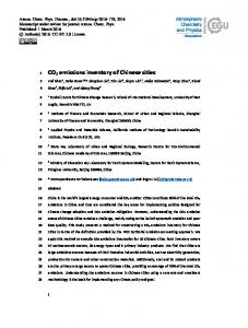
and three municipalities, Central has seven provinces and one municipality, and Western region has twelve (see figure 3).16 Figure 2 shows the kernel densities of the urban income distribution in our sample years. It shows that the kernel density in 2003 has a similar shape as that in 1984. We have standardized the distributions at zero and it clear that, since 1987, there is more clustering around at zero, which is suggestive of convergence. However, while the kernel densities are informative, they do not reveal intra-distributional mobility along the urban income hierarchy.
4. Methodology In this section, we briefly describe the methodologies used to investigate the dynamics in the cross-section and time-series of city incomes. We first employ Markov transition probability matrix in Quah (1993a) to uncover the transitional dynamics over time. Then, indices in Quah (1997) and Rey (2004) are used to explore static and dynamic spatial dependence.
4.1 Markov chain and the derived indices A Markov chain is employed to map the income distribution from one period to another: Pt + s = Pt M
t ,t + s
(1)
where Pt is a 1×K probability distribution vector that summarizes the distribution in period t, and Pt+s in period t + s. Matrix Mt,t+s describes the evolution of the distribution over period s as follows.
M t ,t +s
⎛ m11 " m1 j " m1K ⎞ ⎜ ⎟ # # ⎟ ⎜ # = ⎜ mi1 " mij " miK ⎟ ⎜ ⎟ # # ⎟ ⎜ # ⎜m ⎟ ⎝ K1 " mKj " mKK ⎠
(2)
16
The regional division of mainland China in our paper does not strictly follow the geographic location (figure 3). Western region includes 12 provinces, which were selected into the Plan of Western Region Development launched by China government in 1999.
7
where mij is the probability of a city making a transition from income class i to j over time s. We standardize the city per capita GDP by subtracting sample means and, then dividing it by standard deviation. Then, the space of standardized values is discretized into K=4 intervals at {≤-0.5, (-0.5, 0], (0, 0.5], >0.5}, denoted class 1, 2, 3 and 4.17 In our study, the number of observations in the four classes are close to each other, thus the grids chosen approximate the underlying distribution reasonably well. The off-diagonal entries in Mt,t+s record the distributional dynamics with larger values implying more mobility. Conversely, the diagonal entries trace persistence, that is whether rich cities remain rich or poor cities remain poor over time. In order to ease the comparison of different transition matrices across time and space, Shorrock’s (1978) index is used to summarize the extent of persistence. SI t ,t +s =
K − Tr (M t ,t +s ) K −1
(3)
where Tr indicates the trace operator. This index is bounded on [0, 1.33] for a transition matrix with 4 intervals. Lower values reflect more persistence (less mobility) across income states over time. To examine the long term outcome of current growth patterns, we compute the steady state distribution, where individual cities move up or down the income ladder in a way that preserves the distribution. If the Markov chain is ergodic, we get the steady state P* = lim Pt M t ,t +n by iterating the transition matrix n time. n→∞
4.2 Static spatial dependence The phenomenon that the rich tend to neighbor with the rich and poor cluster with the poor is commonly observed in an economy, which is called spatial dependence/conditioning (Quah, 1993b). At a point of time, we compute both the standardized income distributions with respect to the regional average and the national average for comparison. From the two series, we construct a matrix to represent a 17
The discretization is important for a Markov chain to approximate the unobserved density function. More classes improve the approximation but reduce the number of observations in each class and hence the accuracy of the transition matrix. On the other hand, fewer classes discard information on the intra-distributional dynamics, especially for the upper and lower tails.
8
degree of correspondence between the positions of a city in each conditional distribution. A K×K matrix SA,N is constructed as follows:
S A ,N
⎛ s A 1, N 1 ... s A 1, N j ... s A 1, N K ⎜ # # ⎜# ⎜ = s A i , N 1 ... s A i , N i .... s A i , N K ⎜ ⎜# # # ⎜⎜ ⎝ s A K , N 1 .. s A K , N j .... s A K , N K
⎞ ⎟ ⎟ ⎟ ⎟ ⎟ ⎟⎟ ⎠
(4)
where sAi,Nj is the probability of a city belong to income class i in region A and fall in class j in nation N in a year. If city incomes are randomly distributed in space, the transitional matrix should be largely diagonal because each city should belong to a similar class in the region as well as the nation. Rey (2004) suggests a trace statistic ζ =1−
K
∑
s A i , N i to examine whether the joint probability matrix departs from
i =1
diagonal matrix. The statistic ranges from 0 to 1 with higher value implying more spatial dependence in city incomes.
4.3 Dynamic spatial dependence The trace statistic in the previous section reflects the static nature of spatial dependence. Rey (2004) introduces a measure to investigate dynamic spatial dependence; that is, whether strong growth cities tend to neighbor with each other. It is implemented by computing a scalar measure, the Spatial Clustering Index (SCI), as follows: ψ
t ,t + s
=
∑ ∑ ∑ θ
i∈ A
A
i
θ i ,t + s − θ i ,t
i ,t + s
− θ i ,t
(5)
where θi ,t represents the rank of income of city i among all cities in our sample in year t and θi ,t + s in year t+s. The rank difference of city i between two periods implies whether the income growth is in tandem with, lagged behind or overtakes her counterparts over time s. A in equation (5) is one of a set of exhaustive and mutually
9
exclusive groups of cities. For instance, A can be a group of cities in a province or a region composed of several provinces.18 The denominator is the sum of the absolute rank changes over time. This measure should be close to 1 if the movement in income distribution is cohesive within areas. It approaches zero if the cities in a pre-defined area are moving in different directions in the distribution.
5. Empirical results and interpretations 5.1 Distributional dynamics We begin by examining transition matrices at both the national and regional levels over the 19 year time spans shown in Table 2. In 1984, there were 85 and 88 cities, respectively, in the eastern and central regions compared with 54 cities in the western region. Further, the eastern region has a high concentration of high-income-level cities and low concentration of class 1 cities (poorest cities). For example, amongst the 54 wealthiest cities in 1984, 63 percent are located in the east, 28 percent in the central and only 9 percent in the west. In contrast, only 18 out of 85 cities in the eastern region fall into class 1, whereas 35 out of 88 in the central and 27 out of 54 in the west. Table 2 shows there is a 50 percent probability for cities in class 1 in 1984 moving up to higher classes in the east, compared with 35 percent in the central region and 24 percent in the west. In contrast, the richest cities in the east have 71 percent probability to remain in the fourth class, compared with 33 percent and 20 percent for those in the center and west, respectively. For middle-class cities at the beginning point, those in the eastern region have equal probability to move up or down; those in the central and west are more likely to degrade. By the end of 2003, 34 out of the 49 wealthiest cities fell in the east (70 percent), 11 in the center (22 percent) versus 4 in the west (8 percent). On the other hand, 21% (18/85) cities in the eastern fall in class 1, 40% (35/88) for the center and 50% (27/54) for the west. These results indicate that cities in the initial wealthy eastern region gain favorable upward moves in the national 18 Hammond (2004) uses this index to analyze the spatial pattern of income growth across metropolitan and non-metropolitan areas in U.S.
10
income ladder, at the expense of both its central and western counterparts over the last two decades. The pattern of regional income evolution can be partially explained by institutional and geographic factors. After 1984, Special Economic zones/districts and Open Economic cities were established in the eastern region. The status of the special treated regions were further enhanced by a 1986 law that gave certain privileges to foreign joint ventures, such as preferential tax treatment, and various rights to import inputs and engage in foreign exchange operations. 19 The Eastern coastal areas proximity to ocean transport and, in particular, to Hong Kong lowered transaction costs for international trade (Bao et al, 2002). Consequently, output in the coastal areas rose rapidly due to the huge foreign investment. The institutional changes from planned to market economy also benefited the coastal areas relatively more because, prior to reform, there were in these areas relatively fewer state enterprises initially; there was, in other words, more economic “space” within which smaller, private-sector enterprises could thrive (Bai et al, 2003).20 On the other hand, the cities located in the inland experienced less economic growth than their coastal counterparts. Fan and Chan-Kang (2005) show that, during the past two decades, the difference in economic growth rates between the coastal and inland regions was as high as 3 percentage points. In addition to less favorable economic policies, poor physical and social infrastructures and the remoteness from the seaport, fiscal decentralization worsened the ability of the central government to finance the inland government spending. Zhang and Zou (1998) find a negative relationship between fiscal decentralization and economic growth in the inland China. Furthermore, the household registration system in China restricts the inland people move away from their birth cities to more economically prosperous cities in the 19
See the provisions of the State Council of the People’s Republic of China for the Encouragement of Foreign Investment. 20 For example, the development model of Wenzhou in Zhejing Province involves mainly small enterprises in light industries. Sonobe et al (2004) document that firms in Wenzhou often start with producing low quality product with little start-up capital, later on they increase their profit margin by upgrading their product quality and building up the marketing channel. Liu (1992) argue that the rapid rise in personal income in Wenzhou is due to the use of the market mechanism, industry specialization, flexible patterns of ownership, and reliance on indigenous resources.
11
eastern region. The geographic disadvantages in the inland, as we mentioned in section 2, make it even harder for the geography to support a large inland population. To identify the change of distributional dynamics at each stage of the reform, we tabulate the national transition matrices Mt,t+s for the five sub periods 1984-1987, 1987-1991, 1991-1995, 1995-1999 and 1999-2003, in table 3. First, most cities have the highest chance to stay in their original classes, especially for the cities in the richest and poorest classes. It indicates the tendency toward persistence is high at the two ends of the distribution and the cities in the middle range are more mobile along the income ladder. The movements of city incomes are most significant in 1987-1991, during which cities in the class 3 have the highest probability (53%) moving down to the second class and 53% of cities in class 4 move down to the lower classes. The first and last periods have lower mobility than the three periods in the interval 1987-1999 since most diagonal values in panel 1 and panel 5 are larger than those in panels 2,3 and 4. The Shorrock’s indices in table 4 summarize the mobility, which indicates the national overall mobility is higher for the period 1987-1999 than the periods 1984-1987 and 1999-2003. From 1987 to 1999, city income moves towards the mean.21 It coincides with the variance reduction in city size distribution during the period 1985-1994 in Anderson and Ge (2004). It suggests there is a tendency for the city income and city size to converge during the second stage of the reform.
5.2 Spatial dependence The results thus far inform us about the dynamics experienced by cities in each region, but they give an incomplete picture of how a city’s performance compared to that of its neighbors located in the same area. Table 5 tabulates the conditioning trace statistics for the three regions in each year, which shows a static picture of the spatial interaction among cities. The average statistic is around 0.68 with each number above 0.6 in every single year. It follows
21
The cities in the class 2 (3) have higher chance moving to the class 3 (2) than to the class 1 (4).
12
that, at a given point in time, a city has more than 60% probability to co-locate with other cities in the same region, which fall into the same income class as it does. Put another way, low income cities tend to cluster in the Western region while high income cities cluster in the East. Given the evidence on the static regional dependence, we further pursue the dynamic version of spatial dependence: whether a city tends to mirror the mobility of its neighbors. The Spatial Clustering Index (SCI) in Table 6 provides the information on the income rank mobility of Chinese cities at both provincial and regional levels over the five sub-periods and the whole period. The index value at the provincial level is much larger than that for the regional level since cities share more similarities in the “fundamentals” in the same province than in the same region. For the whole time period, the SCI at the provincial level is 0.63, compared with 0.09 at regional level. Co-movement mainly occurs among cities in the same province, but not the same region over the 19 years. This pattern suggests the external economy (e.g., spillovers from strong growth cities to other cities) is more likely to be contained within a small geographic range (e.g., a province), which spurs the convergence of cities in the same province. Local protectionism (Young, 2000; Naughton, 2003; Bai et al, 2004) impedes inter-provincial trade, which prevents the positive spillover of output growth in a city from spreading to a larger geographic coverage (e.g., a region or nation). Additionally, the household registration system and some natural barriers (such as transportation and dialects) limit the mobility of resources, and therefore, further reduce a wide spillover effect. Consequently, co-mobility for cities at the regional level became less likely. In summary, the results for static spatial dependence and mobility coherence suggest 1) from the nation’s point of view, there is a strong tendency for cities with comparable income level to cluster within one geographic region; 2) cities improve their income ranks among the nation at the expense of the cities located in the same region but not in the same province. The phenomenon can be depicted by city mobility in the coastal region. On the onset of the second stage of the reform in 1984, the provinces in the northern coastal 13
region, such as Liaoning, Heilongjiang, and Jilin, have higher income level than the southern area such as Guangdong, Zhejiang and Jiangsu since most large SOEs were concentrated in the north, which contribute to a large part of the output in the economy. However, the reform reduces the reliance of Chinese economy on SOEs and then southeastern areas catch up with or overtake the northeastern by the development of the private economy.22 Phillips and Shen (2005) argue that a larger state-owned sector leads to a greater governmental burden on private sector firms and lower overall growth. For instance, 34.8% of the SOEs in Jilin province is loss making. Moreover, since the middle of 1990s, China government has taken effort to reform and improve the efficiency of SOEs which resulted in widespread unemployment across the nation. Northeast cities were most affected. According to Meng (2003), there are 17.5 million SOEs workers were made redundant by the end of 1998 and many of these unemployed workers were trapped in poverty due to lack of income. Among these disadvantaged urban residents, one quarter of the off-duty workers is in the three northeastern provinces, in which the cities are downsized due to the loss of job opportunities.
5.3 Steady state In Figure 4, we plot the income probability distributions for the initial state, the state after iteration and the steady state. The line for the state after iteration depicts the hypothetical urban income distribution in 2022 (19 years from 2003) if the current income evolution pattern holds in the next 19 years. Similarly, the steady state distribution is the ergodic distribution in the infinite future given the current development pattern persisting forever. As shown in Figure 4, after iteration, the income distribution becomes more equal across the four income classes over time, but no convergence. Compared with the current distribution, the steady state distribution shows that less cities fall in class 1 and more cities fall in the other three higher 22 The degeneration in rank can be found for many cities in the northeastern provinces and the opposite phenomenon is common for cities in the southeast. For instance, the income rank for Jilin City in Jilin province dropped from 48th to 101st over the 19 years. In contrast, the rank for Chaozhou City in Guangdong province increased from 169th to 88th during the same period.
14
income classes, but still no convergence. Before the reform, the living standards of Chinese were low, but income inequality was less of an issue. Following the development strategy advocated by Deng Xiaoping, Chinese government adopted the principle of “let a part of the population get rich first” which led to higher economic growth, but with a by-product, higher income inequality. Our results suggest that alleviating the income inequality in China cannot be accomplished by following the same policies adopted in the last two decades. The Western Development plan, initiated in 1999, is an important policy measure to promote the development in the backward inland China. Since the plan has just been implemented for a few years, its effectiveness in alleviating the regional income disparity has not been observed in the period 1999-2003. As shown in table 2, many cities in the west are still belong to the class 1 and do not converge to the national average. Nonetheless, narrowing the income gap between coastal and inland areas needs more time to be realized and future research is warranted to assess the impacts of this policy on the income distribution.
6. Conclusions This paper analyzes the evolution of Chinese urban income distribution across space and time in post 1984 era. Our results suggest that there was no absolute income convergence across cities during the period 1984-2003. We find that cities with comparable income level are likely to be co-located in the same region; further, cities tend to mirror the mobility of their counterparts located within the same province, but not the same region. Hence, during China’s development process of the last two decades, urban per capita incomes appear to converge to province-specific steady states, rather than a national (or even a regional) steady state. Our results suggest that, as a result, China’s urban residents will continue to experience widely divergent standards of living, depending on whether they live if the current economic growth pattern persists in the future. While this paper has studied the evolution of the urban income distribution in 15
China, approximately 70 percent of Chinese still live in rural areas. Economic growth will surely lower this percentage in the future, possibly very substantially and, as a consequence, alter the evolution of urban incomes. Further research is necessary to incorporate the linkages between the rural and urban sectors in the spatial dynamics of the urban income distribution in China.
Acknowledgements We are grateful to Robert A. Margo for his guidance and support. We also thank Ramon Borges-Mendez, Pinar Derin, Alex Ho and all participants at the Annual Meeting of Association for Asian Studies 2007, Boston, the conference on “Social Inequality in a New Century” held in John W. McMormack Graduate School of Policy Studies, 2006, UMass Boston and Chinese Economists Society Annual Conference 2006, Shanghai for their comments. Thanks are also due to the Institution for Economic Development in the Department of Economics, Boston University for financial aid.
References
Anderson, G., Ge, Y., 2005, The size distribution of Chinese cities, Regional Science and Urban Economics 35, 756-776. Bai, C., Dua, Y.J., Tao, Z.G., Tong, S.Y., 2004, Local protectionism and regional specialization: evidence from China's industries, Journal of International Economics 63, 397-417. Bai, C., Li, D., Wang, Y., 2003, Thriving in a Tilted Playing Field: China’s Non-State Enterprises during the Reform, in Nicholas Hope, Dennis Tao Yang, and Mu Yang Li (eds.): How Far Across the River: Chinese Policy Reform at the Millennium, Stanford University Press, Palo Alto, CA, pp.97-121. Bao, S., Chang, G.H., Sachs, J.D., Woo, W.T., 2002, Geographic factors and China’s regional development under market reforms: 1978–1998, China Economic Review
16
13(1), 89-111. Barro, R.J., 1991. Economic Growth in a Cross Section of Countries, Quarterly Journal of Economics 106(2), 407-43. Bhalla, A., Yao, S., Zhang, Z., 2003, Regional economic performance in China, Economics of Transition 11(1), 25–39. Demurger S, Sachs J, Woo W.T., Bao S, Chang G, Mellinger A, 2002, Geography, Economic Policy, and Regional Development in China. Asian Economic Papers 1(1): 146-197. Fan, S., Chan-Kang, C., 2005, Road development, economic growth, and poverty reduction in China, Research reports 138, International Food Policy Research Institute (IFPRI). Glaeser, E.L., Scheinkman, J.A., Shleifer, A., 1995, Economic growth in a crosssection of cities, Journal of Monetary Economics 36(1), 117-143. Hammond, G.W., 2004, Metropolitan/non-metropolitan divergence: A spatial Markov chain approach, Papers in regional Science 83, 543-563. Henderson, V.J., 2002, Urbanization in developing countries, World Bank Research Observer 17, 89-112. Huang, R., 1997, China: A Macro History. Armonk, NY: M.E. Sharpe. Jones D.C., Li, C. and Owen, A.L., 2003, Growth and regional inequality in China during the reform era, China Economic Review 14(1), 186–200 Liu, A.P.L., 1992, The ‘Wenzhou Model’ of development and China’s modernization, Asian Survey 32, 696-711. Lucas, R.E. 1988, On the Mechanics of Economic Development. Journal of Monetary Economics, 22, 3-42. Magrini, S., 2004, Regional (Di)Convergence, in Henderson V. and Thisse J-.F. (Eds.), Handbook of Regional and Urban Economics, Volume 4, Amsterdam: North-Holland. Mankiw, N. G., Romer, D., and Weil, D. N., 1992, A Contribution to the Empirics of Economic Growth, Quarterly Journal of Economics 107(2), 407-437. Meng, X., 2003, Unemployment, consumption smoothing and precautionary saving in
17
urban China, Journal of Comparative Economics 31, 465–485. Naughton, B., 2003, How much can regional integration do to unify China's market? in Nicholas Hope, Dennis Tao Yang, and Mu Yang Li (eds.): How Far Across the River: Chinese Policy Reform at the Millennium, Stanford University Press, Palo Alto, CA, pp.204-232. Papageorgiou, Y.Y., Smith, T.R., 1983, Agglomeration as local instability of spatially uniform steady-states, Econometrica 51, 1109-1119. Quah, D.T., 1993a, Empirical cross-section dynamics in economic growth, European Economic Review 37, 426-434. Quah, D.T., 1993b, Galton’s fallacy and tests of the convergence hypothesis, Scandinavian Journal Economics 95, 427-443. Quah, D.T., 1997, Empirics for growth and distribution: Stratification, polarization and convergence, Journal of Economic Growth 2, 27-59. Rey, S.J., 2004, Spatial dependence in the evolution of regional income distributions, in: A. Getis, J. Mjur and H. Zoeller, eds., Spatial Econometrics and Spatial Statistics (Palgrave, Hampshire) 194-213. Romer, P.M., 1986, Increasing returns and long-run growth, Journal of Political Economy 94(5), 1002-1037. Shorrock, A.F., 1978, The measurement of mobility, Econometrica 46(5), 1013-1024. Sonobe, T., Hu, D., Otsuka, K., 2004, From inferior to superior products: An inquiry into the Wenzhou model of industrial development in China. Journal of Comparative Economics 32, 542–563. Williamson, J., 1965, Regional Inequality and the Process of National Development: A Description of the Patterns, Economic Development and Cultural Change 13: 3-45. Young, A., 2000, The razor's edge: distortions and incremental reform in the People's Republic of China, Quarterly Journal of Economics 115, 1091-1135. Zhang, T., Zou, H., 1998, Fiscal decentralization, public spending, and economic growth in China, Journal of Public Economics 67(2), 221–240.
18
Table 1: Summary statistics of urban per capita GDP in China (Yuan) Year No. of prefectural-level cities a
1984 151
1987 173
1991 190
1995 213
No. of county-level cities Sample size in this study Mean of urban per capita GDP Maximum of urban per capita GDP Minimum of urban per capita GDP Std. Dev. of urban per capita GDP
149b 282 2008d 9932 93 1697
208c 364 2302e 17393 36 2187
289 218 3936 32752 920 3252
427 427 374 222 235 284 10388 13671 17110 82396 119869 91778 1010 2269 2511 8723 11464 12453
Note: a
1999 240
2003 286
It also includes municipalities, Beijing, Tianjin, Shanghai and later, Chongqing, which was added in 1997.
b and c
In these two years, the city yearbooks do not distinguish the county-level cities from the prefectural-level cities and record the information for both. For the county-level cities in 1984, more than 95% are upgraded to prefectural-level cities in 2003. Thus, in order to maintain a large sample size, county-level cities are included in our sample for these two years.
d and e For 1984 and 1987, the number is for per capita industrial GDP because of the per capita GDP is not available. .
19
Table 2: Regional and national transition matrices (1984 – 2003) 2003 1984 Class 1 Nation Class 2 Class 3 Class 4 No. of Obs.
2003
East
1984 Class 1 Class 2 Class 3 Class 4 No. of Obs.
2003 1984 Class 1 Center Class 2 Class 3 Class 4 No. of Obs.
2003 1984 Class 1 West Class 2 Class 3 Class 4 No. of Obs.
Class 1 Class 2 0.64 0.41 0.14 0.02 80
0.26 0.32 0.35 0.16 60
Class 1 Class 2 0.50 0.38 0.06 18
27
0.05 0.11 0.23 0.56 49
86 44 43 54 227
Class 3 Class 4 No. of Obs. 0.17 0.16 0.29 0.12 14
0.08 0.23 0.36 0.70 34
24 13 14 34 85
Class 3 Class 4 No. of Obs.
0.27 0.37 0.40 0.20 27
Class 1 Class 2 0.76 0.40 0.22
0.05 0.16 0.28 0.26 38
0.25 0.23 0.29 0.18 19
Class 1 Class 2 0.65 0.44 0.15 0.07 35
Class 3 Class 4 No. of Obs.
0.03 0.13 0.30 0.40 15
0.05 0.06 0.15 0.33 11
37 16 20 15 88
Class 3 Class 4 No. of Obs.
0.24 0.33 0.33 14
0.20 0.23 0.80 9
0.07 0.22 0.20 4
25 15 9 5 54
Note: 1. Class 1 to Class 4 stands for the lowest income class {≤-0.5} to the highest income level {>0.5}. Probabilities might not sum to 1 due to rounding. 2. Eastern includes 11 provinces, central 8 and western 12 (see figure 3). In 1984, the number of city in eastern, central and western regions is 85, 88 and 54, respectively. The matrix is based on nineteen year transition data. City income in each region is standardized with respect to the national average urban income. Cities observed in year 1984 but not in year 2003 are not included, and vice versa. 3. The last column and the last row of each panel show the number of cities in every income class in the initial year and the last year of each period, respectively. 4. The bold entries represent the highest probabilities of a city moving from one income class i in time t to class j in time t+s. For instance, in the first panel, 86 cities starting in the first income class in 1984, 64% remained in the first class in 2004 (the largest probability), 26% moved up to the second class, and 6% and 5% moved to the third and fourth classes, respectively.
20
Table 3: Transition matrices Mt,t+s in five sub periods (1984-2003) 1987 1984 Class 1 Class 2 Class 3 Class 4 No. of Obs. 1991 1987 Class 1 Class 2 Class 3 Class 4 No. of Obs. 1995 1991 Class 1 Class 2 Class 3 Class 4 No. of Obs 1999 1995 Class 1 Class 2 Class 3 Class 4 No. of Obs. 2003 1999 Class 1 Class 2 Class 3 Class 4 No. of Obs.
Class 1 0.93 0.1 0.02 107 Class 1 0.75 0.06
52 Class 1
Class 2 0.05 0.69 0.15 52 Class 2 0.22 0.7 0.53 0.16 80 Class 2
0.82 0.21 0.02
0.16 0.65 0.26
65
75
Class 1
Class 2
0.77 0.13 0.02 62 Class 1 0.94 0.15 0.04 80
0.23 0.66 0.28 0.03 80 Class 2 0.06 0.74 0.13 0.03 70
Class 3 0.02 0.21 0.74 0.14 59 Class 3 0.02 0.17 0.39 0.37 43 Class 3 0.02 0.13 0.62 0.18 44 Class 3
0.21 0.54 0.09 44 Class 3
0.08 0.55 0.08 36
Class 4
0.11 0.84 60 Class 4 0.01 0.07 0.08 0.47 31 Class 4
0.01 0.1 0.82 33 Class 4
0.16 0.88 36 Class 4
0.03 0.28 0.89 49
No. of Obs. 108 58 47 65 278 No. of Obs. 65 54 38 49 206 No. of Obs. 56 85 42 34 217 No. of Obs. 66 77 46 33 222 No. of Obs. 70 80 47 38 235
Note: The matrix is based on five-year transition data, except 1984-1987, where the data for 1983 are not available. Cities observed in year t+5 but not in year t are not included, vice versa.
21
Table 4: National and regional Shorrock’s indices for China (1984-2003) Period SI 1984-87 SI 1987-91 SI 1991-95 SI 1995-99 SI 1999-2003 SI 1984-2003
National 0.26(278) 0.56(206) 0.36(217) 0.38(222) 0.29(235) 0.74(227)
Eastern 0.34(93) 0.55(88) 0.40(94) 0.37(98) 0.31(98) 0.76 (85)
Central 0.26(99) 0.63(71) 0.33(75) 0.47(75) 0.36(83) 0.78(88)
Western 0.24(86) 0.56(47) 0.36(48) 0.31(49) 0.20(83) 0.83(54)
Note: The numbers in parentheses are the numbers of total observed cities for calculating the indices. Shorrock’s index lies in [0, 1.33] with lower value representing less mobility in a distribution over time.
22
Table 5: Regional conditioning trace statistics for China (1984-2003) Year 1984 1987 1991 1995 1999 2003
Trace Statistic 0.61 0.70 0.71 0.68 0.70 0.65
Note: The Trace Statistics are calculated at the regional level. Only 194 cities,which appear in every studied year, are included in order to make the results comparable across years. The Trace Statistics lies between 1 and 0. To the extent that the incomes are clustered within region, this measure should be closer to 1.
23
Table 6: Provincial- and regional-level spatial clustering indices for China (1984-2003) Period SCI 1984-87 SCI 1987-91 SCI 1991-95 SCI 1995-99 SCI 1999-2003 SCI 1984-2003
Provincial Level 0.56 0.68 0.56 0.55 0.61 0.63
Regional Level 0.29 0.29 0.17 0.10 0.22 0.09
Note: Only 194 cities, which appear in every studied sub period, are included in order to make these results comparable across the five sub periods. The SCI lies between 1 and 0. To the extent that the movements in the income distribution are cohesive within a studied area, this measure should be closer to 1.
24
Central Government
Provinces (27)
1st Level
Municipalities (4)
2nd Level
Prefectural-level cities (282)
Urban Areas
Rural Counties
Towns
County-level Cities (374)
Urban Areas
Non-city Administrated Rural Counties
Urban Areas
Towns
Rural Counties
Towns
3rd Level
4th Level
Figure 1 The Administrative Structure in Mainland China (2003) Note: The data used in our study include the data for urban areas of the prefectural-level cities and municipalities (the bold words).
25
2
4
.8 .2 0 -2
0
6
-2
0
2
4 z9 5
6
8
2
4 z9 1
6
2 z0 3
4
8
.6 Density
.6
0
.2
.4
Density
0 -2
0
.8
4
.8
2 z8 7
.2
.4 0
.2
Density
.6
.8
z8 4
.4
0
.4
Density
.6
.8 0
.2
.4
Density
.6
.8 .6 .4
Density
.2 0 -2
0
5 z9 9
1 0
-2
0
6
Source: China City Statistics Yearbooks 1985, 1988, 1992, 1996, 2000, 2004
Figure 2 Kernel Density of Standardized GDP per capita in year 1984, 1987, 1991, 1995, 1999 and 2003
26
Figure 3 Map of China. Note: Western region includes Chongqing, Sichuan, Yunnan, Tibet, Shanxi, Gansu, Qinghai, Ningxia, Xinjiang, Inner Mongolia, Guangxi,Guizhou. Eastern region includes Heilongjiang, Jilin, Liaoning, Tianjin, Beijing, Shandong, Jiangsu, Shanghai, Zhejiang, Fujian, Guangdong and Hainan. The rest 8 provinces belong to Central region. Western China has 71.4% of total area, 28.13% of total population. Per capita GDP in Western region is less than 2/3 of the national per capita GDP and less than 40% of Eastern area per capita GDP in 2003.
27
Transitional Dynamic of Income Inequality 0.45
Density
0.3
0.15
0 1
2 Steady State
Income Classes Initial
3
4 Iteration 1
Figure 4 Income Distribution Dynamics for 4 classes (Lines are constructed by connecting the corresponding density points for these 4 classes at different stages)
28