For instance, the nozzle extension of Vulcain 2, ESA's Ariane 5 main en- gine, is protected by several cooling systems, see Winterfeldt et al. [1]. Regenerative.
1
Sonderforschungsbereich/Transregio 40 – Annual Report 2014
Influence of Cooling-Gas Properties on Film-Cooling Effectiveness in Supersonic Flow By M. Keller A N D M. J. Kloker Institut für Aerodynamik und Gasdynamik, Universität Stuttgart Pfaffenwaldring 21, 70569 Stuttgart
Film cooling is considered a prerequisite for the safe operation of future high-performance rocket engines. We numerically investigate wall-normal or inclined cooling-gas injection into a boundary-layer air flow at Mach 2.6 through a single infinite spanwise slit with various cooling gases. Direct numerical simulations of a gas-mixture flow with two non-reacting gas species are performed. The results are validated with foreign-gas film cooling experiments and other simulations. Among the investigated gases, helium and hydrogen perform best with respect to cooling effectiveness and skin friction decrease. An arbitrary variation of various cooling-gas parameters shows that the diffusion coefficient has virtually no influence on the cooling effectiveness, whereas low cooling-gas viscosity, low thermal conductivity, high heat capacity, low molar mass and low density are highly beneficial.
Nomenclature C c cf cp cv D DT e F I k L M Ma p Pr R Reu Re∞ Sc T t X
Chapman-Rubesin factor xs mass fraction x, y, z skin friction coefficient heat capacity at constant pressure ~j heat capacity at constant volume ~q ordinary diffusion coefficient ~v thermal diffusion coefficient α total energy blowing rate ǫ identity matrix η Boltzmann constant ϑ characteristic length κ molar mass µ Mach number ξ pressure ρ Prandtl number σ gas constant Ω unit Reynolds number ∞ global Reynolds number c Schmidt number i temperature w ∗ time ⋆ mole fraction
slit position streamwise, spanwise, and wall-normal direction diffusion mass-flux vector heat-flux vector velocity vector blowing angle, thermal diffusion rate 2nd Lennard-Jones parameter cooling effectiveness thermal conductivity specific-heat ratio dynamic viscosity correlation parameter density 1st Lennard-Jones parameter transport collision integral free-stream values (species 1) cooling-gas values (species 2) species i values at the wall Eckert values dimensional values
2
M. Keller & M. J. Kloker
1. Introduction A gain in power output of rocket engines is achieved by increasing the thrust-chamber pressure and temperature resulting in heat loads that exceed the temperature limits of today’s available materials. Hence, innovative and efficient cooling strategies have to be developed. For instance, the nozzle extension of Vulcain 2, ESA’s Ariane 5 main engine, is protected by several cooling systems, see Winterfeldt et al. [1]. Regenerative and dump cooling systems are used, where the wall is primarily cooled by convection pipes in the wall. In addition, film-cooling is applied by wall-parallel injection of the collected turbine-exhaust gas through a backward-facing-step ring. Other cooling techniques used in rocket engines are ablative cooling, often found in solid rocket boosters, and radiative cooling, see Haidn [2]. In general, film cooling allows for an adjustment during flight and thus is also applicable to external-surface cooling of super- and hypersonic vehicles during reentry or cruise. The cooling film can be generated by wallparallel blowing through a backward-facing step (e.g., see, Aupoix et al. [3], Juhany & Hunt [4], and Konopka et al. [5, 6]) or through discrete holes and spanwise slits. The effects of the latter have been investigated numerically by, e.g., Linn, Keller & Kloker [9–14] and Gotzen, Windisch, Müller, Reinartz & Dahmen [15–17]. Corresponding experimental investigations have been performed by Heufer, Hombsch & Olivier [18–21]. Blowing through porous materials is referred to as transpiration cooling and has been investigated by, e.g., Gülhan & Braun [7] and Langener et. al. [8]. Various cooling gases have been investigated in transpiration cooling: In experiments air, helium, argon, and carbon dioxide are often considered in an air main flow, whereas in numerical simulations also hydrogen can be safely investigated. Since the latter is used as a propellant it is of high practical interest. Gülhan and Braun [7] performed experiments of transpiration cooling using air, argon, or helium as cooling gas in laminar or turbulent Mach-6 boundary-layer air flows. While argon and air result in a similar cooling performance a much higher cooling effectiveness is observed for helium at the same blowing rate ρv (density times blowing velocity). Transpiration cooling at Mach 2.1, see Langener et al. [8], gives similar results. Detailed film-cooling investigations have been performed experimentally by Hombsch & Olivier [21]. The cooling gas has been injected into a laminar Mach 2.6 boundarylayer flow through an infinite spanwise slit at an inclination angle of 45◦ . For the investigated setup, helium results in a much higher cooling effectiveness when compared to air, whereas argon and sulfurhexafluoride perform worse. Other film-cooling experiments with foreign-gas injection through a backward facing step in a laminar or turbulent supersonic boundary-layer flow have been performed by, e.g., Goldstein et al. [22], Richards and Sollery [23], and Juhany et al. [4]. All studies confirm that helium is much more effective than air. This is also shown in numerical investigations, e.g., by Windisch et al. [17] and Konopka et al. [6]. The latter also considered hydrogen as a cooling gas, which in turn was found to be much more efficient than helium. The good cooling performance of helium (or hydrogen) is commonly explained by its higher heat capacity [4, 8, 22] and lower density [7, 17], with the latter resulting in a thicker and thus more protective cooling film at a constant given blowing rate [6, 17]. Alternatively, its higher viscosity, higher diffusion coefficient, and lower molar mass (lower density) are hold responsible [21].
Influence of Cooling-Gas Properties on Film-Cooling Effectiveness
3
The paper is organized as follows: Section 2 describes the governing equations and the numerical procedure to compute flows of binary gas mixtures. A comparison with analytical, other numerical, and experimental findings is discussed in section 3. Numerical results of foreign-gas injection into a supersonic laminar air flow at zero pressure gradient are presented in section 4. The main findings are summarized in section 5.
2. Numerical method A time-accurate direct numerical simulation (DNS) is used to compute the mixing process of two non-reacting gas species. The DNS code solves the governing equations without turbulence modeling and allows for reliable detection of any enhanced laminar-flow instability leading to self-excited unsteadiness by grown numerical background noise. 2.1. Governing equations The non-dimensional governing equations for the gas-mixture flow of two non-reacting, calorically perfect gases are the continuity equation, the three momentum equations, the energy equation, and the equation of state, all for the mixture values. In addition, a continuity equation for the first species has to be considered. In contrast to a single-species flow a modified energy equation is used to include the effects of ordinary and thermal diffusion, were ’ordinary diffusion’ denotes mass diffusion by concentration gradients. The momentum and continuity equation are not affected. Continuity equation for species 1: � � ∂(ρc1 ) + ∇ · ρc1~v + ~j1 = 0 ∂t
(2.1)
∂ρ + ∇ · (ρ~v ) = 0 ∂t
(2.2)
∂ (ρ~v ) 1 · ∇~σ + ∇ · (ρ~v~v ) + ∇p = ∂t Re∞
(2.3)
∂ (ρe) 1 ∇ · (~σ~v ) + ∇ · (p + ρe) ~v = ∇ · ~q + ∂t Re∞
(2.4)
Mixture continuity equation:
Mixture momentum equation:
Mixture energy equation:
Mixture equation of state: ρT p= κ∞ M a2∞
� � M1⋆ c1 + (1 − c1 ) ⋆ M2
(2.5)
Note that for a fixed combination of p and T the gas density is inversely proportional to the molar mass, because R⋆ = ℜ/M ⋆ , where ℜ = 8.3144621 J/(mol K) is the universal gas constant. In these equations, � � ~j1 = −Dρ ∇c1 + DT 1 c1 (1 − c1 ) ∇T (2.6) T
4
M. Keller & M. J. Kloker
is the diffusion mass flux of species 1, with D and DT 1 being the ordinary diffusion and thermal diffusion coefficient, respectively, see section 2.2. In this equation the first term refers to ordinary diffusion caused by concentration gradients and the second term is due to thermal diffusion, also known as Soret effect, based on temperature gradients. Diffusion effects based on pressure or volume forces on the mass-flux are negligible and not considered, see [24, 25]. The heat-flux vector ϑ D T T,1 � � ~j1 �� ⋆ ~q = − ∇T +(cp,1 − cp,2 ) T + M2 (κ∞ − 1) P r∞ Re∞ M a2∞ − 1 c + 1 κ M a2 ⋆ ∞
∞
M1
1
(2.7) comprises heat conduction, mass diffusion, and thermal diffusion (Dufour effect), respectively. The viscous stresses are � � � 2 T (2.8) ~σ = µ ∇~v + ∇~v − (∇ · ~v ) I , 3 and
� 1 (2.9) u2 + v 2 + w 2 2 is the total energy per mass unit. The governing equations are non-dimensionalized with the free-stream values of velocity, density, temperature, viscosity, heat conductivity, and the reference length L⋆ = (µ⋆∞ ·Re∞ )/(ρ⋆∞ ·u⋆∞ ), where µ⋆∞ is the viscosity, Re∞ = 105 is the global Reynolds number, ρ⋆∞ is the density, and u⋆∞ � is the free-stream velocity. Note that the pressure is non-dimensionalized by ρ⋆∞ u⋆∞ 2 . Furthermore, D = D⋆ /(u⋆∞ L⋆ ), ⋆ ⋆ ~j = ~j ⋆ /(ρ⋆∞ u⋆∞ ), ~ /u⋆∞ 2 ) are q = ~q⋆ /(ρ⋆∞ u⋆∞ 3 ), cp,i = c⋆p,i (T∞ /u⋆∞ 2 ) and cv,i = c⋆v,i (T∞ used. For a binary gas-mixture flow the following holds: X1 + X2 = 1, c1 + c2 = 1, ρ1 + ρ2 = ρ, p1 + p2 = p, and ~j1 + ~j2 = 0. Throughout this paper, species 1 is air. Both species are treated as a non-reacting, calorically perfect gas with constant Prandtl number P ri and constant specific-heat ratio κi = cp,i /cv,i . The subscript ∞ refers to free-stream values at the inflow, the subscript i labels the gas species, and the asterisk ⋆ indicates dimensional quantities. The governing equations are solved using our in-house Fortran code NS3D. Fundamentals of the code can be found in [14, 26–28]. For details on multicomponent flows the reader is referred to the textbooks by, e.g., Bird et al. [24], Anderson [25], and Hirschfelder et al. [29]. e = cv · T +
2.2. Transport properties The definition of the ordinary diffusion coefficient can be found in [24, 25, 29]. It is here computed according to √ T3 D = D12 = D21 = Dconst , (2.10) red ) pΩ(T12 with q ⋆ ⋆ ⋆ M1 +M2 T∞ M⋆M⋆
0.026622 1 2 . (2.11) Dconst = √ ⋆ µ⋆ σ ⋆ 2 2κ∞ Re∞ M a2∞ R∞ ∞ 12 red Here, Ω(T12 ) refers to the reduced transport collision integral for the Lennard-Jones red (12-6) potential, which is a function of the reduced temperature T12 = k ⋆ T ⋆ /ǫ⋆12 and ⋆ ⋆ ⋆ computed as given in [30]. The collision diameter σ12 p = 0.5 (σ1 + σ2 ) and the maximum attractive energy between two molecules ǫ⋆12 = ǫ⋆1 ǫ⋆2 are the first and second
Influence of Cooling-Gas Properties on Film-Cooling Effectiveness
5
Lennard-Jones parameters, respectively, see Table 1 for characteristic values; k ⋆ = 1.3806488 10−23 J/K indicates the Boltzmann constant. Since the diffusion coefficient is computed from gas-kinetic theory, the Schmidt number Sc is not constant. For the gas pairing helium and air, for example, it strongly depends on the mass fraction ci and significantly varies from Sc = 0.2 in a pure air environment, cair = 1, to Sc = 1.7 for cHe = 1. According to [24,29] the dimensionless thermal diffusion coefficient is given by DT i = αi /(X1 X2 ), where αi is the thermal diffusion rate based on a lengthy expression given in [29], and Xi is the mole fraction � � � ��−1 � �� ci c2 c1 Xi = + . (2.12) Mi⋆ M1⋆ M2⋆ Our film-cooling simulations in an air flow show that the influence of thermal diffusion is negligible for cooling gases such as nitrogen, oxygen, and also carbon dioxide. For gas pairings with differing properties however, e.g. helium and air, the cooling effectiveness is perceptibly overestimated by up to 10% if thermal diffusion is neglected. If not stated otherwise, all computations are carried out including the effects of thermal diffusion. Sutherland’s law is used to calculate the dynamic viscosity µi as a function of temperature, see White [31]. For a multicomponent-gas flow its mixture values are obtained by the mixture rules of Wilke [24, 25, 32] from each µi by the following equation: (1 − X1 )µ2 X 1 µ1 + , X1 + (1 − X1 )Φ12 (1 − X1 ) + X1 Φ21
(2.13)
� � � 21 � ⋆ � 14 #2 �− 1 " M1⋆ 2 µ1 M2 1 1+ = √ 1+ ⋆ . M2 µ2 M1⋆ 8
(2.14)
µ=
where the quantity Φ12 is given as Φ12
Under the assumption of constant P ri and cp,i the dimensionless thermal conductivity of each species is given as ϑ1 = µ1 and ϑ2 = µ2 (P r1 /P r2 ) (cp,2 /cp,1 ), respectively. According to, e.g., [24, 25, 32, 33] its mixture values are computed with the same mixing rule as the viscosity, replacing µ by ϑ in eqs. (2.13) and (2.14). Note that while the diffusion coefficient depends on both temperature and pressure, the viscosity and the thermal conductivity are functions of temperature only. Finally, the heat capacities of the binary gas mixture are computed according to cv = c1 cv,1 + (1 − c1 ) cv,2 and cp = c1 cp,1 + (1 − c1 ) cp,2 , respectively, with cv,1 = 1/(κ1 (κ1 − 1)M a2∞ ) and cv,2 = ((κ1 − 1)M1⋆ )/((κ2 − 1)M2⋆ )cv,1 and cp,i = κi cv,i . The characteristic properties of the investigated gases are compiled in Table 1. 2.3. Spatial discretization and time integration For the spatial discretization in the streamwise and wall-normal direction sub-domain compact finite differences of 6th -order are used [12, 13]. This approach is based on classical compact-finite difference schemes presented in [26, 27, 35], which have been optimized to harvest the potential of massively parallel supercomputers by a significantly decreased idling time of the processors. In the spanwise direction, if applicable, the derivatives are computed by means of a Fourier-spectral discretization due to the assumed periodicity of the flow field. Alternatively, compact FDs of 6th -order can be used. The classical explicit 4th -order Runge-Kutta procedure is applied for the integration in time.
6
M. Keller & M. J. Kloker
P ri κi Mi⋆ Ri⋆ σi⋆ ǫ⋆i /k⋆ c⋆p,i ϑ⋆i,∞ ⋆ 5 D11,∞ x 10 ⋆ 5 Dii,∞ x 10 ⋆ 5 D1i,∞ x 10 ⋆ 5 µi,∞ x 10 µ⋆ref,i x 105 ⋆ Tref,i ⋆ Ts,i
Pr κi Mi⋆ Ri⋆ σi⋆ ǫ⋆i /k⋆ c⋆p,i ϑ⋆i,∞ ⋆ 5 D11,∞ x 10 ⋆ 5 Dii,∞ x 10 ⋆ 5 D1i,∞ x 10 ⋆ 5 µi,∞ x 10 µ⋆ref,i x 105 ⋆ Tref,i ⋆ Ts,i
− − g/mol J/(kgK) ˚ A K J/(kgK) J/(msK) m2 /s m2 /s m2 /s kg/(ms) kg/(ms) K K
Ar
CO2
H2
He
0.67 1.67 39.944 208.15
0.78 1.30 44.009 188.93
0.70 1.41 2.016 4124.65
0.70 1.66 4.003 2077.27
3.418 124.0 518.83 0.0268 31.64 28.63 30.27 3.461 2.125 273.0 144.0
3.996 190.0 818.68 0.0248 31.64 17.91 24.17 2.366 1.370 273.0 222.0
air
N2
2.915 2.576 38.00 10.20 14184.76 5224.64 0.2653 0.2108 31.64 31.64 217.9 243.2 117.5 106.5 1.309 2.825 0.841 1.850 273.0 273.1 97.0 79.44
Ne
− 0.71 0.73 0.66 − 1.40 1.40 1.67 g/mol 28.97 28.01 20.18 J/(kgK) 287.00 296.80 412.01 ˚ A 3.617 3.681 2.789 K 97.00 91.50 35.70 J/(kgK) 1004.51 1038.79 1036.28 J/(msK) 0.0383 0.0372 0.0689 m2 /s 31.64 31.64 31.64 m2 /s 31.64 31.43 75.97 m2 /s 31.64 31.54 48.88 kg/(ms) 2.709 2.616 4.390 kg/(ms) 1.716 1.663 2.939 273.0 273.0 273.1 K K 110.4 107.0 61.10
O2
Xe
0.74 1.40 31.998 259.84
0.67 1.67 131.29 63.33
3.433 113.0 909.45 0.0382 31.64 32.37 32.01 3.112 1.919 273.0 139.0
4.055 229.0 157.84 0.0086 31.64 9.514 19.97 3.656 2.078 273.1 252.2
TABLE 1. Cooling-gas properties compiled from [24, 25, 29, 31, 34] and equations of section 2.2. The subscript 1 refers to air and ∞ indicates that the values are evaluated at free-stream conditions.
2.4. Computational setup, initial condition, and boundary conditions Two-dimensional simulations are performed for a generic laminar boundary-layer air flow over a flat plate with zero pressure gradient. The free-stream Mach number, tem⋆ perature, and pressure are given by M a∞ = 2.6, T∞ = 510.2 K, and p⋆∞ = 16505 P a, ⋆ respectively. The unit Reynolds number is Reu = 4.9 x 10⁶ 1/m. The values are consistent with the experiments conducted at the shock-wave laboratory of RWTH Aachen University, see Hombsch & Olivier [21]. A self-similar solution of boundary-layer theory is used as initial condition and provides the flow variables prescribed at the inflow, x0 /s = −40, with s = 0.5 mm being the slit width measured normal to the blowing-channel centerline. At the outflow, xN /s = 136,
Influence of Cooling-Gas Properties on Film-Cooling Effectiveness
7
yM
a)
u∞
δ PSfrag repla ements
PSfrag repla ements
y
y0
x s
) b)
yM
a) ) b)
MOD, y/s = 0 (sharp) MOD, y/s = 0 (smooth) SIM, y/s = -7.8
0.06
(ρv)c
u∞
0.08
0.04
plenum
0.02
y y0
x x0
h
0.00
xN
-0.5
0.0
0.5
x/s
s plenum
F IGURE 1. Computational domain for the modeled (a) and simulated (b) blowing through one spanwise slit. c) Mass-flux distribution for the blowing.
all flow quantities are computed by a 3rd -order accurate extrapolation using a 2nd -order parabola without further treatment. At the wall, y0 /s = 0, the no-slip, no-penetration boundary conditions are imposed on the velocity components outside the blowing slit. The pressure is calculated according to (∂p/∂y)w = 0, and the density is computed from the equation of state. The wall is assumed to be isothermal with Tw⋆ = 293 K since short-duration shock-wave experiments are considered. Note that thermal conduction within the wall is neglected. The diffusion mass flux at the wall is zero, rendering the wall-normal concentration gradient non-zero if thermal diffusion is present, see (2.6). Thus the mass concentration is obtained by the recursive expression � � � � 1 ∂T ∂c1 = −DT 1 c1 (1 − c1 ) . (2.15) ∂y w T ∂y w In wall-normal direction the computational domain extends to a height of yM /s = 13.7. This corresponds to approximately 10 boundary-layer thicknesses based on u = 0.99u∞ taken at the inflow. At the free-stream boundary, all flow variables are computed such that the gradient along spatial characteristics is zero, except for the pressure, which is computed from the equation of state. The grid is equidistant in the streamwise direction. In the wall-normal direction a 3rd -order polynomial grid stretching is used. The origin of the coordinate system is placed at the center of the blowing slit, situated at 107.25 mm downstream of the leading edge. An overview of the simulation setup and parameters is given in Fig. 1 and Table 2, respectively. A modeled-blowing approach is used to simulate the cooling-gas injection, see also [9, 10, 14]. A constant blowing rate F = (ρ⋆c vc⋆ )/(ρ⋆∞ u⋆∞ ) = (ρv)c in the range from F = 3% to 10%, a constant temperature Tc⋆ = Tw⋆ = 293 K, and a constant mass
8
M. Keller & M. J. Kloker
Free-stream Ma h number M a∞ ⋆ Free-stream temperature T∞ ⋆ Free-stream pressure p∞ ⋆ Unit Reynolds number Reu ⋆ Wall temperature Tw ⋆ Slit width s ⋆ Distan e from the leading edge xc ⋆ Cooling gas temperature Tc
2.6 510.2 K 16505 P a 4.9 x 10⁶ 1/m 293.0 K 0.50 mm 107.25 mm 293.0 K ⋆ y0⋆ , yM 0.0, 6.85 mm x⋆0 , x⋆N 87.0, 175.0 mm ∆x⋆ 14.7 · 10−3 mm ⋆ ∆y0⋆ , ∆yM 8.16 · 10−3 , 47.9 · 10−3 mm ⋆ ∆t 3.63 · 10−6 ms 6000 x 320 points Nx x Ny (main domain) Nx x Ny ( hannel domain, if appli able) 35 x 480 points TABLE 2. Simulation parameters.
fraction c1 = 0, i.e. pure cooling gas, are prescribed in the region of the slit. If inclined blowing at angleqα is used (α = 90◦ refers to wall-normal blowing) the blowing rate is p defined as F = Fx2 + Fy2 = (ρu)2c + (ρv)2c , with Fx = F cos α and Fy = F sin α. The
slit width is then given by sx = s/sin α to account for the channel inclination, keeping the integrally injected mass flow independent of α. Blowing with α < 90◦ thus translates into a wider slit with, lower blowing velocity, and an additional wall-parallel momentum input by ρu > 0. Note that, for the modeled-blowing case, a top-hat profile has been used here to prescribe the cooling-gas mass flux and mass fraction in the region of the slit. For very high blowing rates this introduces strong numerical oscillations, which may lead to an unphysically early laminar-turbulent transition of the cooling film. Undue oscillations do not appear if the edges of the top-hat profile are smoothed, see Fig. 1c and also Linn & Kloker [9]. For the blowing rates investigated here, the sharp and smoothed distribution give identical results. The influence of the blowing modeling for the α = 90◦ -case is discussed in section 4.1 and compared to a case with simulated blowing, i.e., the inclusion of an additional blowing channel attached to the main computational domain. The depth h of the slit is set to h/s = 7.8, which is sufficiently deep to establish a converged channel flow with a linear pressure decrease along the y-centerline. At the channel inflow, y/s = −7.8, the wall-normal mass-flux component ρv is prescribed by a Poiseuille distribution such that the integral mass flux is identical to the modeled blowing, see Fig. 1c. The velocity component normal to the channel wall is set to zero and the pressure is extrapolated from the interior. The temperature is set to Tc⋆ = 293 K, and the air mass fraction to c1 = 0. The density is computed from the equation of state. As demonstrated in [14] the blowing modeling is expected to play a minor role for cases with Tc = Tw and a single blowing slit. This needs to be proven for the investigated binary gas-mixture flow. 2.5. Computational aspects The present simulations are carried out on block-structured Cartesian grids. The number of grid points used is 6000(x) × 320(y) = 1.92 106 . All simulations are performed on the CRAY-XE6 or CRAY-XC30 system of the Federal High Performance Computing Center Stuttgart. A specific CPU time (time per time step, grid point, and CPU) of 16.5 µs and
Influence of Cooling-Gas Properties on Film-Cooling Effectiveness
9
8.1 µs is measured on the XE6 and XC30 system, respectively. For comparison, a singlespecies computation is approximately 1.7 times faster (9.7 µs and 4.8 µs, respectively).
3. Code verification and validation The NS3D simulations have been extensively validated for a broad variety of singlespecies air flows. The numerical results have been compared to and are in very good agreement with experimental investigations, see, e.g., [10, 11], (bi-global) linear stability theory, see, e.g. [36, 37], and other numerical simulations, see, e.g., [15, 37]. In the following the extended binary gas-mixture NS3D simulation is compared to (i) an analytical solution of a simple self-diffusion problem, (ii) previous air-in-air film-cooling results obtained by experiments and simulations, and (iii) foreign-gas film-cooling experiments and other simulations. 3.1. Code verification with an analytical solution A simple ordinary diffusion problem is considered, see Groskopf [28], where two species are initially separated by a membrane as shown in Fig. 2a. The top and bottom wall, y = yM and y = 0, respectively, are adiabatic and periodic boundary conditions are applied in the x-direction. The initial conditions are p = 1, T = 1, u = 0, and v = 0 within the whole container. Here, we only consider self-diffusion, i.e., both species are identical, and in this case air. The diffusion problem can therefore be described by the ordinary differential equation: ∂ 2 c1 ∂c1 (3.1) =D 2 . ∂t ∂y For this setup an analytical solution exists: � � � � ∞ X D(nπ)2 nπ c1 (y, t) = An · exp − y , (3.2) t · cos 2 yM yM n=0 with A0 = 0.5 and
� � � 8 8 nπ − (90nπ) · sin nπ − An = (((nπ) − 2700) · cos 15 15 � � � � � 7 405000 7 2 (nπ) − 2700 · cos nπ − (90nπ) · sin nπ ) · 15 15 (nπ)6 2
�
(3.3) for
n≥1.
yM = 0.135 represents the container height. Figure 2b illustrates the mass fraction of species 1 as a function of time and wall-normal direction. With increasing time, the species mix until the equilibrium state is reached. For t = 2792.4 the analytical solution is in perfect agreement with the numerical solution obtained by the advanced NS3D code. 3.2. Comparison of air injection with experiments and other numerical simulations In a next step the advanced code version is compared to film-cooling results with air injection obtained by the flow solvers Quadflow, developed by IGPM at RWTH Aachen University [15, 16], and TAU, developed by the German national aeronautics and space research centre (DLR, [38]). In addition, a comparison with the experimental results by Heufer & Olivier [19] is performed. For the exact setup and flow conditions, we refer to [15] and [19]. A comparison of the wall-normal air injection is re-considered in order
10
M. Keller & M. J. Kloker y
a)
yM
adiabati wall
spe ies 2 (c1
b)1.0
= 0) 0.8
PSfrag repla ements
PSfrag repla ements
0.6 membrane
spe ies 1 (c1
0 b)
c1
yM /2
= 1)
membrane adiabati wall spe ies 2 ( ) spe ies 1 ( ) periodi boundary periodi boundary
onditions x
onditions a) adiabati wall
0.4 t=0 t = 69.81 t = 698.1
0.2
t = 1396.2 t = 2792.4 t = 2792.4 (analyt.)
0.0 0.00
0.02
0.04
0.06
0.08
yM /2
0.10
0.12
yM
F IGURE 2. a) 1-d ordinary (self)-diffusion problem setup and (b) wall-normal concentration distribution as a function of wall-normal direction and time in comparison with the analytical solution for t = 2792.4 taken from Groskopf [28].
to check (i) whether the advanced NS3D code provides the same results as the validated single-species version, and (ii) compile previous comparisons with experiments and numerics in terms of the correlation factor ξ described below. In the following we consider the isothermal cooling effectiveness defined as qc ηis = 1 − , (3.4) quc where qc and quc label the heat flux with and without blowing (uncooled), respectively. For a single-species flow (3.4) can be simplified to ηis = 1 − (∂T /∂y)c /(∂T /∂y)uc. This important quantity varies between one (perfect cooling) and zero (no cooling) and is plotted here as a function of the correlation factor ξ. The parameter has been introduced by Heufer & Oliver [19, 20] and is frequently used to correlate the experimental results at various blowing rates, blowing angles, slit widths, and downstream positions. It is defined as s √ x − xs C x for x > xs , (3.5) ξ= x1.16 Re F s u s where xs indicates the slit position, Reu is the unit Reynolds number, F is the blowing rate, s is the slit width and C = (T∞ /T ∗ )(µ∗ /µ∞ ) is the Chapman-Rubesin factor evaluated with Eckert’s reference temperature (T ∗ ) concept, see [31, 39]: T ∗ = 0.5Tw + 0.28T∞ + 0.22Tr , with Tr being the recovery temperature. Note that this correlation parameter is only valid within a limited parameter range of the laminar boundarylayer flow regime with zero pressure gradient. A comparison of the results of the three different codes is shown in Fig. 3a, where an excellent agreement for all three cases can be observed. The experimental results shown in Fig. 3b are somewhat overestimated, which might be explained by a high disturbance level of the oncoming main and/or cooling-gas flow in the experiment. The correlation parameter works fairly well in
Influence of Cooling-Gas Properties on Film-Cooling Effectiveness a) 1.2
b) 1.2
1.0
1.0 NS3D Quadflow TAU
0.8 0.6
0.8
ηis
ηis
0.6
various F = 90° various F = 45° F = 0.032 = 45°, 90°
0.4
0.4
11
F = 0.096 = 45°, 90°
PSfrag repla ements
0.2
0.2
0.0
0.0
-0.2
2
ξ
PSfrag repla ements -0.2 4 6 8 10
F = 0.062 = 45°, 90°
2
ξ
4
6
8 10
F IGURE 3. Isothermal cooling effectiveness for wall-normal air-in-air injection. Comparison of NS3D results with (a) numerical results obtained from Quadflow [15] (see Fig. 17 therein) and TAU and (b) with experimental results by [19] (see Fig. 16 therein).
collapsing the different cases to one single curve. Minor discrepancies are observed for varying blowing rates, whereas cases with varying blowing angles but same blowing rate show an almost identical progression. In general, the results illustrate that the advanced code version is capable of correctly reproducing the single-species results. 3.3. Comparison of foreign cooling-gas injection with experiments and other numerical simulations Film cooling in a laminar supersonic boundary-layer flow with foreign gas injection has been investigated experimentally by Hombsch & Olivier [21] and numerically by Windisch et al. [17]. A comparison of these results with our NS3D results for air, carbon dioxide, argon, and helium injection is shown in Fig. 4. It illustrates the isothermal cooling effectiveness as a function of ξ. For each cooling-gas case we consider three different blowing rates F = 0.033, 0.066, and 0.100 and two blowing angles α = 45◦ and 90◦ . The experiments are conducted for various blowing rates in the range from F = 0.010 to 0.120 and an inclination angle of α = 45◦ . The numerical investigations by Windisch et al. [17] are performed at F = 0.05 and α = 45◦ . The numerical results are in very good agreement. But as already shown in the previous subsection, they show a higher efficiency than the experiment, cf. Fig. 3b. This effect is even slightly more pronounced for the present setup, as can be seen by the air injection shown in Fig. 4a. Consequently, this trend is also present for the other gases, especially using argon and helium. We conjecture that the deviation is caused by a high disturbance level of the oncoming main and/or cooling-gas flow. The numerical results correlate quite well with ξ, but again slightly deviate for the cases with varying blowing rates and identical blowing angle, whereas the cases with varying blowing angles but identical blowing rate collapse perfectly into one single curve. For the cases with helium a large scattering in the near downstream region is observed. Recirculation regions are generated right behind the slit for the cases with high blowing rates and thus the cooling effectiveness in this region is lower as the cooling
12
M. Keller & M. J. Kloker
a) 1.2
b) 1.2
1.0
1.0
F = 0.100 F = 0.066
ηis
0.6
F = 0.033
0.4
0.8
F = 0.100 F = 0.066
0.6
ηis
0.8
F = 0.033
0.4
0.2
0.2
PSfrag repla ements
PSfrag repla ements
0.0 -0.2
0.0
2
ξ
4
6
8 10
-0.2
c) 1.2
d) 1.2
1.0
1.0
2
ξ
4
6
8 10
F = 0.066
F = 0.100 F = 0.066
ηis
0.6
F = 0.033
0.4
0.8
F = 0.100
F = 0.033
0.6
ηis
0.8
0.4
0.2
0.2
PSfrag repla ements
PSfrag repla ements
0.0 -0.2
0.0
2
ξ
4
6
8 10
-0.2
2
ξ
4
6
8 10
F IGURE 4. Isothermal cooling effectiveness for the foreign cooling-gas injection with various blowing rates and inclination angles. Comparison of NS3D results (lines) with experimental results ( ) by [21] (see Fig. 21 therein) and numerical results ( ) by [17] (see Fig. 11 therein) for air (a), carbon-dioxide (b), argon (c), and helium (d). Blue lines refer to α = 90◦ , black lines indicate α = 45◦ . The black dashed line with symbols in (d) refers to the case with F = 0.066 and α = 45◦ neglecting thermal diffusion.
gas does not reach the wall: At a given constant blowing rate the wall-normal blowing velocity for light gases has to increase, since their density decreases with decreasing molar mass. The consequence is a larger blowing momentum that scales linearly with v for constant ρv. Flow tripping thus has to be expected at a lower blowing rate than for air, see section 4.1. Furthermore, it has yet to be checked whether spatial (gradual) amplification of disturbances is increased with cooling using light gases. This is discussed in section 4.4. Note that the numerical investigations by Windisch et al. [17] were obtained by the finite-volume solver Quadflow, neglecting thermal diffusion. The latter becomes important for gas pairings with strongly differing gas properties such as helium and air,
Influence of Cooling-Gas Properties on Film-Cooling Effectiveness
13
1.2
1.0
0.8
ηis
0.6
0.4
0.2 MOD, He SIM, He MOD, air SIM, air
0.0 PSfrag repla ements
-0.2 -20
-10
0
x/s
10
20
30
F IGURE 5. Isothermal cooling effectiveness for the helium and air injection with modeled and simulated blowing for F = 0.033 and α = 90◦ . The gray bar indicates the position of the slit.
see section 2.2. Thus a corresponding case is included in Fig. 4d, which shows a very good agreement. For the investigated cases the helium injection shows the best cooling effectiveness, whereas air, argon, and carbon perform worse. The findings are in good qualitative agreement with, e.g., Gülhan & Braun [7], who investigated foreign-gas transpiration cooling. The authors report that helium yields a higher cooling effectiveness than air or argon, with the latter two gases having an approximately similar influence on the cooling performance.
4. Results In this section we deal with (i) the influence of the blowing modeling and show a comparison with simulated blowing, (ii) the influence of varying cooling gases on the cooling effectiveness and the skin friction coefficient, (iii) the influence of arbitrarily prescribed cooling-gas parameters to determine their specific relevance for the cooling performance, and (iv) the influence of light cooling-gas injection on the spatial amplification of small perturbations. 4.1. Influence of the blowing modeling As demonstrated in [14–16] blowing modeling without consideration of the blowingchannel flow is appropriate for a single row of holes or a single infinite spanwise slit with respect to the downstream development of the flow field and, in particular, the cooling effectiveness. However, this has to be checked for the cases with foreign-cooling-gas injection. In the following, air and helium are considered as cooling gases. The blowing rate is at first set to F = 0.033. The low blowing rate is chosen, because then the main flow is expected to have the strongest influence on the blowing-channel flow. Figure 5 shows the isothermal cooling effectiveness. Due to the interaction of the main flow with the channel flow a marginal influence in the near upstream region of the slit can be observed. In particular, the upstream recirculation region generated by
14
M. Keller & M. J. Kloker
F IGURE 6. Instantaneous numerical schlieren ▽ρ (a,b) and mass-flux distribution (c) for the simulated (a,c) and modeled (b,c) helium injection at F = 0.150 and α = 90◦ .
the pressure increase becomes smaller for the simulated case resulting in a lower cooling effectiveness. With simulated blowing the maximum of the mass-flux distribution is shifted towards the downstream edge of the slit. In general, the same behavior is observed for the air and helium injection: The blowing modeling only plays a minor role also with foreign-gas cooling, if single-slit cases at moderate blowing rates are investigated. Similar results have been reported by Windisch et al. [17] using an inclined blowing channel. As a consequence of the larger blowing momentum for the light cooling-gas injection, flow tripping is expected to set in at a lower blowing rate than for air. Hence, higher blowing rates have been investigated as well. For these investigations the computational domain has been extended in the upstream direction to x0 /s = −100 in order to account for the larger upstream influence due to the stronger blocking. Indeed, a breakup of the cooling film is observed for the helium-injection case with smoothed top-hat profile at blowing rates F ≥ 0.15 and blowing angle α = 90◦ . In contrast, the corresponding case with simulated blowing remains laminar and a breakup of the cooling film is not observed, see Fig. 6. Note that for the simulated blowing case the flow even remains steady for the highest blowing rate considered, F = 0.3 (i.e. Fmax = 0.45 at the channel centerline). Here the blowing Mach-number approaches unity and still higher blowing rates thus have not been investigated. (The air-injection cases with equal blowing rates remain laminar as well.) The different behavior of modeled and simulated blowing is due to the different mass-flux distribution at the injection plane. While for the modeled blowing strong gradients and a more distinct shear layer are present (despite the smoothed edges of the top-hat profile) a rather Poiseuille-shaped profile builds for the simulated blowing with much smoother gradients especially at the downstream facing end. In general, it can be stated that the injection of light gases at large blowing rates is sensitive to the modeling. In the following, blowing rates F ≤ 0.1 are considered and thus the modeled blowing can be applied safely. 4.2. Influence of the cooling-gas type Figure 7a shows the cooling effectiveness for various cooling gases. In this example the inclination angle is α = 90◦ and the blowing rate is set to F = 0.033. A similar cooling performance as air is observed for the noble gases argon, xenon, and neon, as well as for carbon dioxide, nitrogen, and oxygen. The highest cooling effectiveness is
Influence of Cooling-Gas Properties on Film-Cooling Effectiveness a) 1.2
15
b) 1.2 Ar CO2 H2 He air N2 Ne O2 Xe
1.0 0.8
0.8
ηis
0.6
ηis
0.6
1.0
0.4
0.4
0.2
0.2
0.0
0.0
PSfrag repla ements
-0.2
2
4
ξ
6
8
10
-0.2
2
4
6
ξG
8
10
F IGURE 7. Isothermal cooling effectiveness for various cooling gases correlated with ξ (a) and ξ G (b). F = 0.033 and α = 90◦ .
obtained for hydrogen, which is almost six times higher than for air at the downstream position ξ = 10, followed by helium, approximately three times higher. Note again the lower cooling effectiveness right behind the cooling slit for hydrogen, which is due to the recirculation region generated by the high wall-normal blowing velocity. As shown in Table 1 hydrogen and helium have higher thermal conductivities, higher binary- and self-diffusion coefficients, higher heat capacities, and lower molar masses as the other gases. The influence of these parameters on the cooling effectiveness is discussed in the next subsection. Various correlation parameters have been proposed in order to collapse the various cooling-effectiveness distributions as shown in Fig. 7a to one single curve. Hombsch & Olivier [21] introduced a correlation factor G to account for the different gas properties. G is a function of the molar masses, diffusion coefficients, and viscosities and defined ⋆ ⋆ as G = (D12,∞ /D11,∞ )(µ⋆1,∞ /µ⋆2,∞ )(M2⋆ /M1⋆ ). For the investigated gases its values are listed in Table 3. In their work the authors used sulfurhexafluoride, argon, helium, carbon dioxide, and air as a cooling gas and correlated the film-cooling effectiveness with ξG, see [21] and Fig. 24 therein. However, the scattering is large and the agreement is not completely satisfying rendering this correlation factor not suitable. This is confirmed by Fig. 7b, where we plot our results as function of ξG. Hydrogen, xenon, neon, and also carbon dioxide do not conform to the correlation. In addition, we will show in the next subsection that the diffusion coefficient has virtually no influence on the cooling effectiveness. It is our understanding that a correlation factor based on D thus is pointless. Other correlation factors based on, e.g., the heat capacities, molar masses, and/or thermal conductivities do not seem to work properly either for the large number of different gases (not shown), which is also confirmed by [21]. The development of the skin friction coefficient cf = 2τw⋆ /(ρ⋆∞ u⋆∞ 2 ) is shown in Fig. 8, here plotted as function of x/s, since ξ is valid for η only. In general, the cooling-gas injection results in a decrease of the skin friction coefficient. As for the cooling effectiveness, the strongest influence is again observed for the hydrogen and helium injection.
16
M. Keller & M. J. Kloker 0.0010
0.0008
cf
0.0006
0.0004 Ar CO2 H2 He air N2 Ne O2 Xe cf,ref
0.0002
0.0000
-0.0002
PSfrag repla ements
-20
0
20
40 x/s
60
80
100
F IGURE 8. Skin friction coefficient for various cooling gases. F = 0.033 and α = 90◦ .
Ar G 1.0330
CO2
H2
He
air
N2
Ne
O2
Xe
1.3285
0.5344
0.4460
1.0000
0.9989
0.6640
0.9726
2.1188
TABLE 3. Correlation factor G.
All other gases are in a similar parameter range as air, except for xenon, which performs slightly worse. 4.3. Influence of various cooling-gas properties Several parameters characterize the cooling gas and thus have an influence on the cooling effectiveness. In our code, the characterizing cooling-gas parameters are the Prandtl number P r, the specific-heat ratio κ, the molar mass M , the first and second Lennard-Jones parameter σ and ǫ, and the Sutherland values to compute the viscosity µref , Tref , and Ts respectively. For the following investigations we consider air as the reference cooling gas and modify the above listed parameters independently in order to determine their relevance. This is done for the case with F = 0.066 and α = 90◦ . Each parameter is varied such that it largely covers the parameter range of the investigated gases, see Table 1. Figure 9a shows the influence of the diffusion coefficient, which is governed by the molar mass and the first and second Lennard-Jones parameter. The latter two parameters are being varied since they are not coupled with the other gas properties, such as the gas constant or heat capacity. Increasing σ and ǫ leads to decreasing binary diffusion and cooling-gas self-diffusion coefficients D12 and D22 , respectively. The variation of σ and ǫ as given in Fig. 9a results in a variation of the diffusion coefficients in the ⋆ ⋆ range of 23 m2 /s < D12,∞ < 105 m2 /s and 17 m2 /s < D22,∞ < 747 m2 /s, respectively. These values are based on the free-stream temperature and pressure. As can be seen from Fig. 9a the cooling effectiveness is hardly affected. Note that a variation of σ or ǫ only results in the same behavior. In contrast to the diffusion coefficient, the viscosity and thermal conductivity have a
Influence of Cooling-Gas Properties on Film-Cooling Effectiveness a) 1.2
17
b) 1.2
σ⋆ σ⋆ σ⋆ σ⋆ σ⋆ σ⋆ σ⋆
1.0 0.8
⋆
1.0 0.8
ηis
0.6
ηis
0.6
⋆
˚, ǫ /k = 2.5 K = 1.0 A ⋆ ⋆ ˚, ǫ /k = 5 K = 2.0 A ⋆ ⋆ ˚, ǫ /k = 10 K = 2.5 A ⋆ ⋆ ˚, ǫ /k = 50 K = 3.0 A ⋆ ⋆ ˚, ǫ /k = 97 K = 3.6 A ⋆ ⋆ ˚, ǫ /k = 150 K = 4.0 A ⋆ ⋆ ˚, ǫ /k = 200 K = 4.5 A
0.4
0.4
PSfrag repla ements
PSfrag repla ements
0.2
0.2
0.0
0.0
-0.2
2
4
ξ
6
-0.2
c) 1.2
d) 1.2
1.0
1.0
0.8
0.8
0.6
0.6
0.4
2
0.4
PSfrag repla ements
0.0 -0.2
ξ
4
6
4
6
κ = 1.018 κ = 1.037 κ = 1.077 κ = 1.167 κ = 1.333 κ = 1.400 κ = 1.667 κ = 2.333
PSfrag repla ements
0.2
= 0.5e-5 kg/(ms) = 1.0e-5 kg/(ms) = 1.7e-5 kg/(ms) = 2.0e-5 kg/(ms) = 2.5e-5 kg/(ms)
ηis
ηis
µ⋆ref µ⋆ref µ⋆ref µ⋆ref µ⋆ref
0.2
Pr = 1.420 Pr = 1.065 Pr = 0.710 Pr = 0.533 Pr = 0.355 2
0.0
4
ξ
6
-0.2
2
ξ
e) 1.2 1.0 0.8
ηis
0.6 0.4
PSfrag repla ements
0.2 0.0 -0.2
M = 3.6 g/mol M = 7.2 g/mol M = 14.5 g/mol M = 28.9 g/mol M = 57.9 g/mol M = 115.9 g/mol M = 231.8 g/mol
2
ξ
4
6
F IGURE 9. Isothermal cooling effectiveness for varying cooling-gas properties. F = 0.066 and α = 90◦ . The blue line refers to the reference cooling-gas injection with air. Variation of the a) first and second Lennard-Jones parameter, b) reference viscosity, c) Prandtl number, d) heat capacity ratio, and e) molar mass. All other gas properties are kept constant.
18
M. Keller & M. J. Kloker
strong influence on the cooling effectiveness. This is illustrated in Fig. 9b, where both are varied: The viscosity is linked to the thermal conductivity by the Prandtl number. If the Prandtl number and the heat capacity are kept constant, the thermal conductivity decreases with decreasing viscosity. As shown in Fig. 9b a low viscosity, connected with a low thermal conductivity, has a favorable influence on the cooling effectiveness. Alternatively, the Prandtl number of the cooling gas can be varied. An increasing Prandtl number leads to a decreasing thermal conductivity under the assumption of constant viscosity and heat capacity. This has a similar strong influence on the cooling effectiveness, see Fig. 9c. A variation of the specific-heat ratio results in a modified heat capacity and thermal conductivity (κ ↑: cp ↓ and ϑ ↓); µ and P r are kept constant. The results are shown in Fig. 9d. κ is varied such that 251 J/(kgK) < c⋆p < 16072 J/(kgK). For the κ-values 1.167 to 2.333 no strong influence is observed and a variation of the thermal conductivity seems to be compensated by an equivalent variation of the heat capacity. In general, a decreasing thermal conductivity is beneficial for the cooling effectiveness as it results in a good thermal insulation, whereas a decreasing heat capacity is rather disadvantageous as less thermal energy can be absorbed. For the low values of κ, i.e. high cp and also high ϑ, the cooling effectiveness becomes significantly larger. The high heat capacity thus seems to overcompensate the high thermal conductivity of the cooling gas. Finally, Fig. 9e illustrates the results for varying the cooling-gas molar mass. The molar mass has an influence on a large number of parameters: It affects the gas constant, and thus the density, the heat capacity, and the thermal conductivity. It also affects the diffusion coefficients, which – as shown above – apparently are not relevant for the cooling effectiveness. It holds: M ↓: R ↑, ρ ↓, cp ↑, ϑ ↑, D12 ↑, and D22 ↑. The Prandtl number, the specific-heat ratio and the viscosity are not affected. The highest cooling effectiveness is observed for the gas with the lowest molar mass, which here is eight times lower than air and thus resembles helium. The gases with molar masses two, four, and eight times higher than air show an almost similar progression of the cooling effectiveness. In contrast to the cases shown in Figs. 9b,c, an increasing thermal conductivity here again seems to be overcompensated by an increasing heat capacity. The cooling effectiveness of the lightest gas with M ⋆ = 3.6 g/mol and c⋆p = 8036 J/(kgK) (eight times higher than air) is almost similar to the case with κ = 1.018 shown in Fig. 9d, where c⋆p = 16072 J/(kgK) is sixteen times lower than that of air. Hence, the variation of the density has to play a role as well. A low cooling-gas density leads to the formation of a thicker and thus more protective cooling film, and to the recirculation regions indicated by the comparatively low cooling effectiveness right downstream of the cooling slit. In summary, the following gas parameters are found to have a favorable influence on the cooling effectiveness: Low viscosity, high Prandtl number, low thermal conductivity, high heat capacity, low molar mass, and low density, the diffusion coefficient has a negligible influence. Therefore it is difficult to find an appropriate correlation factor taking into account the large number of influencing parameters, if possible at all. It is interesting to note that for all investigated cases a major deterioration of the cooling performance is not observed. Instead, a significant increase of the cooling effectiveness can be achieved by varying the appropriate parameters. This conclusion is also true for the “real-world” gases described in section 4.2.
Influence of Cooling-Gas Properties on Film-Cooling Effectiveness
19
4.4. Influence on flow instability The steady-state solutions of the Mach 2.6 flat-plate boundary-layer flow with modeled helium and air injection at blowing rate F = 0.066 and blowing angle α = 90◦ are used as base flows for investigations with controlled small-amplitude perturbation input. As shown in the previous subsections cooling with helium differs significantly from cooling with air. We investigate the spatial evolution of two-dimensional disturbances in the frequency range 30 kHz ≤ f ⋆ ≤ 360 kHz with ∆f ⋆ = 30 kHz. The perturbations are forced via localized blowing and suction at the wall upstream of the blowing slit. For the base flow without cooling, first-mode disturbances have a frequency f ⋆ = u⋆∞ /(10 · δ ⋆ ) = 180 kHz. The twelve discrete frequencies are introduced simultaneously in one computation, generated by means of a disturbance strip located at x/s = −30 using a disturbance amplitude of A(ρv) = 0.001/12 for each component and a streamwise disturbance-strip length of s. The disturbance amplitude is normalized by the free-stream values of velocity and density. An input at this amplitude is expected to generate a linear disturbance. The disturbance function represents a dipole and is given by (ρv)′ =
12 X 1
with fρv (˜ x) =
�
A(ρv) · f(ρv) (˜ x) · g(t, z) ,
81 2 x)3 · 3 · (2˜ x) + 4 16 · (2˜ �x) − 7 · (2˜ 81 3 x) · (3 · (2 − 2˜ x)2 − 7 − 16 · (2 − 2˜
�
�
, � · (2 − 2˜ x) + 4 ,
(4.1)
for for
x ˜ ∈ [0; 0.5] x ˜ ∈ [0.5; 1] .
x˜ ∈ [0, 1] is the the dimensionless coordinate defined over the strip width and g(t, z) are trigonometric functions in z and t, see Eißler [40]. The study is based on a Fourier analysis of the forced unsteady flow. Figure 10 illustrates the streamwise development of the maximum u-velocity perturbation over y for the cases with helium and air injection at F = 0.066 and α = 90◦ , respectively. The results are compared to a simulation without cooling-gas injection, which indicates that all disturbances are neutral or damped, see Fig. 10 and also Keller & Kloker [13]. The graph displays three of the twelve considered frequencies, f ⋆ = 150, 180, and 210 kHz, in the vicinity of the estimated first-mode disturbance frequency. While for the case with air injection almost no difference to the reference case is observed, the helium injection gives rise to growing waves starting at the recirculation region upstream of the slit, x/s ≈ −20. Since the viscosity of air and helium is virtually identical, see Table 1, the jet Reynolds numbers are similar in both cases: Rec = ρc vc s/µc = F s/µc = 227 for air and 241 for helium. However, the helium injection results in a thicker cooling film and the u-velocity distribution resembles a wall-jet-like profile with multiple generalized inflection points. Note that the kinks in Fig. 10a,d are caused by competing modes having the same frequency but slightly differing wavenumbers leading to beatings, see [37].
5. Conclusions Direct numerical simulations have been used to investigate film cooling by a single infinite spanwise slit in a laminar flat-plate boundary-layer air flow at Mach 2.6. Various cooling gases have been considered. The numerical procedure has been verified based on the analytical solution of a 1-d self-diffusion problem, other numerical results for air-in-air film cooling, and validated with foreign-gas film cooling experiments and sim-
20
10
c)
b)3
2
y/s
|u′ |max(y)
a) 10
M. Keller & M. J. Kloker -6
-7
1
-8
10 -40
10
-20
-10
x/s
0
10
20
0 30 0.0
0.5
u
1.0
0.5
T
1.0
0.5
T
1.0
f)
e) 3
2
y/s
|u′ |max(y)
d)10
-30
-6
-7
PSfrag repla ements
1
-8
10 -40
-30
-20
-10
x/s
0
10
20
0 30 0.0
0.5
u
1.0
F IGURE 10. Downstream development of the maximum (over y) u-velocity perturbations (a,d), wall-normal u-velocity distribution (b,e), and wall-normal temperature distribution (c,f) for the air (a,b,c) and helium (d,e,f) injection. Blue lines indicate the cases with cooling-gas injection, black lines refer to the case without cooling. The velocity and temperature profiles are taken at x/s = 20. The locations of the disturbance strip and the blowing slit are indicated by the gray bars. F = 0.066, α = 90◦ , f ⋆ = 150 kHz (dashed line), 180 kHz (dotted dashed line), and 210 kHz (double dotted dashed line).
ulations. For the investigated single-slit cases at moderate blowing rates of up to 10% it could be demonstrated that the blowing modeling plays a minor role, when compared to a case with additional blowing channel. This is in agreement with the one-species main-flow/cooling-gas setup and other numerical findings. Among the investigated cooling gases, helium and hydrogen showed the highest cooling effectiveness with up to three and six times higher values than air, respectively, and the strongest skin friction coefficient decrease. We furthermore modified cooling-gas properties independently in order to determine their relevance for the cooling effectiveness. It was found that the diffusion coefficient has no influence on the flow behavior. However, a low cooling-gas viscosity, low thermal conductivity, high heat capacity, low molar mass, and a low density are very favorable. Simulations of air and helium injection with forcing of controlled two-dimensional smallamplitude perturbations upstream of the blowing slit revealed a damped or neutral disturbance behavior for the air injection, whereas for the helium injection first-mode disturbances undergo amplification downstream of the slit. Future investigations will focus on a rocket-nozzle setup with (i) a favorable streamwise pressure gradient, (ii) a turbulent boundary-layer state, (ii) steam as main gas, and (iv) tangential blowing through a backward-facing step.
Influence of Cooling-Gas Properties on Film-Cooling Effectiveness
21
Acknowledgments This work was funded by the German Research Foundation in the framework of the Collaborative Research Center SFB/TRR 40: Fundamental technologies for the development of future space-transport-system components under high thermal and mechanical loads. Computational resources were kindly provided by the Federal High Performance Computing Center Stuttgart (HLRS). M.K. gratefully acknowledges the help and expertise of Gordon Groskopf.
References [1] W INTERFELDT, L., L AUMERT, B., TANO, R., J AMES , P., G ENEAU, F., B LASI , R. AND H AGEMANN , G. (2005). Redesign of the vulcain 2 nozzle extension. 41st AIAA/ASME/SAE/ASEE Joint Propulsion Conference and Exhibit, AIAA Paper 20054536, Tucson, AZ, USA. [2] H AIDN , O.J. (1992). Advanced rocket engines. In: Advances on Propulsion Technology for High-Speed Aircraft, 6-1–6-40. [3] AUPOIX , B., M IGNOSI , A., V IALA , S., B OUVIER , F. AND G AILLARD, R. (1998). Experimental and numerical study of supersonic film cooling. AIAA Journal, 36(6), 915–923. [4] J UHANY, K. A. AND H UNT, M. L. (1994). Flowfield measurement in supersonic film cooling including the effect of shock-wave interaction. AIAA Journal, 32(3), 578– 585. [5] KONOPKA , M., M EINKE , M. AND S CHRÖDER , W. (2011). Large eddy simulation of supersonic film cooling at finite pressure gradients. In: Nagel, W. E., Kröner, D. B. ˙ (Eds.), High Performance Computing in Science and Engineering and Resch, M.M. ’11, 353–369. [6] KONOPKA , M., M EINKE , M. AND S CHRÖDER , W. (2013). Large-eddy simulation of shock-cooling-film interaction at helium and hydrogen injection. Physics of Fluids, 25,106101-1–25. [7] G ÜLHAN , A. AND B RAUN , S. (2011). An experimental study on the efficiency of transpiration cooling in laminar and turbulent hypersonic flows. Experiments in Fluids, 50(3), 509–525. [8] L ANGENER , T., VON W OLFERSDORF, J. AND S TEELANT, J. (2011). Experimental investigations on transpiration cooling for scramjet applications using different coolants. AIAA Journal, 49(7), 1409–1419. [9] L INN , J. AND K LOKER , M. J. (2008). Numerical investigations of film cooling and its influence on the hypersonic boundary-layer flow. In: Gülhan, A. (Ed.), RESPACE Key Technologies for Reusable Space Systems, Notes on Numerical Fluid Mechanics and Multidisciplinary Design, 98, 151–169. [10] L INN , J. AND K LOKER , M. J. (2011). Effects of wall-temperature conditions on effusion cooling in a Mach-2.67 boundary layer. AIAA Journal, 49(2), 299–307. [11] L INN , J. (2011). Numerische Untersuchungen zur Filmkühlung in laminaren Über- und Hyperschallgrenzschichtströmungen (Numerical investigations of film cooling in laminar supersonic and hypersonic boundary-layer flows). Ph.D. thesis, University of Stuttgart, Germany. [12] K ELLER M. AND K LOKER , M. J. (2013). Direct numerical simulations of film cooling in a supersonic boundary-layer flow on massively-parallel supercomputers. In:
22
M. Keller & M. J. Kloker
Resch, M. M., Bez, W., Focht, E., Kobaysahi, H. and Kovalenko, Y. (Eds.), Sustained Simulation Performance 2013, 107–128. [13] K ELLER M. AND K LOKER , M. J. (2013). DNS of Effusion Cooling in a Supersonic Boundary-Layer Flow: Influence of Turbulence 44th AIAA Thermophysics Conference, AIAA Paper 2013–2897, San Diego, CA, USA. [14] K ELLER , M. AND K LOKER , M. J. (2013). Effusion cooling and flow tripping in laminar supersonic boundary-layer flow. AIAA Journal (accepted for publication). [15] DAHMEN , W., G OTZEN , T., M ELIAN , S. AND M ÜLLER , S. (2013). Numerical simulation of cooling gas injection using adaptive multiscale techniques. Computers and Fluids, 71, 65–82. [16] G OTZEN , T. (2013). Numerical investigation of film and transpiration cooling. Ph.D. thesis, RWTH Aachen University, Germany. [17] W INDISCH , C., R EINARTZ , B. AND M ÜLLER , S. (2012). Numerical Simulation of Coolant Variation in Laminar Supersonic Film Cooling. 50th AIAA Aerospace Sciences Meeting including the New Horizons Forum and Aerospace Exposition, AIAA Paper 2012-0949, Nashville, TN, USA. [18] H EUFER , K. A. AND O LIVIER , H. (2008). Experimental study of active cooling in 8 laminar hypersonic flows. In: Gülhan, A. (Ed.), RESPACE - Key Technologies for Reusable Space Systems, Notes on Numerical Fluid Mechanics and Multidisciplinary Design, 98, 132–150. [19] H EUFER , K. A. AND O LIVIER , H. (2008). Experimental and numerical study of cooling gas injection in laminar supersonic flow. AIAA Journal, 46(11), 2741–2751. [20] H EUFER , K. A. (2009). Untersuchungen zur Filmkühlung in Supersonischen Strömungen (Investigations of film cooling in supersonic flows). Ph.D. thesis, RWTH Aachen University, Germany. [21] H OMBSCH , M. AND O LIVIER , H. (2013). Film cooling in laminar and turbulent supersonic flows. Journal of Spacecraft and Rockets, 50(4), 742–753. [22] G OLDSTEIN , R. J., E CKERT, E. R. G., T SOU, F. K. AND H AJI -S HEIKH , A. (1966). Film cooling with air and helium injection through a rearward-facing slot into a supersonic air flow. AIAA Journal, 4(6), 981–985. [23] R ICHARDS , B. E. AND S TOLLERY, J. L. (1976). Laminar film cooling experiments in hypersonic Flow. Journal of Aircraft, 16(3), 177–181. [24] B IRD R. B, S TEWART W. E. AND L IGHTFOOT, E. N. (1960). Transport Phenomena. John Wiley & Sons Inc. [25] A NDERSON , J. D. (2006). Hypersonic and High-Temperature Gas Dynamics, 2nd edition. AIAA Education Series. [26] B ABUCKE , A., L INN , J., K LOKER , M. J. AND R IST, U. (2006). Direct numerical simulation of shear flow phenomena on parallel vector computers. In: Resch, M. M., Bönisch, T., Benkert, K., Bez, W., Furui, T. and Seo, Y. (Eds.), High Performance Computing on Vector Systems, 229–247. [27] B ABUCKE , A. (2009). Direct numerical simulation of noise generation mechanisms in the mixing layer of a jet. Ph.D. thesis, University of Stuttgart, Germany. [28] G ROSKOPF, G. (2006). Erweiterung des Strömungsprogrammes NS3D auf Scherschichtströmungen mit Zweistoffgasgemischen (Extension of the flow solver NS3D to shear-layer flows of binary gas mixtures). Student research project, University of Stuttgart, Germany. [29] H IRSCHFELDER , J. O., C URTIS , C. F. AND B IRD, R. B. (1954). Molecular Theory of Gases and Liquids. John Wiley & Sons Inc.
Influence of Cooling-Gas Properties on Film-Cooling Effectiveness
23
[30] N EUFELD, P. D., J ANZEN , A. R. AND A ZIZ , R. A. (1972). Empirical equations to calculate 16 of the transport collision integrals Ω(l,s)⋆ for the Lennard-Jones (12-6) potential. Journal of Chemical Physics, 57(3), 1100–1102. [31] W HITE , F. M. (2006). Viscous Fluid Flow, 3rd edition. McGraw-Hill. [32] W ILKE , C. R. (1950). A viscosity equation for gas mixtures. Journal of Chemical Physics, 18(4), 517–519. [33] M ASON , E. A. AND S AXENA , S. C. (1958). Approximate formula for the thermal conductivity of gas mixtures. Physics of Fluids, 1(5), 361–369. [34] K EE , R. J., D IXON -L EWIS , G., WARNATZ , J., C OLTRIN , M.E., M ILLER J. A. AND M OFFAT, H. K. (1986). A Fortran computer code package for the evaluation of gasphase multicomponent transport properties. Technical Report SAND86-8246B, Sandia National Laboratories, Livermore, CA, USA. [35] K LOKER , M. J. (1998). A robust high-resolution split-type compact FD scheme for spatial direct numerical simulation of boundary-layer transition. Applied Scientific Research, 59, 353–377. [36] G ROSKOPF, G. AND K LOKER , M. J. (2012). Stability analysis of threedimensional hypersonic boundary-layer flows with discrete surface roughness. NATO-RTO-MP-AVT-200-30, 1–19. [37] K ELLER , M. A., K LOKER , M. J., K IRILOVSKIY, S. V., P OLIVANOV, P. A., S IDORENKO, A. A. AND M ASLOV, A. A. (2014). Study of flow control by localized volume heating in hypersonic boundary layers. CEAS Space Journal (accepted for publication). [38] M ACK , A. AND H ANNEMANN , V. (2002). Validation of the unstructured DLR-TAUcode for hypersonic flows. 32nd AIAA Fluid Dynamics Conference and Exhibit, AIAA Paper 2002–3111, St. Louis, MO, USA. [39] E CKERT, E. R. G. (1955). Engineering relations for friction and heat transfer to surfaces in high velocity flow. Journal of the Aeronautical Sciences, 22(8), 585–587. [40] E ISSLER , W. (1995). Numerische Untersuchungen zum laminar-turbulenten Strömungsumschlag in Überschallgrenzschichten (Numerical Investigations of Laminar-Turbulent Transition in Supersonic Boundary Layers). Ph.D. thesis, University of Stuttgart, Germany.