is then to choose the alternative which âlooksâ best. We show that a version of the monotone likelihood ratio property is sufficient, and also essentially necessary, ...
Information-Constrained Discrete Choice∗ Lars-Göran Mattsson Royal Institute of Technology, Stockholm, Sweden Mark Voorneveld Stockholm School of Economics, Stockholm, Sweden Jörgen W. Weibull Boston University, Boston, USA Stockholm School of Economics/EFI working paper #558 March 9, 2004. This version: April 21, 2004
Abstract It is not unusual in real-life that one has to choose among finitely many alternatives when the merits of each alternative are not perfectly known. A natural rule is then to choose the alternative which “looks” best. We show that a version of the monotone likelihood ratio property is sufficient, and also essentially necessary, for this decision rule to be optimal. We also analyze how the precision of the decisionmaker’s information affects his or her choice and welfare, and we show that it is not always advantageous to have more choice alternatives. We extend the analysis to situations in which the decision-maker at some cost or effort can choose the precision in his or her information, as well as the number of alternatives to consider. We show that small differences in information cost can result in dramatic differences in choice behaviors. Individuals for whom information gathering is costly will optimally make ill-informed choices. We also show that welfare is not always monotonic in true utilities, both under exogenous and endogenous uncertainty. ∗
We thank Carlos Alos-Ferrer and Torbjörn Thedéen for comments to earlier drafts of this manuscript. Mattsson thanks the Swedish Agency for Innovation Systems (VINNOVA) for funding of his research. Voorneveld acknowledges financial support from the European Commision through a Marie Curie Fellowship as well as funding by the Jan Wallander and Tom Hedelius Foundation during the later stages of this project. An early version of this manuscript was presented in November 2002 at CentER at Tilburg University under the title “Probabilistic choice under endogenous uncertainty”.
1
1
Introduction
In choice situations when the merits of the alternatives are not perfectly known to the decision-maker, a natural heuristic rule is to choose the alternative which “looks” best. For instance, a non-specialist who wants to buy a computer, car, or house, may decide to buy the unit which appears to be best, given its price and the less than complete (and often less than fully understood) information at hand. However, in some situations, an alternative that looks “too good to be true” should be avoided – the decision-maker may sometimes infer that the probability is high that the error is large in his or her perception of that alternative. Also, a decision-maker who is about to make an important choice may decide to first learn about the objects in question – learn about computers, cars or houses – or ask an expert to assist in the choice. Such activities may reduce the uncertainty about the merits of the alternatives, but may also come at some cost or disutility of effort. The decision-maker then needs to decide how much time, effort or money to spend on such uncertainty-reducing activity. The purpose of this study is to analyze decision situations of this sort. More precisely, we first analyze decision-making under exogenous uncertainty and then extend the model to endogenous uncertainty. In the basic model, with exogenous uncertainty, we thus consider a decision-maker who is to choose one alternative out of a finite set of available alternatives. Associated with each alternative is a random variable that represents the true utility of that alternative to the decision-maker, and another random variable that represents the noise or error in the decision-maker’s perception of the alternative. The perceived utility associated with the alternative, which we will also call the signal associated with the alternative, is assumed to be the sum of its true utility and the noise term. The vector of true utilities is assumed to be exchangeable, that is, drawn from a symmetric probability distribution, and the error terms are assumed to be independently and identically distributed. The two draws are statistically independent. The canonical example of exchangeability is statistical independence – then the joint distribution is the product of each component’s distribution. Exchangeability among random variables with statistical dependence occurs for instance when the vector of random variables is but a permutation of the components of a given vector, and all such permutations are equally likely. This is the case, for example, in decision problems where each alternative is either “good” or “bad,” and where the decision-maker knows the number of “good” alternatives but not which ones. By assumption, the decision-maker does not know the true utilities, nor the noise terms, only their sums - the perceived utilities (or signals), and the underlying probability space from which they are drawn. We assume that the decision-maker is an expected utility maximizer, and hence chooses an alternative that has maximal conditionally expected (true) utility, given the vector of perceived utilities. A simple and natural choice rule is to choose an alternative with maximal perceived utility. We call such choice rules naïve, and provide examples in which they are suboptimal, even when true utilities are statistically independent and identically distributed, and the (likewise independent and 2
identically distributed) error terms have a unimodal density with full support on the real line. In a binary such example, the best-looking alternative is more likely to have a (much) larger error term than the second-best looking alternative, and hence it is optimal to choose the “worst looking” alternative. In such situations, the signal associated with the best-looking alternative was “too good to be true”.1 We show that if the error distribution satisfies a version of the monotone likelihood ratio property (MLRP), then the naïve choice rules are indeed optimal.2 This result is not surprising in the light of certain results in the statistics and information-economics literatures, see Lehmann (1997) and Milgrom (1981). Indeed, our result on the optimality of naïve choice rules (proposition 4.1 below) extends proposition 1 in Milgrom, by moving from a single random variable to a finite number of exchangeable random variables. We show that the present version of the MLRP is satisfied by the normal distribution and the Gumbel (or doubly exponential) distribution, but not by the t-distribution. We also show that the condition is essentially necessary for the optimality of the naïve choice rules in the sense that if the condition is violated, then there exist decision problems in which these rules are suboptimal. In decision-making under certainty, better alternatives lead to higher welfare for the decision-maker. However, this is not always the case in the present model: even if all (true) utilities in one opportunity set exceed those in another set, but the decision maker only makes noisy observations, the second opportunity set may result in higher welfare than the first. The reason is that improvement of a true utility that is not maximal may increase the probability that the decision-maker by mistake chooses such an alternative. By continuity, this holds even if also the highest true utility is (slightly) increased. We illustrate this phenomenon by means of a simple example. So much for the basic model. Suppose now that, before inspecting the alternatives in a given opportunity set, the decision-maker at some cost, or by exerting effort, can choose the precision of his or her subsequent utility perceptions. The decision-maker thus effectively chooses the error distribution – within some pre-defined class – and does this so as to maximize the conditionally expected achieved true utility from the chosen alternative, net of the cost or disutility associated with the precision cost or effort. In this part of the study, we focus on the special case of Gumbel-distributed error terms. We consider situations in which the decision maker chooses the precision of this distribution, defined as the inverse of its standard deviation. We show that if the cost or disutility associated with enhanced precision meets certain regularity conditions - essentially that it be an increasing and convex function of the precision, then the two-stage decision problem has at least one solution. As expected, decision-makers with low precision costs choose higher levels of precision than decision-makers with high precision costs. The resulting total expected utility is not a 1
We thank Mark Machina for suggesting this phrase. The monotone likelihood ratio property (MLRP) is often defined in terms the monotonicity of conditional densities with respect to some parameter. It was first introduced in inference theory, and was later adopted by economists in the context of moral hazard issues. We give precise definitions, and references, in section 4. 2
3
quasi-concave function of precision, though. Hence, by continuity, there exists an intermediary decision-maker type, for whom there are two distinct optimal precision levels. Consequently, we obtain a stark polarization of the population of decision-makers: those with precision costs below a certain critical level will choose high levels of precision (become well-informed consumers), while those with precision costs just above the critical level will choose a much lower level of precision (become ill-informed consumers). Hence, behavioral (and informational) “clustering” may arise even from smooth distributions of underlying characteristics of decision-makers – a phenomenon that may be of relevance for studies of differences with respect to education, culture and gender, both with respect to choice behaviors and with respect to welfare consequences. Even in the extended model with endogenous information precision, we show that better alternatives may lead to a decrease in a rational decision-maker’s welfare level at the optimal level of precision. Consequently, we believe that the present model may shed new light on the welfare effects that arise when consumers’ opportunity sets change due to privatization and de-regulation. In the recent past, many countries have undergone such reforms, with respect to telecommunications, health-care systems, schools, and pension plans. The present analysis suggests a way to assess the welfare effects of such reforms for consumers who are rational in the traditional sense but who have, or choose to have, less than full information of all options at hand. In this respect, our study is complementary to the analyses in Mirrlees (1987) and Sheshinski (2000) of boundedly rational agents’ choice behaviors in such situations. In the information-economics literature, it is common to discern two types of information: intrinsic and instrumental information. Intrinsic information is a direct source of utility or profit, while instrumental information influences utility and/or profits only indirectly, via the decision-making process. Demand for the first type of information fits seamlessly within the traditional general-equilibrium framework (Debreu, 1959, p. 30 and 99), while optimal acquisition of instrumental information requires additional machinery. In particular, there is a literature initiated by Kihlstrom (1974a, b) which formulates a demand theory for instrumental information by incorporating the cost for more precise observations in the budget constraint of the consumer. Our approach differs from that literature in that while they presume infinitely divisible goods and a given budget constraint, including information costs, we assume a finite set of alternative consumption bundles, a set which may arise from a budget constraint when goods are sold in indivisible smallest units, and place the information-gathering decision outside the consumption decision. Whereas Radner and Stiglitz (1984)3 show that under some assumptions it is better not to invest in information at all than to buy a very small amount, our paper focuses on the optimal amount of information, not only on infinitesimally small amounts. The paper is organized as follows. The basic model, that is, where the error distribution is exogenous, is outlined in section 2, and compared with the multinomial logit model in section 3. Our main results are established in section 4, and we illustrate these 3
See Chade and Schlee (2002) for a generalization.
4
by means of examples in section 5. Section 6 briefly discusses welfare properties. The extended model, where the error distribution is endogenous, is given in section 7. In section 8, finally, the number of alternatives in the opportunity set is endogenized.
2
The model
We consider a decision-maker (DM) who is to choose one alternative out of a finite set of alternatives A = {1, ..., n}, where n ∈ N and n ≥ 2. Associated with each alternative i ∈ A, is a random variable that represents its true utility ui to the decision-maker, and another random variable that represents the perceived utility u˜i of the alternative. (See subsection 2.1 for a discussion of the cardinality presumption involved.) We will also call u˜i the signal associated with alternative i. The relation between these two random variables is additive: the signal or perceived utility is the sum of the true utility and a noise, or (observational) error, term: u˜i = ui + εi ,
(1)
where εi is a random variable. The true utilities are assumed to be exchangeable, that is, the vector of true utilities u = (u1 , . . . , un ) is drawn according to a symmetric c.d.f. F : Rn → [0, 1].4 We assume that F is the convex combination of an absolutely continuous distribution, with density f , and a discrete distribution with finite support, such that the true utilities have finite expectation: E [ui ] < +∞ (by symmetry this expectation is independent of i). The error terms are assumed to be statistically independent and identically distributed according to some density g, the support S of which is a connected set with non-empty interior. Let G denote the cumulative distribution function generated by g. We assume that the two draws – that is, of the utility and error vectors – are statistically independent. Let U˜ ⊂ Rn denote the support of signal values, that is, the set of vectors x ∈ Rn such that x = y + z for some (y, z) ∈ Rn × S n with dF (y) > 0. An important special case is when g has full support; then U˜ = Rn . The decision-maker observes only the signal vector u˜ = (˜ u1 , ..., u˜n ) when he or she is to choose an alternative, but is supposed to know F and G, and the additive relationship (1) between perceived and true utilities. However, the decision-maker does not know the true utilities, nor the error terms, only their sums: the vector u˜ of perceived utilities (or signals). To the decision-maker, it is as if to every alternative i there were attached a conditional cumulative probability distribution function Fi (· | u˜) for the true utility ui of that alternative. In other words: while in the case of perfect information each alternative is represented by a real number, its utility, here each alternative is represented by a probability distribution over possible utility values. The decision-maker, who we assume strives to maximize his or her expected true utility, thus faces the following decision 4
A function F : Rn → R is called symmetric if F (x1 , x2 , ..., xn ) = F (xπ(1) , xπ(2) , ..., xπ(n) ) for every bijection π : {1, .., n} → {1, .., n}. Random variables are called exchangeable if their joint distribution meets this symmetry condition.
5
problem: max E[ui | u˜]. i∈A
(2)
By a choice rule we mean a (Borel measurable) function ϕ : U˜ → A.5 A choice rule ϕ is optimal if it satisfies ϕ (˜ u) ∈ arg max E[ui | u˜] (3) i∈A
for all u˜ ∈ U˜ . A simple heuristic choice rule that is optimal in many, but not all, situations of this type, is to choose an alternative with maximal perceived utility. We will call such choice rules naïve. Their defining property is ϕ (˜ u) ∈ arg max u˜i i∈A
(4)
for all u˜ ∈ U˜ .
2.1
Cardinality of utilities
The present model presumes numerical representations of true and perceived utilities of the alternatives at hand. What form of cardinality have we thereby presumed? The simplest interpretation of the model is that the alternatives are indivisible units of some good, identical except for some measurable property over which the decision-maker has linear preferences. More exactly, let xi ∈ R be the amount that alternative i has of this property, and assume that the decision-maker has preferences over lotteries with units of the good as prizes. Assume, moreover, that these preferences satisfy the von Neumann-Morgenstern axioms, and that the underlying Bernoulli function u is affine in xi , the amount of this property that a unit i has: u (xi ) = α + βxi for some scalars α and β 6= 0. If the decision-maker makes noisy observations of this property, so that his or her perceptions of each alternative i is yi = xi + εi , then we may take yi to be the perceived utility and xi to be the true utility of alternative i (if β > 0, otherwise take −xi ). More generally, let L be a lottery space over some set X of prizes, and suppose the decision-maker has preferences over X that satisfy the von Neumann-Morgenstern axioms, where u : X → R is an associated Bernoulli (or von Neumann-Morgenstern) function. Suppose u is a surjection, and for any real number r, let u−1 (r) ⊂ X be its pre-image, that is, the (non-empty) subset of outcomes (prizes) with Bernoulli value r. Each such set u−1 (r) thus is an indifference set in X, a set on which u is constant. (The decision-maker is thus indifferent between all lotteries with support in any such set u−1 (r).) A noisy observation of u’s value is thus equivalent with a noisy observation of an indifference set. The present model may thus be interpreted as representing each alternative by a conditional probability measure over the indifference sets in the underlying space of lotteries. More exactly, every profile u˜ of perceived utilities defines for each alternative an 5
We impose Borel measurability to guarantee integrability with respect to the relevant probability measures.
6
equivalence class of conditional probability measures µi on X, each such member measure being measurable with respect to the contour sets of u, and where the members differ only with respect of how they distribute the probability mass within each indifference set.
3
Comparison with random-utility models
In the canonical random-utility model of discrete choice, the DM’s (true) utility ui , associated with alternative i, is the sum of two terms, ui = vi + εi ,
(5)
where vi is a deterministic term, perceived by the analyst, and εi is a random variable, not observed by the analyst. The decision-maker observes the vector u = (u1 , ..., un ) of utilities and selects an alternative with the highest utility. The most prominent special case in the economics literature is when the error terms are i.i.d. Gumbel distributed, that is, when £ ¤ G (x) = exp −e−τ (x−η) . (6)
for some parameters η ∈ R and τ > 0. In this case,
(7)
E (εi ) = η + γ/τ for all alternatives i, where γ is Euler’s constant (γ ≈ 0.577), and ¡ ¢ V ar (εi ) = σ 2 = π 2 / 6τ 2
(8)
(see e.g. Ben-Akiva and Lerman (1985)). As is well-known (see e.g. McFadden (1973) or Ben-Akiva and Lerman (1985)), the resulting conditional choice probabilities, given the (deterministic) vector v = (v1 , ..., vn ), are exp(τ vi ) j∈A exp(τ vj )
pi (v) = Pr [ui ≥ uj ∀j ∈ A] = P
The resulting expected obtained utility is (see e.g. Ben-Akiva and Lerman (1985)): ¸ · X pi (v)E [ui | ui ≥ uj ∀j ∈ A] E max ui = i∈A
(9)
i∈I
! Ã X γ 1 exp(τ vi ) + η + ln = τ τ i∈A
(10)
A fundamental difference between random utility models and the present model is that while the former are models of decision-making under certainty – but where the analyst does not have all the relevant information – the latter is a model of decision-making under uncertainty: DM does not know the true utilities of the alternatives at hand. 7
Nevertheless, there is a formal similarity. In particular, if in the present model the error terms are i.i.d. Gumbel distributed according to (6) and the decision-maker uses a naïve choice rule ϕ, then, conditional upon the vector u of true utilities, the choice probabilities are exp(τ ui ) , j∈A exp(τ uj )
pi (u, τ ) = Pr [˜ ui ≥ u˜j ∀j ∈ A | u] = P
(11)
where τ > 0 is the precision of the signals {˜ ui } – inversely proportional to the standard deviation of the noise term (see (8)). Taking expectation with respect to the true utility vector u, DM’s expected achieved (true) utility, under a naïve decision rule ϕ, is thus " # " # X X ui exp(τ ui ) P E pi (u, τ )ui = E (12) j∈A exp(τ uj ) i∈A i∈A We note the stark difference between this expression and that for the expected utility in the multi-nominal logit model, see equation (9).
4
Analysis
A density function g on R is said to have the monotone likelihood ratio property if it satisfies the following condition:6 [M] g (x1 ) g (x2 − a) ≥ g (x2 ) g (x1 − a) for all x1 < x2 and a > 0. If the support S ⊂ R of g is connected, the inequality in [M] is trivially met if any of the arguments is outside the support. Hence to check if a density function g has the monotone likelihood ratio property, it suffices to check [M] when all arguments are in the support of g. In the important special case when g is everywhere positive, i.e. S = R, [M] is equivalent with: [M’] The ratio g (x − a) /g (x) is non-decreasing in x for all a > 0. In other words, the ratio between the densities at any two points with distance a should then not fall as the two points are moved to the right along the x-axis. Density functions that are not unimodal clearly do not have this property. It is easily verified that if g is everywhere positive and differentiable, then a sufficient condition for [M’] is 6
More generally, the monotone likelihood ratio property (MLRP) is often defined in terms of conditional densities as follows: let x = f (a, ε) for some determinstic scalar a, random variable ε and function f . The random variable x is said to have the MLRP if, given any a ∈ R, it has a conditional probability density function g (· | a) and g is such that g (x | a) /g (x | b) is monotonic (increasing or decreasing) in x, for any given a < b. See e.g. Milgrom (1981) – who to our knowledge is the first to introduce the concept in the economics literature – or, for a purely statistical treatment, Karlin and Rubin (1956) and Lindgren (1968). A more general formulation can be found in Lehmann (1997, sec. 3.3).
8
[M"] The ratio g 0 (x) /g (x) ≥ 0 is non-decreasing in x. The following result establishes that if the true utilities are exchangeable and the error terms are statistically independent with a density with a connected support, as we have hypothesized (section 2), then condition [M] is sufficient for the optimality of the naïve choice rules: Proposition 4.1 If g satisfies condition [M], then the naïve choice rules are optimal. Proof: Let u˜ ∈ U˜ . It suffices to show that u˜i ≥ u˜j implies E[ui − uj | u˜] ≥ 0 or, without loss of generality, that u˜1 ≥ u˜2 implies E[u1 −u2 | u˜] ≥ 0. So assume that u˜1 ≥ u˜2 . The joint density of u˜ conditional on u equals Y g¯(˜ u | u) = g(˜ ui − ui ). (13) i∈A
By Bayes’ law, the c.d.f. F (· | u˜) of the the true utility u, conditional on the vector of observed utilities u˜, satisfies dF (u | u˜) = R
g¯(˜ u | u) dF (u) g¯(˜ u | t)dF (t)
for all u˜ ∈ U˜ .
˜ Thus where the denominator is positive by definition of U. R Z (u1 − u2 )¯ g (˜ u | u)dF (u) R , E[u1 − u2 | u˜] = (u1 − u2 )dF (u | u˜) = g¯(˜ u | t)dF (t)
where Z
(u1 − u2 )¯ g (˜ u
(14)
|
u)dF (u) = Z Z = (u1 − u2 )¯ g (˜ u | u)dF (u) + (u1 − u2 )¯ g (˜ u | u)dF (u) u1 >u2
=
Z
u1 u2
The second equality follows from exchangeability: the change of variables u1 7→ u2 and u2 7→ u1 in the second integral gives dF (u2 , u1 , u3 , ..., un ) = dF (u). Moreover, by (13), g¯(˜ u
|
u) − g¯(˜ u | u2 , u1 , u3 , ..., un ) =
= [g(˜ u1 − u1 )g(˜ u2 − u2 ) − g(˜ u1 − u2 )g(˜ u2 − u1 )]
n Y i=3
g(˜ ui − ui )
By condition [M], g(x1 )g(x2 −a) ≥ g(x2 )g(x1 −a) for x2 > x1 and a ≥ 0. With xi = u˜1 −ui and a = u˜1 − u˜2 , these conditions are fulfilled when u1 > u2 and u˜1 ≥ u˜2 and thus u2 − u2 ) − g(˜ u1 − u2 )g(˜ u2 − u1 ) ≥ 0. g(˜ u1 − u1 )g(˜ 9
Hence the integrand of (15) is non-negative on the domain of integration, which proves the assertion. End of proof. If the true utilities are i.i.d., we have, for each alternative i, E[ui | u˜] = E[ui | u˜i ] = H (˜ ui ) . where the function H : D → R is defined by
H (x) =
+∞ Z
yg (x − y) dΦ (y)
−∞ +∞ Z
,
(16)
g (x − y) dΦ (y)
−∞
with Φ denoting the common c.d.f. for the true utilities (c.f. (14), and with7 D = {x ∈ R : x = y + z for (y, z) ∈ R×S s.t. dΦ(y) > 0} .
(17)
Hence, in this case E[ui − uj | u˜] ≥ 0
⇔
H (˜ ui ) ≥ H (˜ uj ) .
In other words: given any vector of perceived utilities, one alternative has a higher expected true utility than another alternative if and only if the first alternative’s conditionally expected utility, given its perceived utility, exceeds that of the other alternative, given its perceived utility. The following result follows directly from the proof of proposition 4.1: Corollary 4.2 If g satisfies condition [M], and the true utilities are i.i.d., then H is a non-decreasing function, and it is optimal to choose an alternative i if and only if uj ) for all j ∈ A. H(˜ ui ) ≥ H(˜ In other words, the conditionally expected true utility of each alternative is a nondecreasing function of its perceived utility and hence it is optimal to choose an alternative with maximal perceived utility. This result also follows from a slight adaptation of proposition 1 in Milgrom (1981). The above observations are useful for establishing the necessity of condition [M]. More exactly, we say that a density function g fails condition [M] in the strong sense if there exists some a > 0 and x0 ∈ int (S) such that the ratio g (x − a) /g (x) is decreasing in x on some neighborhood of x0 . It is not difficult to show that for any such density function there exist decision problems (2) with i.i.d. Φ-distributed true utilities such that it would be suboptimal to choose the alternative with the highest perceived utility in the associated decision problem. Formally: 7
In particular, if S = R, then D = R.
10
Proposition 4.3 If g fails condition [M] in the strong sense, then there exists a decision problem (2) with i.i.d. Φ-distributed true utilities, in which the naïve decision rules are suboptimal (with positive probability). Proof: Suppose that a > 0 and x0 ∈ int (S) are such that ψ (x) = g (x − a) /g (x) is decreasing on some open interval B ⊂ S containing x0 . Let Φ be a discrete c.d.f. with two point masses, one at 0 and one at a, with probabilities Φ (0) = Φ (a) = 1/2. By (16), we then have H (x) =
ag (x − a) aψ (x) = . g (x) + g (x − a) 1 + ψ (x)
It follows that also H is decreasing on B. Hence, in any decision problem (2) with i.i.d. Φ-distributed true utilities and error density g: if all u˜i belong to B (an event with positive probability), then it is optimal to choose the alternative with the lowest perceived utility. End of proof.
5 5.1
Examples Exponential and normal distributions
It is well-known8 , and easily verified, that exponential and normal distributions satisfy condition [M]. If g (x) is proportional to e−βx for all x ≥ 0 and some β > 0, then g (x1 ) g (x2 − a) = eβ(x1 +x2 −a) = g (x2 ) g (x1 − a) 2
for all x1 , x2 and a. Likewise, if g (x) is proportional to e−(x−µ) some µ ∈ R and σ > 0, then 2
2
2
g (x − a) /g (x) = e−(x−a−µ) /2σ +(x−µ) 2 2 = e(2ax−2aµ−a )/2σ ,
/2σ2
for all x ∈ R, for
/2σ2
an increasing function of x, for any given a > 0. Note also that the likelihood ratio in this case grows exponentially towards plus infinity as we move along the x-axis. In order to illustrate this, suppose true utilities are uniformly distributed on the interval (−1, 1), and that errors are normally distributed with zero mean. Then (16) boils down to x+1 x+1 Z Z 2 2 2 2 H (x) = x − te−t /2σ dt / e−t /2σ dt , x−1
x−1
8 Karlin and Rubin (1956, Section 1) and Lehmann (1997, Section 3.3) contain other examples of probability distributions satisfying [M]. The Weibull distribution (named after the grandfather of one of the authors), which in its standard form has a c.d.f G(x) = 1 − exp(−xγ ), for x ≥ 0, with γ > 0 (and G(x) = 0 for x ≤ 0) is interesting in so far that it satisfies [M] only for γ ≥ 1.
11
an increasing function, see figure 1 below. 1
H(x)
0.5
0 -5
-4
-3
-2
-1
0
1
2
3
4
5 x
-0.5
-1
Figure 1: The function H for F uniform on the interval (−1, 1), and G normal with zero mean and unit variance.
5.2
The Gumbel distribution
Also the Gumbel distribution satisfies condition [M]. Let G denote the c.d.f. in equation (6). Then £ −τ (x−η) τ a ¤ e g (x − a) τ a G (x − a) τ a exp −e = e =e g (x) G (x) exp [−e−τ (x−η) ] £ ¤ = eτ a exp −e−τ (x−η−κ) ,
where κ = τ1 ln (eτ a − 1) and eτ a > 1 iff a > 0 (since τ > 0). Hence, the likelihood ratio for a Gumbel distribution is proportional to a Gumbel c.d.f., and hence an increasing function of x. Note, however, that unlike the normal distribution, the likelihood ratio for the Gumbel distribution converges to a finite limit, eτ a , as x → +∞.
5.3
The t-distribution
By contrast, the t-distribution does not satisfy condition [M]. To see this, let g (x) be −(n+1)/2 for some positive integer n.9 Then proportional to (1 + x2 /n) g (x − a) = g (x)
µ
1 + x2 /n 1 + (x − a)2 /n
9
¶(n+1)/2
.
(18)
The parameter n represents the “degrees of freedom.” This distribution is also called Student’s distribution, and, in the special case n = 1, the Cauchy distribution.
12
Clearly g (x − a) /g (x) > 1 for x = a, and g (x − a) /g (x) → 1 as x → +∞. Hence, these density functions do not satisfy condition [M]. Hence, by proposition 4.3, a naïve choice rule need not be optimal. In order to illustrate this, suppose true utilities are i.i.d. according to a binary distribution. Let the true utility values be π 1 and π 2 > π 1 , and let their probabilities be q1 > 0 and q2 > 0, where q1 + q2 = 1. The function H then becomes H (x) =
π 1 q1 g (x − π 1 ) + π 2 q2 g (x − π 2 ) q1 g (x − π 1 ) + q2 g (x − π 2 )
The graph of such a function H is plotted in Figure 2 below, for π 1 = −1, π 2 = 1, q1 = q2 = 1/2, with g being the density of the t-distribution with 2 degrees of freedom. H(x)
1
0.5
0 -10
-8
-6
-4
-2
0
2
4
6
8
10 x
-0.5
-1
Figure 2: The graph of the function H when the noise term is t-distributed with two degrees of freedom. We note that in this example it is, for instance, better to choose an alternative i with u˜i = 2 than any alternative j with u˜j > 2. In other words, if both signals are sufficiently strong, one should choose the alternative which “looks worst.”
5.4
The logic why worse-looking alternatives may be better
The intuition for why the conditionally expected true utility need not be monotonically increasing in the observed utility is not difficult to see. For while the normal distribution is known for its rapidly decreasing tails, the tails of the t-distribution decrease less rapidly, and thus allow the conditionally expected true utility, H (˜ ui ) = E[ui | u˜i ], to be close to the ex-ante expected true utility, E[ui ], if the perceived utility u˜i is very low or very high, while for intermediate perceived utilities it may differ considerably from E[ui ]. This phenomenon is most easily demonstrated diagrammatically in the even more stark case when the tails of the error density are roughly constant over some interval. In Figure 3 below, error terms are plotted on the horizontal axis and true utilities on 13
the vertical. Each of the two horizontal lines correspond to one of the two possible true utilities, +1 and −1. The three sloping straight lines all have the same slope, −45o , and each represents a perceived utility value: 0, 1, and 2 respectively. u
3 2.5 2 1.5 1 0.5 0
-3
-2.5 -2
-1.5 -1
-0.5
0
0.5
-0.5
1
1.5
2
2.5
3
3.5
4
epsilon
-1 -1.5 -2
Figure 3: True utilities -1 and +1 (the two horizontal lines), and perceived utilities 0, +1, and +2, respectively (the three lines with slope −45o ). Suppose that both true utility values are equally probable (and hence E[ui ] = 0). Suppose also that the density g for the error term is symmetric around zero, roughly constant on the interval from 0.5 to 4, and has a considerably higher density at 0. Then the conditionally expected true utility is roughly zero for the two perceived utility values u˜i = 0 and 2. However, at u˜i = 1 the conditionally expected true utility is higher, since such an observation is more likely to come from the high true utility (+1) and a small but highly probable error (zero) than from a large and improbable error (+2) attached to the low true utility (−1). This explains the two humps in Figure 2, as well as why, in that example, H (x) asymptotically approaches 0 as x → ±∞. We conclude by noting that, in the example in figure 2, the probability for the mentioned “reversal phenomenon” is small. The probability for u˜i > 2, for example, is approximately 10%, so the probability of reversal is about 2% (when either both observations are high or both are low).
6
Non-monotonicity with respect to the true utility profile
In the absence of uncertainty, a finite opportunity set B is preferable over an alternative, but equally large, opportunity set A if and only if the best alternative in B is better than the best alternative in A. A fortiori, if each alternative in B is (pairwise) better than the corresponding alternative in A, then B is preferable. However, this property does not hold generally in the present setting. The reason is that improvement of a true utility that 14
is not maximal may increase the probability that the decision-maker by mistake chooses such an alternative. In fact, the expected utility may fall even if all true utilities in B are higher than those in A – if some bad alternatives increase more than good ones as we move from set A to set B. Informally, this means that a decision-maker may prefer a problem with “bad” alternatives over a problem with “good” alternatives. We illustrate this by means of a simple example. Consider, thus, an opportunity set A = {1, 2, ..., n}, and let F be the c.d.f. for the vector of true utilities, and assume that the error terms are i.i.d. Gumbel distributed according to (6). The naïve choice rules are then optimal, and the expected achieved true utility is " # X ui exp(τ ui ) P E , (19) exp(τ u j) j∈A i∈A
where the expectation is taken with respect to F . We claim that the achieved utility need not increase when F is changed in such a way that some or all true utilities are increased. Suppose, thus, that n = 2, and that the true utilities are exchangeable in such a way that the true utility vector is either u = (π 1 , π 2 ) or u = (π 2 , π 1 ), with equal probability, where π 1 < π 2 . In other words, exactly one of the alternatives is “bad” and one is “good”, with equal probability for each permutation (and the decision-maker knows this). The associated achieved expected utility (19) is U (π 1 , π 2 , τ ) =
π1 exp (τ π1 ) + π2 exp (τ π2 ) . exp (τ π1 ) + exp (τ π2 )
(20)
First keep τ > 0 and π 2 = 0 fixed, and vary π 1 = π ≤ 0. Thus U (π, 0, τ ) =
π exp (τ π) . exp (τ π) + 1
(21)
Evidently, U (π, 0, τ ) = 0 as π = 0, and U (π, 0, τ ) → 0 as π → −∞, while U (π, 0, τ ) < 0 for all π < 0. In other words, the expected achieved utility is generally lower than the maximal utility (here zero), but it is maximal if the bad alternative is equally good as the good alternative, and it tends to the maximal utility as the bad alternative tends to become infinitely worse (in the latter case reducing the mistake probability towards zero). Hence, U (π, 0, τ ) is not monotonic in π on (−∞, 0). Moreover, by continuity, there are (π 01 , π 02 ) > (π, 0) such that the first choice situation results in a lower achieved utility than the second. In particular, a true-utility profile (π 01 , π 02 ) = (−1, 0.2) is worse than a true-utility profile (π 1 , π 2 ) = (−5, 0), although the first true-utility profile dominates the second. See Figure 4 below, where the solid curve is the graph of π 7→ U (π, 0, τ ) and the thin curve is the graph of π 7→ U (π, 0.2, τ ) and τ = 1.
15
U 0.25
0.125
0 -5
-4.5
-4
-3.5
-3
-2.5
-2
-1.5
-1
-0.5
0 pi -0.125
-0.25
-0.375
Figure 4: The expected achieved utility as a function of the true utility of the bad alternative, for τ = 1. One might conjecture that this non-monotonicity (1) occurs only for very specific parameter values, (2) is a consequence of low information precision, and (3) will disappear if the decision-maker – at some cost – can choose the information precision. We show here that the first two points are not true; the third is disproved in section 7.3. Let us extend the analysis above from two to n ≥ 2 alternatives, by assuming that the true utilities are drawn from a distribution F assigning equal probability to all permutations of a vector π ∈ Rn , which – to avoid trivialities – satisfies mini π i < maxi πi . Under our assumption of i.i.d. Gumbel perturbations, naïve choice rules are optimal and yield the decision maker according to (12) or (19) an expected achieved true utility given by Pn π i exp(τ πi ) . U (π, τ ) = Pi=1 n j=1 exp(τ π j )
We show that suitably chosen marginal increases in all true utility levels can have a negative impact on the rational decision-maker’s expected achieved true utility, and – somewhat surprisingly – that this phenomenon occurs at high, but not at low levels of information precision. Proposition 6.1 For all τ > 0 sufficiently large, there is a direction dπ ∈ Rn++ in which the total derivative n X ∂U(π, τ ) dπ i ∂π i i=1 (at constant τ ) is negative. For τ > 0 sufficiently close to zero, no such direction dπ ∈ Rn++ exists.
16
Proof: For every k ∈ {1, . . . , n}: ∂U (π, τ ) ∂π ³P k ´ Pn n j=1 exp(τ π j ) (τ π k + 1) exp(τ π k ) − ( i=1 π i exp(τ π i )) τ exp(τ π k ) = ³P ´2 n j=1 exp(τ π j )
exp(τ π k ) exp(τ πk ) (τ π k + 1) − τ Pn U(π, τ ). = Pn j=1 exp(τ π j ) j=1 exp(τ π j ) P Divide by exp(τ π k )/ nj=1 exp(τ π j ) > 0 and conclude that the sign of ∂U(π, τ )/∂πk equals that of 1 − τ [U (π, τ ) − π k ] . (22) Let k ∈ arg mini∈A π i be have smallest coordinate π k . By nontriviality, πk < maxi π i . Since U(π, τ ) is a convex combination of the coordinates of π, assigning strictly positive probability to each coordinate, the term U (π, τ ) − π k in (22) is strictly positive. Consequently, for τ > 0 sufficiently large, the partial derivative of U (π, τ ) with respect to π k is negative. Hence, by continuity, there is a direction dπ ∈ Rn++ for which n X ∂U (π, τ ) i=1
∂π i
dπ i < 0,
proving the first part of the proposition. To prove the second part, notice that for all k ∈ A, the term U(π, τ ) − π k in (22) is bounded, so for τ > 0 sufficiently close to zero, all partial derivatives ∂U(π, τ )/∂π k are positive. Hence also the total derivative is positive in all directions dπ ∈ Rn++ . End of proof. As an aside, notice that the effect of information precision on U(π, τ ) does have the expected sign. Indeed, using (11) and Jensen’s inequality, one finds: ´ P ³P Pn 2 n n 2 exp(τ π ) ( π exp(τ π )) − ( j i i j=1 i=1 i=1 π i exp(τ π i )) ∂U (π, τ ) = ´2 ³P ∂τ n exp(τ π ) j j=1 ! Ã 2 n n X X 2 = pi (π, τ )πi − pi (π, τ )π i i=1
i=1
> 0.
7
Endogenous precision
Suppose now that the decision-maker chooses the precision of his or her utility perceptions before inspecting the alternatives in a given opportunity set. Higher precision comes at 17
some cost or disutility. Hence, we again consider a decision-maker who is to choose one alternative out of a finite set of alternatives A = {1, ..., n}, where n ∈ N and n ≥ 2, exactly as described in section 2 above. However, before he or she observes the vector u˜ of perceived utilities, the decision-maker can choose the density function g for the error terms from some family of density functions. Associated with each available error density function is a cost or disutility, and the decision-maker chooses g so as to maximize the expected achieved true utility from the chosen alternative, net of this cost. In order to make this more concrete and operational, we focus on Gumbel-distributed error terms with parameters η and τ , see equations (6)-(8), where the translation parameter η ∈ R is fixed and given, but the dispersion parameter τ > 0 is chosen by the decision-maker. (Recall that τ is inversely proportional to the standard deviation.) Moreover, let c (τ ) be the cost or disutility associated with “precision” τ > 0, where c : R+ → R+ is twice differentiable with c (0) = c0 (0) = 0 and c0 (τ ) > 0 and c00 (τ ) > 0 for all τ > 0. The decision-maker’s total utility from choosing precision τ > 0 and alternative i ∈ A is ui − c (τ ), and thus the decision problem can be formalized as µ ¶ (23) max max E[ui | u˜] − c (τ ) . τ >0
i∈A
By proposition 4.1, the naïve decision rules are optimal in this case, and thus (23) is equivalent with max W (τ ) , τ >0
where W : R+ → R is defined by W (τ ) = E
(24)
"P
# u exp(τ u ) i i Pi∈A − c (τ ) , exp(τ u ) j j∈A
and where the expectation is taken with respect to the c.d.f. F for the vector u of true utilities. A precision parameter value τ > 0 is optimal if W (τ ) ≥ W (t) for all t > 0. We will say that F is degenerate if all true utilities are equal, with probability one. In that case the second-stage choice is trivial – take any alternative – and hence the “solution” is to choose precision zero. Barring this case, we have: Proposition 7.1 If F is non-degenerate, then there exists at least one optimal precision parameter value τ . Moreover, if τ is optimal, then à # !2 "P P 2 u exp(τ u ) u exp(τ u ) i i i = c0 (τ ) . − E Pi∈A (25) E Pi∈A i j∈A exp(τ uj ) j∈A exp(τ uj ) Proof: The function W is real-valued and continuously differentiable, with the difference between the left-hand and right-hand sides in (25) as its derivative. Hence, equation (25) is necessary for optimality. 18
It remains to show the existence of an optimal τ > 0. Using the dominated convergence theorem, it follows that ¸ · lim W (τ ) = E max ui − lim c (τ ) = −∞, τ →+∞
τ →+∞
i∈A
since the first term is finite: the true utilities have finite expectation, by hypothesis. By continuity of W , it suffices to show that limτ →0 W 0 (τ ) > 0. But, by Jensen’s inequality and – again – the dominated convergence theorem: !2 Ã X X 1 1 lim W 0 (τ ) = E u2i − ui ≥ 0, τ →0 n i∈A n i∈A an inequality that is strict if F is non-degenerate. End of proof.
7.1
The permutation case
In this case, every realization of the vector u of true utilities consists of exactly nk payoffs of size πk , for some positive integers n1 , ..., nK , summing up to n, and K distinct payoffs π 1 , ..., π K . Assuming exchangeability is then equivalent with requiring all permutations of the true utilities to have equal probability. In this case, # P " K X ui exp(τ ui ) nk π k exp(τ πk ) P . (26) = Pk=1 E K exp(τ u n exp(τ π ) j) j∈A h h h=1 i∈A
Define
PK
nk π k exp(τ π k ) h=1 nh exp(τ π h )
U (τ ) = Pk=1 K
the expected true utility of the optimally selected alternative, PK nk [π k − U (τ )]2 exp(τ π k ) V (τ ) = k=1 PK h=1 nh exp(τ π h )
its variance, and
S(τ ) =
PK
k=1
nk [π k − U (τ )]3 exp(τ π k ) PK h=1 nh exp(τ π h )
(27)
(28)
(29)
its third central moment, which is a standard measure for its skewness. Total utility as a function of the precision parameter τ > 0 is thus W (τ ) = U(τ ) − c (τ ) The following equations follow directly by differentiation: U 0 (τ ) = V (τ ) and V 0 (τ ) = S(τ ). 19
(30)
Hence, in this case the necessary first-order condition for optimality in proposition 7.1 boils down to the condition that the variance of the achieved true utility equals the marginal cost of precision: V (τ ) = c0 (τ ). (31) It is easily verified that a necessary second-order condition for optimality is that the skewness of the true achieved utility should not exceed the derivative of the marginal cost of precision: S(τ ) ≤ c00 (τ ).
7.2
Example
Consider a consumer who is to select one item from a collection of n items, where each item may be of high or low quality, and where the consumer makes a noisy observation of each item’s quality. Let the true utility of a high quality unit be 1 and that of a low quality unit be zero. The consumer knows that out of the n items, m are of high quality. Moreover, a priori – that is, in the absence of any quality signal – all items have the same probability λ = m/n of being of high quality (they are not displayed in any systematic order).PHence, all true-utility vectors u consist of components ui ∈ {0, 1} for i = 1, ..., n, where ui = m, and F assigns equal probability to all such vectors u. For any τ > 0, (27) boils down to U(τ ) =
m exp (τ ) λ exp (τ ) = . (n − m) + m exp (τ ) 1 + λ [exp (τ ) − 1]
(32)
The expected achieved utility U(τ ) is thus an increasing function of the share λ of highquality units, rising from 0 at λ = 0 up to 1 at λ = 1. In other words, if there are no high-quality units, then the expected achieved utility is that of a low-quality unit, while if there are no low-quality units, then the expected achieved utility is that of a high-quality unit. Also, if λ > 0, then the expected achieved utility U(τ ) is an increasing function of the precision τ , rising from λ at τ = 0 – a “blind” random draw – up to 1 as τ → ∞. Figure 5 below shows how the expected achieved utility varies with the precision τ for λ = 0.5 (highest curve), λ = 0.1 (middle curve) and λ = 0.01 (lowest curve). We note that the expected achieved utility is not a concave function when λ, the share of good units, is small. This will matter for the decision problem of choosing an optimal precision level. If the consumer’s disutility function associated with the effort to increase the signal precision is quadratic, that is, if c (τ ) = θτ 2 for some θ > 0 (a characteristic of the consumer’s “type”) then he or she should choose τ > 0 so as to maximize the expected total utility, λ exp (τ ) − θτ 2 . (33) W (τ ) = λ exp (τ ) + 1 − λ
20
U
1
0.75
0.5
0.25
0
0
2.5
5
7.5
10 tau
Figure 5: The expected achieved utility as a function of the precision τ .
The graph of this function, for λ = 0.5, is depicted in Figure 6 below, for θ = 0.1 (the lowest curve), θ = 0.05 (the middle curve), and θ = 0.02 (the highest curve). Not surprisingly, the optimal precision level moves up, as does the achieved expected total utility, as the precision cost parameter θ falls. But what happens when λ is low, and thus W can be non-concave?
W
0.9
0.8
0.7
0.6
0.5
0
1.25
2.5
3.75
5 tau
Figure 6: The expected achieved total utility as a function of the precision τ , for θ = 0.02, 0.05 and 0.1, respectively.
This possibility is illustrated in figure 7 below, which depicts the graph of W (τ ) for λ = 0.01, when θ = 0.025 (lowest curve) and θ = 0.02 (highest curve). At the higher cost, θ = 0.025, the optimal precision level is small, τ ∗ ≈ 0.3, while at the lower cost, θ = 0.02, the optimal precision level is high, τ ∗ ≈ 5.4. In other words, for certain combinations 21
of λ and θ, there may be multiple solutions to the first-order condition in the above proposition (including local minima). W 0.15
0.1
0.05
0
0
0.5
1
1.5
2
2.5
3
3.5
4
4.5
5
5.5
6
6.5
7
7.5
8
tau -0.05
-0.1
Figure 7: The total expected utility as a function of the precision parameter τ , for λ = 0.01. The thick solid curve corresponds to θ = 0.025, the thin solid curve to θ = 0.02, and the thin dashed curve to θ = 0.0235. By continuity there are two optimal precision levels at some intermediate cost parameter value, see the middle curve in the diagram (drawn for θ = 0.0235). In other words, there exists a critical consumer type θ∗ such that consumers for whom information gathering is less effortsome or costly will optimally learn to make good quality judgements of the items at hand, while consumers who find information gathering slightly more effortsome or costly will optimally not invest in learning how to see differences between objects, and thus make drastically worse quality judgements. Note that, in the example in the diagram, the jump in precision is more than tenfold (from about 0.3 to about 5.4). It could also be noted that the total achieved utility is quite sensitive to the cost parameter θ when this is below its critical value θ∗ . Hence, there can be large differences in welfare between consumers for whom information gathering is more or less costly.
7.3
Non-monotonicity with respect to the true utility profile
Recall the discussion in section 6 showing that – at a given level of precision – the welfare to a rational decision-maker may decrease as the true utilities increase. A natural question would be whether this phenomenon persists even if the decision-maker, at some cost, can choose the precision of his or her signals. We extend the analysis in section 6 to one with endogenous uncertainty to show that this can indeed be the case. Assuming a quadratic cost function c(τ ) = θτ 2 , it follows from (20) that ˆ (π1 , π2 , τ ) − c(τ ) = π 1 exp (τ π 1 ) + π 2 exp (τ π 2 ) − θτ 2 . W (π 1 , π 2 , τ ) = U exp (τ π 1 ) + exp (τ π 2 ) 22
Figure 8 shows the graph of W (0, 2, τ ) as a function of precision τ (the thicker curve) and the graph of W (0.1, 2.01, τ ) as a function of τ (the thinner curve) for the cost parameter θ = 0.2. The figure shows that the decision-maker achieves a (slightly) higher expected total utility when the true utilities are lower, (π 1 , π 2 ) = (0, 2), than when they are higher, (π 1 , π 2 ) = (0.1, 2.01) – even at the respective optimal precision levels. W 1.565 1.56 1.555 1.55 1.545 1.54 1.535 1.53
0.75
0.875
1
1.125
1.25 tau
Figure 8: The expected achieved total utility as a function of the precision τ for θ = 0.2. The solid line corresponds to (π 1 , π 2 ) = (0, 2), the dashed line to (π 1 , π 2 ) = (0.1, 2.01). Let us do a slightly more formal analysis to motivate this result. Let τ 0 (close to one) be the optimal precision if (π1 , π2 ) = π 0 = (0, 2). By the implicit function theorem, there exists a neighborhood N of π 0 and a continuously differentiable function τ ∗ on N that assigns to each vector π ∈ N the optimal precision level τ ∗ (π) > 0, with τ ∗ (π0 ) = τ 0 . The effect of an infinitesimal change in π 01 on the expected total utility at the optimal level of precision equals ∂W (π 0 , τ ∗ (π0 )) ∂W (π 0 , τ ∗ (π 0 )) ∂τ ∗ (π 0 ) ∂W (π0 , τ ∗ (π 0 )) ∂U(π 0 , τ 0 ) + = = , · ∂π 1 ∂τ ∂π 1 ∂π 1 ∂π 1 where the first equality follows from the envelope theorem, that is, that the partial derivative of W with respect to τ equals zero since the function is evaluated at its optimal precision level τ ∗ (π0 ) = τ 0 . The second equality follows from (20) and the fact that the cost depends only on τ . It follows from (20) that sgn
£ ¤ ∂U (π0 , τ 0 ) = sgn τ 0 (π 01 − π 02 ) + exp τ 0 (π 01 − π 02 ) ∂π1 ¡ ¢¤ £ = sgn −2τ 0 + exp −2τ 0 ,
which implies that ∂U/∂π 1 < 0, since τ 0 is close to 1 (see figure 8 above). By continuity, it follows that in a suitably chosen direction (dπ 01 , dπ 02 ) ∈ R2++ the total derivative of W at (π0 , τ 0 ) is negative: strictly increasing the true utility levels will have a strictly negative effect on the expected total utility, even if the decision-maker is free to choose the precision level. 23
8
Endogenous number of alternatives
We saw in the example in section 7.2 that the expected achieved utility may be independent of the number n of alternatives to choose from. We there considered a consumer who was to select one item from a collection of n items, where each item was of high or low quality. The consumer knew that out of the n items, exactly m were of high quality. Equation (32) showed that only the proportion λ = m/n of high-quality items mattered: the achieved utility would be unaffected had we doubled the number of both types of unit. In such cases, the decision-maker clearly has no incentive to increase the set of alternatives. However, in general, and in particular if true utility values are i.i.d., size may matter, since a larger set is more likely to contain high true utilities. In such cases, the decisionmaker, if free to choose the number n of alternatives, may want to trade off increased expected achieved utility from a larger set of alternatives against the cost of inspecting such a larger set. In order to highlight this possibility, let us reconsider the example in section 7.2, but now with i.i.d. true utilities. Hence, each alternative has the same probability λ ∈ [0, 1] of giving the high payoff, ui = 1, while the low payoff, ui = 0, is achieved with the complementary probability, 1 − λ. With Gumbel distributed error terms, the naïve decision rules are optimal, and the expected achieved utility from an alternative set of cardinality n equals n µ ¶ X k exp (τ ) n k U(n, λ, τ ) = λ (1 − λ)n−k , (34) k k exp (τ ) + n − k k=0 where τ > 0 is the precision parameter defined in section 3. ¡To¢ see this, let k be the random number of alternatives with true utility 1. There are nk such vectors, each of which has probability λk (1 − λ)n−k . Moreover, given k, each of the k alternatives with payoff 1 is chosen with conditional probability eτ / (keτ + n − k), c.f. example 7.2. Hence (34). Evidently U(n, λ, τ ) is increasing in τ : the higher the precision, the easier it is for the decision maker to choose a good alternative. If τ → 0, the optimal choice will tend to a uniform random choice among the available alternatives. Hence, U(n, λ, τ ) ≥ λ. If τ → ∞, the decision-maker will be increasingly capable of the selecting an alternative with maximal true utility, here 1. The probability that there is at least one such alternative in the opportunity set is 1 − (1 − λ)n . Hence, U (n, λ, τ ) < 1 − (1 − λ)n . Moreover, U(n, λ, τ ) is non-decreasing in n. This is hard to see from (34), but follows from proposition 4.1. For if the opportunity set would consist of n + 1 alternatives, then the decision-maker could realize the maximal expected payoff U(n, λ, τ ) for the decision problem with only n alternatives, by ignoring the (n + 1)-th alternative and applying a naïve choice rule to the first n alternatives. Hence, U(n + 1, λ, τ ) ≥ U(n, λ, τ ) for all n ∈ N. Moreover, this inequality is strict if λ ∈ (0, 1): with positive probability the expected true utility of the (n + 1)-th alternative, conditional on the vector u˜ of observed utilities, exceeds that of the other n alternatives. 24
As an illustration, note that
·
¸ 2 exp τ U(2, λ, τ ) − U(1, λ, τ ) = λ(1 − λ) −1 , exp τ + 1
where exp τ > 1, and hence the factor in square brackets is positive. As a further illustration, figure 9 provides the graphs of U(n, 1/3, τ ) for n = 1, . . . , 5, the higher graphs corresponding to higher values of n. U
0.9 0.85 0.8 0.75 0.7 0.65 0.6 0.55 0.5 0.45 0.4 0.35 0.3 0.25
0
1.25
2.5
3.75
5 tau
Figure 9: The graphs of U (n, 1/3, τ ) for n = 1, . . . , 5. Suppose that the decision maker, before inspecting the alternatives, can choose the number n of alternatives to be considered. Let c (n) ≥ 0 denote the cost of having n alternatives to choose from. Suppose, moreover, that the cost function c : N → R+ is strictly increasing and satisfies the following two conditions [C1] c(1) < λ [C2] c(n) > 1 for some n ∈ N The first condition says that the cost of considering one alternative is less than its expected true utility. If this were not the case, the optimal number of alternatives would be zero. The second condition says that for sufficiently large sets of alternatives the cost exceeds 1, the highest possible achieved utility. Clearly, under these conditions, there exists an optimal finite size n∗ . More generally, the present framework allows for both the precision, τ , and the number of observed alternatives, n, to be endogenous: let the cost of each pair (τ , n) be c (τ , n), and combine the approach in the present section with that in section 7.
References [1] Ben-Akiva M. and S.R. Lerman (1985): Discrete Choice Analysis; Theory and Application to Travel Demand. Cambridge MA: MIT Press. 25
[2] Chade H. and E. Schlee (2002): “Another look at the Radner-Stiglitz nonconcavity in the value of information”, Journal of Economic Theory 107, 421-452. [3] Debreu G. (1959): Theory of Value. New Haven: Yale University Press. [4] Karlin S. and H. Rubin (1956): “The theory of decision procedures for distributions with monotone likelihood ratio”, Annals of Mathematical Statistics 27, 272-299. [5] Kihlstrom R. (1974a): “A Bayesian model of demand for information about product quality”, International Economic Review 15, 99-118. [6] Kihlstrom R. (1974b): “A general theory of demand for information about product quality”, Journal of Economic Theory 8, 413-439. [7] Lehmann E. (1997): Testing Statistical Hypotheses. Berlin: Springer Verlag (2nd ed.). [8] Lindgren B. (1968): Statistical Theory. Toronto: Macmillan. [9] McFadden D. (1973): “Conditional logit analysis of qualitative choice behavior”, in P. Zaremka (ed.), Frontiers in Econometrics. New York: Academic Press, pp. 105-142. [10] Milgrom P. (1981): “Good news and bad news: representation theorems and applications”, Bell Journal of Economics 12, 380-391. [11] Mirrlees J. (1987): “Economic policy and nonrational behaviour”, WP 8728, University of California at Berkeley. [12] Radner R. and J. Stiglitz (1984): “A nonconcavity in the value of information”, in M. Boyer and R.E. Kihlstrom (eds.), Bayesian Models in Economic Theory. Amsterdam: North-Holland, pp. 33-52. [13] Sheshinski E. (2000): “Bounded rationality and socially optimal limits on choice: an example”, Hebrew University of Jerusalem.
26