Information transfer in chaos-based communication. Murilo S. Baptista. Instituto de Fısica, Universidade de SaËo Paulo, Caixa Postal 66318, CEP 05315-970 ...
RAPID COMMUNICATIONS
PHYSICAL REVIEW E, VOLUME 65, 055201共R兲
Information transfer in chaos-based communication Murilo S. Baptista ˜ o Paulo, Caixa Postal 66318, CEP 05315-970 Sa ˜ o Paulo, Sa ˜ o Paulo, Brazil Instituto de Fı´sica, Universidade de Sa
Luis Lo´pez Escuela de Ciencias Experimentales e Ingenierı´a, Universidad Rey Juan Carlos, Caixa Postal 28933 Mo´stoles, Madrid, Spain 共Received 11 May 2001; revised manuscript received 1 February 2002; published 2 May 2002兲 This paper presents fundamentals of a theory to characterize chaos-based communication. We describe the amount of information a dynamical system is able to transmit, the dynamical channel capacity, which takes into account the information that a dynamical system generates. DOI: 10.1103/PhysRevE.65.055201
PACS number共s兲: 05.45.Vx, 05.45.Gg, 01.20.⫹x
Among the works on chaos-based communication, a few 关1–5兴, have suggested the use of chaos to enhance communication efficiency: security, transmission rate, and problem solving. The idea of using the capability of chaotic systems to code some source of information was experimentally demonstrated in Ref. 关1兴. In that work, the authors made arbitrarily small time-dependent perturbations manipulating the chaotic system, in order to generate a desired encoding signal which codes some information to be transmitted. We show that the dynamical channel capacity, which measures the amount of information transfered in chaos-based communication, assumes for very small Gaussian noise variance values multiples of the H KS 关6兴. Recent works 关2,4兴, showed, among other things, that capability dynamical systems have to filter noise. That is, given a chaotic orbit corrupted by additive Gaussian noise, there are ways to transform this noisy orbit into an orbit much closer to the non-noisy trajectory. We show that the dynamical filter is able to act only on the noisy, preserving the real transmitted trajectory. In addition, for very small noise variances, the dynamical filter succeeds in completely reducing the noise. Chaos-based communication can be summarized in a three-step process. Sampling the input signal, filtering the output signal, and finally, predicting with the filtered signal. By sampling we mean that one has to find an appropriate partition of the phase space with which encoding of the message is possible. For example, one could use a coarse-grained partition as suggested in 关4兴 in order to have the symbolic encoded stream and the message with a similar transition statistic. We do not treat this problem here, but we assume a partition is known by both the transmitter and the receiver. So, from now on, a chaotic wave signal is, in fact, a set of points obtained through a discreting process 共a mapping兲 of the higher-dimensional continuous trajectory, a trajectory which is the wave-signal used to transmit information over a channel. By filtering we mean that one has to recover the wave signal after it is transmitted and corrupted by noise and distorted by the strictly band-limited frequency, physical limitations imposed by the channel. In this paper, we only deal with noise filtering because we consider that the problem of eliminating the noise from the output signal is similar to recovering the input signal from a distorted output. Finally, to transmit a large amount of information, we only 1063-651X/2002/65共5兲/055201共4兲/$20.00
transmit pieces of the signal that after the filtering process enables the receiver to fully recover the trajectory through prediction, what leads to recovering of the message. We assume that our chaotic signal is a one-dimensional Bernoulli shift mapping, the Baker’s map F defined as, x n⫹1 ⫽2x n ⫹ 0 if x n ⭐0.5 or x n⫹1 ⫽2x n ⫺1⫹ 0 if x n ⬎0.5, where 0 is a Gaussian noise perturbation with variance 0 ⫽ 关 10⫺12,0.001兴 , and zero mean. The reason for the noisy term is to maintain the orbit of the mapping onto a set very close to the chaotic set. Also, this perturbation is responsible to affect the long-term evolution of the map. With this, we simulate a real control application 共as done in 关1兴兲 which drives the trajectory such that it encodes arbitrary messages. We encode binary information using this mapping. For that we partition the phase-space domain J⫽ 关 0,1兴 , into a generating partition w composed of two partitions, 1 ⫽ 关 0,0.5 兴 and 2 ⫽]0.5,1]. Trajectory points falling in partition 0 encodes for the symbol R 0 ⫽‘‘0,’’ and points falling in 1 encodes for the symbol R 1 ⫽‘‘1,’’ The probability with which the orbit stay in the partition k is ( k )⫽0.5. The message to be transmitted, X⫽X 1 ,X 2 , . . . , the channel input, is composed by a symmetric discrete binary alphabet S, with components R 0 ,R 1 , appearing in the message with frequencies p 0 ⫽0.5 and p 1 ⫽0.5. The choice of the Baker’s map is due to the fact that it represents a Bernoulli shift, and therefore, its trajectory encodes any sequence of symbols. To measure the amount of information transferred using chaotic signals, we introduce the Shannon entropy, H s 关7兴, the Kolmogorov-Sinai 共KS兲 entropy 关6兴, H KS , and the topological entropy, H T 关8兴. To quantify the amount of information of the message, we use the Shannon’s entropy, H s , with the natural logarithm. This is so, because we want to compare the information carried by the message, with the information produced by the dynamical trajectory, which is calculated using the natural logarithm. So, H s (S) k⫽1 p k ln(1/p k ). One important property of the entropy ⫽ 兺 k⫽0 H s (S) is that 0⭐H s (S)⭐ln 2, where the upper limit is reached if and only if p k ⫽1/K for all k. Note that a typical message 共with large enough symbols兲 encoded by the Baker’s map will have a Shannon entropy equal to the Shannon entropy of the message. If the source has an entropy of ln(2), the typical encoded message should have an entropy close to ln(2). If is a generation partition then H KS can be reprek⫽1 ( k )ln(1/ ( k )). The H KS is also sented by H KS⫽ 兺 k⫽0
65 055201-1
©2002 The American Physical Society
RAPID COMMUNICATIONS
´ PEZ MURILO S. BAPTISTA AND LUIS LO
PHYSICAL REVIEW E 65 055201共R兲
connected to metric characteristics of the dynamical system. It was shown by Ruelle 关9兴 that H KS⭐ 兺 i ⬎0 i , where i ’s are the positive Lyapunov exponents of the dynamical system. Our chaotic system is one dimensional, therefore, it has only one positive Lyapunov exponent ⫽ln(2). For this map, H KS⫽ln(2) 关9兴. In communication with chaos another important entropy is the topological entropy H T , which is based on the fact that the number E( P) of periodic orbits grows exponentially with the period P, as E( P)⬃expHTP. This entropy measures the information the dynamical system can encode with very small manipulations on the trajectory. Such manipulations are required in order to have the message X coded by the system’s trajectory. What is important here is that H T ⭓H KS( k ). In order to better understand the relation between H KS , H T , and H s , with the amount of noise and the amount of information received, we study a particular case, where the message 共input symbol stream兲 is optimized for the maximum information transfer, i.e., the message X is actually the natural symbol sequence of the nonperturbed Baker’s map. This choice is also made in order to simulate the use of vanishingly small controlling perturbations 共very small 兲 what would thus lead to the following equality: H T ⫽H KS⫽H s ⫽ln(2) , in case K is a generating partition. This equality also means that the Baker’s map trajectory can encode as much information as a random independent discrete source of information. We now consider a noisy channel. For that, an important variable is the signal-to-noise ratio ⫽ P/ , where P represents the power of the signal, and the variance of the Gaussian noise with zero mean 共which is also the power of the signal兲. In a noisy channel, the channel capacity C s , i.e., the average maximal amount of information an independent discrete source is able to transmit per transmission is given by Shannon’s channel theorem 关7兴, which states that C s ⫽0.5 ln共 1⫹ 兲 .
共1兲
To show the limits in transfering information in noisy channels, using chaos, we add to the trajectory x, noise with variance , creating a noisy trajectory y. Placement of y in the partitions w k decodes y into the channel output Y. The quantification of how much information is lost when noise is introduced is measured by H e ⫽⫺p 10 ln(p 10)⫺p 01 ln(p 01) 共this is so, for p 11⫽p 00). The error probability p i j represents the probability with which one sends the symbol ‘‘i’’ and decodes the symbol ‘‘j.’’ Once, ( 1 )⫽ ( 2 ), and the noise is Gaussian, p 10⬵p 01 . In a noisy channel, the amount of information that reaches the receiver, per transmission, is given by the mutual information I( )⫽H s (S)⫺H e . The trajectory x has length l⫽19 000 iterations. From this trajectory, we construct the noisy trajectory y. For different values of , varying from 0 up to 1/3 共note that the power of x is 1/3), we show in Fig. 1 the mutual information between channel input and the channel output. We see that for a very small , the mutual information is I( )⫽ln(2). Now, we use the sensibility to initial conditions to filter the noisy trajectory. Consequently, this filtered trajectory is used to guess 共predict兲 orbit points that were not transmitted.
FIG. 1. The solid line represents the mutual information without using any information of the dynamical system, and the dashed line represents the mutual information using the dynamics, filtering the noise trajectory y by applying one backward iteration (b⫽1). is the noise level.
It is known that two neighboring trajectories, ⑀ distant from each other, when iterated forward in time, n iterations, diverge exponentially proportionally to ⑀ expn. On the other hand, applying backward iterations, two neighboring trajectories, ␦ distant from each other, converge exponentially proportionally to ⑀ exp⫺n. So, we iterate backward points of the noisy trajectory y obtaining a filtered trajectory z with points closer to points of the noiseless trajectory x. This backward process is not so easy because the Baker’s map is invertible, and each backward iteration has two solutions. Therefore, for b backward iterations, 2 b backward trajectories are possible. The task is identifying from all these trajectories, the one that is closer to the y. We proceed as follows. Suppose we want to obtain z, applying b backward iterations. One backward itj , with j eration of y n⫹b , generates two solutions: w n⫹b⫺1 1 2 ⫽1, . . . ,2: w n⫹b⫺1 ⫽y n⫹b /2 and w n⫹b⫺1 ⫽y n⫹b /2⫹1. 1 We calculate the distance between both points w n⫹b⫺1 and 2 w n⫹b⫺1 , with the noisy point y n⫹b⫺1 . Two backward iteraj tion of y n⫹b , generates four solutions: w n⫹b⫺2 , with j 1 1 2 1 2 ⫽1, . . . ,2 : w n⫹b⫺2 ⫽w n⫹b⫺1 /2 and w n⫹b⫺2 ⫽w n⫹b⫺1 /2 2 4 2 3 ⫽w n⫹b⫺1 /2 and w n⫹b⫺2 ⫽w n⫹b⫺1 /2⫹1. We ⫹1, w n⫹b⫺2 calculate the distances between these four solutions with the noisy point y n⫹b⫺2 . In this way, b backward iteration of y n⫹b , generates 2 b solutions, w nj , with j⫽ 兵 1, . . . ,2b 其 . We have to define from all these 2 b backward trajectories w, which one is closer to the noisy trajectory y. Let us say that 2 . Thus, z n ⫽w 4n the chosen backward trajectory is w 4n ,w n⫹1 2 and z n⫹1 ⫽w n⫹1 . We expect that the points z n and z n⫹1 decodes for the same symbol of the noiseless points x n and x n⫹1 . This filtering process is an improvement of the method used in 关2,4兴. Doing this filtering process, the mutual information is calculated considering the filtered trajectory w, and not the noisy trajectory y. So, it is appropriate to name the uncertainty of the dynamical channel, by applying b backward iterations, by H e ( ,b,x,z). Therefore, the mutual informations is given by I e ( ,b,x,z)⫽H s (S)⫺H e ( ,b,x,z). In Fig. 1, we show by dashed line the mutual information of the dynamical channel for b⫽1. We see that up to a certain
055201-2
RAPID COMMUNICATIONS
INFORMATION TRANSFER IN CHAOS-BASED COMMUNICATION
PHYSICAL REVIEW E 65 055201共R兲
FIG. 2. By the dotted line we show the average distance,
e (x,y), between the noiseless trajectory x and the noisy trajectory y. By the solid lines we show e (x,z), with the filtered trajectory z obtained for different backward iterations b.
noise level, the mutual information is kept constant. As we increase the value of b, we get an increase in the mutual information. However, the average distance between the trajectory x and the filtered trajectory z(b), defined as l e (x,z)⫽ 关1/(l⫺1) 兴 兺 n⫽1 (x n ⫺z n ) 2 decreases. This distance is in fact the effective noise of the dynamical channel. In Fig. 2, we show by dashed line the average amount of noise that arrives in the receiver, and by solid lines the amount of noise e (x,z), after the filtering process for different backward iterations b. After the filtering process, we proceed with the prediction process, to recover nontransmitted trajectory points. Different from random variables, whose elements are independent, dynamical variables are dependent. Therefore, one element contains information of the one that generated it. This property can be explored such that not all the trajectory is transmitted, what results in an increase of the mutual information per transmission. Another use of the dynamical variables in communication is that they offer a natural way to overcome dropouts in the transmission once the missing information would be recovered by looking at the received information. What we do is withdrawing g points out of g⫹1 points. So, we introduce another parameter in the calculation of the mutual information, that is the length of the gap g of the transmitted signal. For example, if g⫽1, we transmit x n , x n⫹2 , and x n⫹4 , and so on. So, for a gap of length g, we transmit x n , x n⫹(g⫹1) , x n⫹2(g⫹1) , . . . ,x n⫹q(g⫹1) , with q(g ⫹1)⫹n⭐l. The backward trajectories are calculated considering the received points y n , y n⫹(g⫹1) , y n⫹2(g⫹1) , . . . , and y n⫹q(g⫹1) . From these points, we calculate the filtered trajectory, z n , z n⫹(g⫹1) , z n⫹2(g⫹1) , . . . , and z n⫹q(g⫹1) . Thus, every point of the gap-filtered trajectory, is used to predict the nontransmitted points. So, assuming that g⫽1 and b ⫽2, we reconstruct the trajectory by doing z n⫹1 ⫽F(z n ) and ” 0, b cannot assume any z n⫹3 ⫽F(z n⫹2 ). Note that, if g⫽ value, otherwise the reconstruction of the trajectory might create a distorted signal. Therefore, for g⫽ ” 0, b should assume the values k(g⫹1)], for k⫽1,2,3, . . . . In this paper, we limit our analysis to b⫽g⫹1. Using the fact that every
FIG. 3. The mutual information for many configurations of the parameter g that represents the length of the gap in the transmitted trajectory. C d represents the dynamical channel capacity.
iteration generates H KS of information, the mutual information for g⬎0, named I g ( ,b,g) is calculated by I g ( ,b,g) ⫽I e ( ,b)(g⫹1). When we start using the prediction property of dynamical systems, the mutual information between the channel output, obtained from the filtered and predicted trajectory increases for an interval of the noise variance values. In Fig. 3, we show the mutual information I g for different values of the parameter g. For an interval of values, we see that there are no errors in the decoding of the transmitted signal, as we increase the noise variance within a small length interval. In order to explain this step function in the mutual information, which means that for intervals of the mutual information is constant, we have to understand the effect of noise in the reconstruction of the transmitted trajectory. Up to some maximum noise level m (g), there might be no errors in transmission, i.e., H e ⫽0. The reason for the rare occurrence of errors is that we bound the received trajectory to be within the domain of the Baker’s map, i.e., 关0,1兴, what has the effect of making the noise to be bound when applied to a point close to the boundaries of the map domain. To be more specific, if the point 1.01 is received, we consider that the point 1.00 was received before the filtering process is performed. Even though there is a small amount of noise 共even for the filtered trajectory兲, that amount is very unlikely to make the receiver decode a wrong message. In general, it should be expected that for very small noise, there are no errors and I g ⫽(g⫹1)H KS . For this noise level, the signalto-noise rate is m (g)⫽ P/ m (g). We define the dynamical channel capacity C d as the maximum amount of mutual information between the channel input X and the filtered channel output Z over all the parameters b and g, and for a given interval of the signal-tonoise rate ⌬ ⫽ 关 m (g), m (g⫹1) 兴 , C d 共 g,⌬ 兲 ⫽ 共 g⫹1 兲 H KS .
共2兲
Doing C d ⫽I g , we obtain that m (g)⫽exp(g⫹3)HKS⫺1 . Using
055201-3
RAPID COMMUNICATIONS
´ PEZ MURILO S. BAPTISTA AND LUIS LO
PHYSICAL REVIEW E 65 055201共R兲
m (g) in Eq. 共2兲 we see that the dynamical channel capacity for an specific dynamical system, characterized by H KS , is a step function which assumes the values given by Eq. 共2兲, for the interval of 关 m (g), m (g⫹1) 兴 . In fact, the finding of m (g) is the most important information to define the dynamical channel capacity of a dynamical system. With that one learns how much robust to noise the specific dynamical system is. Note that m (g⫹1)⫽ 关 m (g)⫹1 兴 expHKS⫺1, which is approximately given by (g⫹1)⫽2 (g)⫹1. We may also express the dynamical information capacity per seconds, using the proposed sampling. If f c is giving in hertz, C d (snr)⫽2 f c (g⫹1)H KS per seconds. One could say that we can have g as great as we want and then, have a communication system with infinite capacity for information transfer. But g should be bounded according to the size of the controlling perturbation . Note that while Eq. 共1兲 shows that the channel capacity decreases with the increasing of the noise amplitude, in the chaos-based communication proposed, noise up to a maximum variance value m , does not affect the dynamical channel capacity introduced in Eq. 共2兲. In Fig. 3, we also show that as the noise variance increases, for ⬎ m , there is still an interval of values for which the
dynamical channel capacity is constant, although smaller than C d (g,⌬ ). Increasing of the noise 0 , and the usage of higher g values, does not change the results described by Eq. 共2兲. Our results are also not affected by the slight change in the power of the channel output, due to use of noise 0 with higher variance. Thus, the concept of dynamical channel capacity may be a key component for the description of communication processes that, like the biological ones, present this particular type of behavior. In conclusion, with the introduction of chaos in communication, the channel should be defined by not only the power of the signal, the frequency bandwidth, and the noise level, but also by the Kolmogorov-Sinai entropy of the dynamical system. However, the dynamical channel capacity does not violate the Shannon capacity, which means its value is always smaller than the upper bound imposed by Eq. 共1兲.
关1兴 S. Hayes, C. Grebogi, E. Ott, and A. Mark, Phys. Rev. Lett. 73, 1781 共1994兲. 关2兴 E. Rosa, Jr., S. Hayes, and C. Grebogi, Phys. Rev. Lett. 78, 1247 共1997兲. 关3兴 M. Hasler, Int. J. of Bifurcation and Chaos 8, 647 1998兲. 关4兴 M. S. Baptista, E. E. Macau, C. Grebogi, Y.-C. Lai, and E. Rosa, Phys. Rev. E 62, 4835 共2000兲. 关5兴 M. S. Baptista, E. Rosa, Jr., C. Grebogi, Phys. Rev. E 61, 3590 共2000兲.
关6兴 A. N. Kolmogorov, Dokl. Akad. Nauk SSSR 119, 861 共1958兲. 关7兴 C. E. Shannon and W. Weaver, The Mathematical Theory of Communication 共The University of Illinois Press, Illinois 1949兲. 关8兴 R. C. Adler, A. C. Konheim, and M. H. McAndrew, Trans. Am. Math. Soc. 114, 309 共1965兲. 关9兴 D. Ruelle, Chaotic Evolution and Strange Attractors 共Cambridge University Press, New York, 1989兲.
This work is partially supported by FAPESP. The first author thanks A. Rodrigues for useful discussions. The authors thank the Max-Planck-Institute Fu¨r Physik Komplexer Systeme at Dresden for their hospitality and financial support.
055201-4