by R&D expenditures is higher for firms with a higher market share in their industry in the ... to the right (especially in view of limited liability), which will introduce ...
Innovation, Market Share, and Market Value Bronwyn H. Hall1
Katrin Vopel2
June 1997
1
University of California at Berkeley, Oxford University, and the National Bureau of Economic Research. The …rst draft of this paper was written during a visit to Nu¢eld College, and their hospitality is gratefully acknowledged. 2 Diplom-candidat, University of Mannheim, and visiting researcher, University of California at Berkeley, August 1995-February 1996.
Abstract Recently, Blundell, Gri¢th, and Van Reenen (1995) have argued that the fact that the stock market valuation of innovative output is higher when a …rm has large market share implies that the ”strategic preemption” e¤ect is more important than the Schumpeterian e¤ect in explaining the importance of large …rms in innovation. Using a newly constructed dataset on approximately 1000 US manufacturing …rms from 1987 to 1991 for which we have a measure of market share, we document the fact that the market value of innovative activity as measured by R&D expenditures is higher for …rms with a higher market share in their industry in the United States as well. However, the relationship is highly nonlinear and may also depend on …rm size. We explore the implications of our …ndings for models of competition in innovation (June 1997).
1
Introduction
Since the in‡uential articles of Nelson (1958) and Arrow (1962), who argued that individual …rms are unable to fully appropriate the output of their innovative activity, many applied economists have focused their attention on measuring the extent to which this possibility actually results in market failure in the production of innovations. A variety of approaches have been used to investigate the appropriability or lack of appropriability of R&D and other investments in innovation. For example, an important goal of surveys by Mans…eld (1967) a group of (former) Yale economists (Klevorick, Levin, Nelson, and Winter 1988, 1989), and the successor survey by Cohen, Levin, and ?(1995?) was to obtain information on the perceived imitation costs and appropriability conditions in a variety of industries. Other approaches seek to measure the gap between the private and social returns to R&D at an industry or economy-wide level in order to evaluate the magnitude of the externality problem (see Griliches 1992 and Hall 1996 for surveys of this type of evidence). The conclusion of both surveys and the econometric literature is that appropriability is neither perfect nor is it absent. There are clearly private returns to R&D that accrue to the individuals and …rms that perform it, and there are also substantial costs of imitation to the follower of an innovating …rm. Although imitation costs can be fairly high (up to 50-70 percent of the original innovation cost), which mitigates against inappropriability, they are nowhere near 100 percent in most cases, implying that in some cases an imitator has higher returns available than an innovator for any given innovation. Besides the obvious but frequently imperfect strategies of patenting innovations or using trade secret protection, one way modern industrial …rms raise the imitation costs of their rivals is by developing special skills in a particular type of innovation. Other things equal, one expects low appropriability or appropriability di¢culties in settings where there exist a number of competing …rms whose competence level is such that they might easily imitate any promising new idea discovered by one of their number and where patents, trade secrets, and lead times do not confer complete protection on innovating …rms. Obviously, other things are not equal: …rms in high appropriability industries will invest to the point where their net returns match those of …rms in low appropriability industries, so that a comparison of marginal returns will not reveal the di¤erence. However, we still expect that average returns will be somewhat higher for …rms facing better appropriability conditions. Appropriability of the output of innovative activity and the creation of rents from innovative activity are not the same thing, but they will be correlated, especially in the presence of uncertainty. In a completely certain world, we expect that …rms will undertake investments in innovation to the point where the marginal return to such investment equals the cost of capital. Appropriability conditions enter this calculus to the extent that they a¤ect the number of investment projects that satisfy the cuto¤ criterion, and thus, in principle, the average return from these investments. Introducing uncertainty tends to make the returns to innovation skew to the right (especially in view of limited liability), which will introduce correlation between rents and appropriability conditions in practice. 1
This paper represents another look at the pro…tability-innovation-market structure nexus that has been widely studied at the industry level in the past. Using the market value of a …rm as an indicator of pro…tability and returns to R&D investment, we ask whether the price (value) applied by the market to that investment varies in any systematic way with the size or market dominance of the …rm undertaking the investment. Again, the average-marginal distinction is useful: although marginal rates of return should be equalized across industries and …rms (assuming similar risk portfolios), average returns ought to be higher if the …rm faces a larger market over which to sell the results of its R&D, or if it operates in an industry with a large number of potentially pro…table projects. Recently, Blundell, Gri¢th, and Van Reenen (1995) have argued that the fact that the stock market valuation of innovative output is higher when a …rm has a large market share implies that the ”strategic preemption” e¤ect is more important than the Schumpeterican e¤ect in explaining the importance of large …rms in innovation. Our aim in exploring the role of appropriability and market share in explaining the returns to R&D is intended to shed light on this issue also. First we document the precise form of the relationship in United States, as opposed to United Kingdom, data. Next we explore it in more detail: how does it vary across industries? How is it related to …rm size and industry-level concentration, and to the appropriability indicators of Klevorick et al? Finally, we o¤er some thoughts on making the distinction between the strategic preemption and ”deep pockets” explanations for the …nding that larger size and larger market share lead to a higher valuation for R&D. Our work is also related to the large literature that relates market structure, pro…tability, and innovation at the industry level (see Cohen and Levin (1984) for a survey of this literature). Because we focus on the …rm as the unit of observation rather than the industry, we will be able to shed a di¤erent sort of light on the well-documented relationship between concentration, industry pro…ts, and R&D performance. From the results presented here, it appears that this relationship is driven by the larger …rms in an industry, without much spillover to the smaller …rms. This presents an interesting avenue of exploration for future work.
2
The Value Equation and the Pricing of R&D Assets
The value of a …rm’s assets in the market place is the price at which the claims to the cash ‡ows from those assets trade. Tobin’s Q, the ratio of the market value of the assets to their book value, is commonly used as a shorthand summary of the market price of the assets. In a cross-sectional equilibrium, we expect the price of the …rm’s assets (properly measured) to be approximately unity, because deviations from unity suggest either that investment be undertaken to expand the asset base (Q is above one, and the cost of investment is lower than the return to that investment) or to shrink the asset base (the same argument in reverse). As is well-known, departures from equilibrium are endemic in the data, and arise for a whole range of reasons, such as large adjustment costs (both up and down), tax considerations, and …xed
2
costs. This paper considers yet another departure of market from book value, that due to the rents created by R&D investments. Under the assumption that past R&D investments create intangible assets that yield pro…ts into the future, and that these pro…ts are capitalized by the stock market into the price of the …rm’s stock, it is possible to use the stock price to quantify the returns to these innovative investments. Previous work that has applied this methodology to R&D investment includes Griliches (1981), Cockburn and Griliches (1988), Ja¤e (1986), and Hall (1988, 1993a,b). Most of these authors have found sizable premia for R&D investment, corresponding to a capitalization rate of approximately 4 or 5, but see Hall (1993a,b) for evidence that these premia have varied considerably over time and across industry. The theoretical underpinnings of such an exercise are derived from a dynamic optimizing program for a …rm undertaking investments in ordinary capital and innovation. Using the methods of Hayashi and Inoue (1991) for …rms with more than one type of capital and an additively separable capital aggregator, it is possible to show that the market value of such a …rm can be written as follows:1
V (Ait ; Kit ) = pIt Ait + Et
1 X s=1
+pR t Kit + Et
¯ s¡t [¦Á ¡ ¸(cI ; cR )]Ai;t+s
1 X s=1
(1)
¯ s¡t [¦Á ¡ ¸(cI ; cR )]°Ki;t+s
¦Á is the average marginal product of the capital aggregate ©; ¸ is a shadow cost of capital for the capital aggregate (a function of the two capital costs cI and cR ), and the p’s are the price of investment in plant and equipment (I) and research and development (R). Our measures of capital are in current prices, and thus already include the prices; that is, they are equal to pIt Ait (tangible assets) and pR t Kit (intangible assets). Equation 1says that the market value of a …rm with capital A and R&D capital K is the sum of four terms, two that are simply the current book value of the capital and two that describe the rents to be earned in the future by a …rm with this capital. Market equilibrium (Tobin’s Q equal to unity) implies that these latter terms are zero in expectation; that is, that the average marginal product of future investments ¦Á will be on average equal to its cost ¸: In fact, cross-sectional estimates of Tobin’s Q based on manufacturing data have deviated from unity for extended periods of time: during the …rst two-thirds of the 1980s, for example, they were well below one (although there was still a premium for R&D capital), while during the 1990s, they have moved well above one. Much of this shift has been associated with the 1
The capital aggregator in this case is ©(Ait ; Kit ) = Ait + °Kit , where ° is a premium or discount for the R&D stock Kit (the relative marginal product of K vs A). ° may also re‡ect the fact that Kit is mismeasured in some way (using the wrong depreciation rate, etc.). See Appendix A of Hall (1993b) for details.
3
restructuring of …rms in industries with an older technological basis (Hall 1993b, Hall 1997). In addition, there continues to be evidence of considerable rent (in the form of excess returns) to R&D in some (but not all) industries. This paper investigates a factor that may help to explain the existence of supranormal rents to both capital and R&D capital, namely, the ability to price above full (long run incremental) marginal cost. If …rms in an industry are just covering average costs (including R&D), additional R&D will not earn supranormal returns in equlibrium, even if they face somewhat inelastic demand due to di¤erentiated products. However, if they have some market power beyond that due to …xed costs (that is, if they can sustain supranormal pro…ts), then additional R&D spending may be worth more to larger …rms or …rms with larger market shares. We use both …rm size (measured by assets) and the …rm’s share of the market in its two-three digit industry as a proxies for the possible presence of market power; we interact these variables with R&D spending to explore whether the market value of a dollar of R&D spending increases with market share or market size. Our basic econometric speci…cation of equation 1 is developed in the following way: V (Ait ; Kit ) = qt [Ait + ®A Mit Ait + °Kit + ®K Mit °Kit ]
(2)
where Mit is the market share of the ith …rm, the prices of investment pI and pR have been absorbed into A and K, and we have allowed for disequilibrium in the overall market by including a multiplier qt that varies over time but not across …rms. Following prior work in this area, we divide equation 2 by the tangible assets A and then take the logarithm, using the approximation log(1 + ") t " to simplify: log Vit = log qt + log Ait + ®A Mit + °(1 + ®K Mit )
Kit Ait
(3)
Equation 3 speci…es a regression with time dummies (log qt ) that track the overall market movements, and regressors equal to the log of tangible assets, the market share, the ratio of R&D capital to assets, and the interaction between market share and this ratio. Note that we have allowed for a free coe¢cient of log A in estimation, although the theory predicts that it should be exactly one in a properly speci…ed regression. In practice, we …nd estimates of approximately 0.90-0.93 with very small standard errors, and imposing unity appears to bias the other coe¢cients downward. The most plausible explanation would seem to lie in some kind of diminishing returns or negative relationship between expected future growth and size in our sample.2 If this is true, the …nding could be viewed as a consequence of our assumption of parameter constancy across the entire size distribution of …rms. Our sample is based on …rms that are listed on public stock exchanges or traded over the counter, and we do indeed expect that the population of smaller …rms in our sample is di¤erent from that of larger …rms: in the United States manufacturing sector, most large …rms are publicly traded, but smaller 2
This is in addition to the obvious possibility that there is downward measurement error bias from our imperfect measure of A, of course.
4
…rms tend to be those that expect to grow and want access to public capital markets. We will explore this di¤erence later in the paper.
3
Data and Market De…nition
Our data come from several sources: Standard and Poor’s Compustat Annual Industrial, OTC, and Research data …les (…rm-level data, approximately 3000 …rms for 1959-1991, unbalanced): Standard and Poor’s Compustat Business Segment …le (business segment-level data for approximately 500 …rms, 1987-1992); 1982 and 1987 Census of Manufactures and 1988-1991 Annual Survey of Manufacturing (4-digit industry-level data, 1982, 1987-1991); and the Yale survey dataset AMAZ (131-IDS-level data, merged to the Census of Manufactures and ASM for 1977 and 1982). We combined data from all these sources and created an unbalanced panel of …rms with data from 1982 to 1991 (including data on their primary industry at the 131-…rm level) in the manner described below. The central problem in conducting an investigation into the e¤ects of industry conditions on the performance of individual large manufacturing …rms is the matching of …rms to industries. In general, assigning these …rms to a single 4-digit SIC industry is impossible because these …rms are usually engaged in more than one such industry in a signi…cant way. Like so many other studies, ours struggles with this problem and ultimately …nds a less than complete satisfactory, but workable, solution.. We begin with the 131-sector manufacturing industry breakdown originally created by Scherer for the analysis of the Federal Trade Commission data in the seventies. This classi…cation system was also used in a somewhat modi…ed form by the Yale survey (Levin et al 1987) to analyze their results. It has the advantage that it has a somewhat technological basis (SIC industries are aggregated when they are based on similar technologies and tend to be found in the same …rms (e.g., all dairy products, all plastic products except …lms and sheets, and so forth). A second advantage is that using this system will enable us to match our data to the Yale survey data (or to an updated version of that survey) if we wish to obtain measures of appropriability and technological opportunity. We have modi…ed the IDS classi…cation to conform to the 1987 4-digit industrial classi…cation of the Census of Manufactures, combined some industries, and created a few new ones (especially in the computing and electronics areas). In all cases our focus was on creating industries that would plausibly contain …rms that could compete on the technological side, which means that we tended to focus on supply side substitution when aggregating, although without completely ignoring the markets that the …rms face (e.g., refrigerating and heating equipment, IDS 119 and 126, is separated by the ultimate consumer of the product). We also added …rms and industries from outside manufacturing if they were particularly likely to be integrated into manufacturing and to perform signi…cant amounts of R&D. This a¤ected the petroleum industry, where we included …rms in SICs 1311 and 1389, and the communication equipment industry, where we added …rms in SICs 4810, 4811, and 4813. A complete list of
5
industries and the 4-digit classes they contain, together with their aggregation to the 2-digit level, is shown in Table 1 of the appendix.3 After creating the industry classi…cation (called IDS), which is at the lowest level of aggregation that allows …rms to be assigned more or less uniquely to a single industry, we assigned the …rms from Compustat using their primary 4-digit SIC code. For very large …rms on which we also had business segment data (approximately 500), we actually used their sales in a particular business segment when computing their market share, and weighted up their market shares in di¤erent industries to obtain a single market share for the market value regression (which is at the …rm level). Market shares were de…ned as the ratio of …rm (or segment) sales to the total value of shipments in the IDS industry classi…cation, aggregated from the 1987 Census of Manufacturing …gures at the 4-digit level, Obviously, this will produce numbers that are not internally consistent, given the slightly inaccurate procedure of assigning whole …rms to industries, but we believe that this is preferable to using a denominator that is based on aggregation of the Compustat sales …gures. In fact, our examination of a few key industries suggests that the market share numbers are generally not that far o¤. We have deleted the few observations for which they are completely implausible. Figure 1 shows the frequency distribution of our market share variable; as expected, the distribution is highly skewed, with only about 300 of the observations (approximately 60 of the …rms) having market shares greater than 10 percent. Figure ?? plots the average market share at the two-digit level versus the 1987 Her…ndahl index for that industry (constructed as a shipments-weighted average of the Her…ndahl at the lower level of aggregation). It is clear from this …gure that the two measure slightly di¤erent quantities: it is possible for an industry to be concentrated (high Her…ndahl) and still have a large number of very small …rms (low average market share), as in the case of the aircraft and parts industry (17). In this case, it is probably that the assumption of a homogeneous industry is problematical. On the other hand, and industry can be only moderately concentrated, but contain …rms that have fairly high average market shares (food & tobacco, petroleum, and primary metal products). Con…rming the extreme skewness of the market share distribution, Table 1 shows that the average market share in these data is 4.3 percent, while the median is 0.9 percent. One quarter of the …rms have market shares above 3.9 percent. The rest of the data we use is more straightforward to construct, and is described more completely in Hall (1990). The sample is United States R&D-performing manufacturing …rms traded on the New York Stock Exchange, the American Stock Exchange, or Over-the-Counter during the 1987 to 1991 period, with up to 5 years of history (back to 1982). For this paper we use the market value of corporate assets (equity, debt, preferred stock, and other liabilities) and the in‡ation-adjusted book value of tangible assets (plant and equipment, inventories, and other assets) to construct a measure of Tobin’s Q. In addition, we use the sales (revenue), the 3 We welcome suggestions for improvement of this classi…cation system, which is by no means perfect at the present time.
6
30
25
20
15
Number of observations
10
5
0.0
0.1
0.2
0.3
0.4
0.5
0.6
Weighted Market Share
Figure 1: Histogram of weighted market share
7
0.7
0.8
Average Market Share
.15
.1
.05
0 500
0
1000 1987 Herfindahl
1500
2-digit Manufacturing Figure 2: Market share versus Her…ndahl capital expenditures, the ‡ow of R&D spending, and an R&D stock measure constructed from the …rm’s history of R&D spending using the perpetual inventory method with a depreciation rate of 15 percent. Summary statistics for all our variables are shown in Table 1. We trimmed Tobin’s Q, the R&D-assets ratio, the investment-assets ratio, and the market share variable for outliers (the minima and maxima after trimming are also shown in Table 1).
4
Empirical Evidence
In Table 1, the median Tobin’s Q is well above unity, which is to be expected since all of these …rms are R&D-doers and therefore can be expected to have sizable intangible assets that are not captured by this measure. The average ratio of current R&D to tangible assets is approximately 8
10 percent, and the distribution is fairly skewed. Innovative activity, as proxied by the R&D stock, is a major piece of the explanation for the fact that Tobin’s Q is well above one for these …rms. Evidence of this fact is that a simple correction to Tobin’s Q (adding the R&D capital to the assets in the denominator) yielded the results in the row labeled ”Corrected Tobin’s Q”: The median premium on the assets of the …rms is now 15 percent rather than 52 percent, and the dispersion has also been reduced considerably (the interquartile ranges). Although our measure of the R&D stock is a very rough approximation to the intangible ”knowledge” capital that the market presumably values, it is clearly related to something that generates returns for the …rm. An issue that confronts anyone working with panel data is the possible presence of unobservables in the relationship being estimated that are correlated with the variables of interest. In our case, this would correspond to left-out variables in the market value equation that are correlated with either the market share or R&D intensity. The well-known method of di¤erencing to correct estimates for bias from permanent unobservable di¤erences across …rms is very unattractive in our case for two reasons. First, both of the right hand side variables of interest (R&D and market share) are rather stable over time, and di¤erencing them reduces the variability associated with their ”true” values considerably (see Griliches and Hausman 1986 for discussion of the errors in variables problem in panel data). Second, and more importantly, we do not believe that ”correlated e¤ects” bias is likely to be of great importance in estimating the relationship in equation 3; most of the reasons why there exist ”permanent” di¤erences across …rms in the market value relationship can be attributed to R&D and/or market share, and we would like to measure these e¤ects rather than simply di¤erencing them away. For example, …rms within the same industry may di¤er permanently from each other to the extent that they serve a niche market or produce higher quality products. If this fact generates higher market value and simultaneously higher R&D, we want to associate this e¤ect with the R&D spending; it would be incorrect to di¤erence in order to remove this correlation.4 For this reason, we emphasize results in this paper that are based on ordinary least squares estimates of the relationship in equation 3, although we have pursued a variety of experiments that use initial conditions for some of the right hand side variables as partial controls for a ”…xed e¤ect.” In contrast to Blundell et al (1996), we found these variables to be statistically insigni…cant or of small economic consequence, in general, and including them had no e¤ect on the other coe¢cient estimates. Table 2 presents the basic regression. We use both the current ‡ow of R&D (columns 1, 3, 5, and 6) and the beginning-of-year stock of R&D (columns 2 and 4) as indicators of the innovative activity of the …rm. Market share by itself is clearly positively associated with market value; 4
We can think of one case where a third variable might cause ”spurious” correlation between R&D and market value: we know that R&D intensive …rms have lower levels of debt, and if our measure of market value includes a measure of the market value of debt that is biased on average, this will induce a correlation between market value of debt that is not of interest. Although this could be true, it is unlikely to be anywhere nearly as large as the direct relation between R&D and market value, and we expect the bias from this source to be small.
9
the e¤ect is small but signi…cant in percentage terms. An increase in market share equal to its standard deviation (9 percent) is associated with an increase in market value of approximately 5 percent. Regressions not shown con…rm that this result is essentially orthogonal to the R&D e¤ects; when market share is omitted, the R&D coe¢cient in the …rst column rises to 1.50 with the same standard error. In columns 3 and 4 of this table, we include the interaction between market share and R&D; using either the ‡ow or stock of R&D, the market value premium associated with larger market share is not a¤ected by the R&D intensity of the …rm. Column 5 provides evidence that these results are largely una¤ected by the inclusion of 21 2-digit industry dummies (the industries are given in the Appendix); that is, they are primarily due to the characteristics of individual …rms rather than to the industries in which they are located. As we have already emphasized, the market share variable is extremely skewed, and it is unlikely that it enters in the simple linear way indicated in equation 3. One piece of evidence on this question is the last column of Table 2, which presents results for the approximately 40 percent of our sample that had data on sales in individual lines of business. These are larger …rms (median assets approximately 400 million dollars vs. 143 million dollars for the whole sample), and we also expect that the market share variable is better measured for this sample (and slightly larger, with a median of about two percent). The results for this sample are indeed quite di¤erent, with essentially no raw market share e¤ect, but a sizable market share-R&D interaction. At the median market share for these …rms of two percent, the R&D coe¢cient is higher by 0.3 than the base value of 1.95 for …rms with negligible market shares. At a large market share of 10 percent, the R&D coe¢cient increases by about 1.5 which translates into a market value premium of about 5 percent at the median R&D to assets ratio for these …rms, which is 0.33. Table 3 takes a di¤erent approach to measuring these valuation e¤ects. Recognizing that our market share is both measured with considerable error and likely to enter the relationship in a nonlinear way, we explore the results of estimation using categorical variables for tiny (MS