Instability of antiferromagnetic magnons in strong fields

Instability of antiferromagnetic magnons in strong fields M. E. Zhitomirsky1,2 and A. L. Chernyshev3,∗

arXiv:cond-mat/9808100v2 [cond-mat.str-el] 11 May 1999

1

Department of Physics, University of Toronto, Toronto M5S 1A7, Canada 2 L. D. Landau Institute for Theoretical Physics, Moscow 117334, Russia 3 Department of Physics, Queen’s University, Kingston K7L 3N6, Canada (February 1, 2008)

We predict that spin-waves in an ordered quantum antiferromagnet (AFM) in a strong magnetic field become unstable with respect to spontaneous two-magnon decays. At zero temperature, the instability occurs between the threshold field H ∗ and the saturation field Hc . As an example, we investigate the high-field dynamics of a Heisenberg antiferromagnet on a square lattice and show that the single-magnon branch of the spectrum disappears in the most part of the Brillouin zone. PACS numbers: 75.10.Jm, 75.10.–b, 75.50.Ee

romagnet: ωk ∝ k˜2 . Simple continuity arguments predict that the high-field upward curvature of the spectrum for k˜ → 0 changes to the low-field downward bend at some field H ∗ < Hc , where the cubic factor α vanishes. Therefore, α is positive in the field region H ∗ < H < Hc and long-wave magnons are kinematically unstable towards the spontaneous decay [8]. The above argument for the existence of the threshold field H ∗ is general and valid for all ordered quantum AFMs irrespectively of their dimensionality, length of spin, or position of Q. In the following, we study in detail the high-field dynamics of a spin- 21 Heisenberg antiferromagnet with nearest-neighbor interaction on a square lattice described by the Hamiltonian X X ˆ= (2) Siz0 . Si · Sj − H H

There are several reasons of studying the effect of strong magnetic field on quantum AFMs. A growing family of weakly interacting spin systems, which includes chain [1], ladder [2], and square-lattice AFMs [3], allows now experiments in previously unreachable field regimes. The high-field physics is proven to be rich for one-dimensional (1D) AFMs, to mention only incommensurate gapless modes in a spin- 21 chain [1]. At the same time, in 2D or 3D the field evolution of the N´eel ordered ground state is trivial. Spins cant gradually from the antiparallel structure until the magnetization saturates at the critical field Hc . Zero-point fluctuations vanish at the same field making the ground state at H > Hc purely classical. One can suggest that similar quasi-classical scenario applies also for the spin dynamics. In contrast, we predict in this Letter that on the way to the saturated phase the excitation spectrum of an ordered AFM undergoes unexpectedly strong transformations. In high fields below Hc , magnons are overdamped and disappear in the most part of the Brillouin zone (BZ). The effect originates from the field-induced hybridization of single-magnon states with two-magnon continuum. Previously, Osano et al. [4] investigated the effect of such an interaction on the two-magnon dynamical response at low fields H ≪ Hc . In this limit the hybridization leads to a weak renormalization of the one-magnon spectrum. In a strong field, however, two-magnon continuum overlaps with the single-magnon branch and produces instability of the latter. At T = 0, there is a threshold field H ∗ (H ∗ ≈ 0.76Hc for square and cubic lattices) above which magnons become unstable with respect to spontaneous decays. The argument for that is based on softening of the spin-wave velocity of the sound mode ˜ = k − Q, the near the AFM wave-vector Q. For small k magnon energy is approximately ˜ + αk˜2 ). ωk ≈ ck(1

hi,ji

i

The ground state of this model is ordered at 0 ≤ H ≤ Hc for arbitrary value of the on-site spin S [9,10]. For the canted AFM phase Six0 = Siz eiQ·ri cos θ + Six sin θ, Siz0 = Siz sin θ − Six eiQ·ri cos θ,

(3)

Siy0 = Siy , and Q = (π, π) the boson representation of ˆ is obtained by applying the Dyson-Maleev transforH mation in the twisted frame: Siz = S − a†i ai , Si+ = √ √ 2S(1 − a†i ai /2S)ai , Si− = 2Sa†i . The tilting angle θ is ˆ (1) : determined from vanishing of the linear boson term H sin θ = H/8S, Hc = 8S. Apart from a constant, the boson Hamiltonian is a sum of quadratic, cubic and quartic ˆ = H ˆ (2) + H ˆ (3) + H ˆ (4) [11]. Neglected terms terms: H containing products of five and six boson operators are of higher orders in an expansion parameter cos2 θ/2zS [6], z being the number of nearest-neighbors, and give small corrections even for S = 12 . The quadratic Hamiltonian X  ˆ (2) = H Ak a†k ak − 21 Bk (ak a−k + a†k a†−k ) , (4)

(1)

In zero field both the classical and renormalized dispersions bend downward implying α < 0 [5–7]. On the other hand, at H = Hc the low-energy asymptote for ωk coincides with the corresponding expression for a fer-

k

where Ak = 4S(1 + sin2 θ γk ), Bk = 4S cos2 θ γk , and γk = 21 (cos kx +cos ky ), is diagonalized by the Bogoliubov 1

transformation ak = uk bk +vk b†−k with u2k +vk2 = Ak /ωk , 2uk vk = Bk /ωk , giving the classical spin-wave energies p (5) ωk = 4S (1 + γk )(1 − cos 2θ γk ).

ˆ (4) and from contributions to the dispersion arise from H the renormalization of the tilting angle [10]:  Σ(3) (k) = 4(u2k + vk2 ) −n cos 2θ + ∆ cos2 θ − m sin2 θ  +γk (−m cos 2θ + 12 δ cos2 θ − n sin2 θ) − 8uk vk   × 12 ∆sin2 θ− 12 mcos2 θ+γk (∆cos 2θ−ncos2 θ+ 21 δsin2 θ) ,   Σ(4) (k) = 8 sin2 θ(∆−n+m) (u2k +vk2 )(1−γk )−2ukvk γk ,

The magnon spectrum is defined in the paramagnetic BZ. It has a sound mode √ near k = Q with the classical spin-wave velocity c = 2 2S cos θ. In the leading order in 1/zS quantum corrections to the magnon dispersion can be found from the Dyson equation for the normal Green’s function: G(k, t) = −ihT bk(t)b†k i, neglecting anomalous contributions to the self-energy [6]. To find Σ(k, ω) we express the interaction terms via quasiparticle operators bk and consider the first-order perturbation from the quartic part and the second-order perturbation from the cubic part.

where two-boson contractions are defined P as n = P P 2 variousP 2 k uk vk γk . k uk vk , ∆ = k vk γk , δ = k vk , m = Four-magnon vertices do not contribute to the dispersion to this order in 1/zS. Perturbation theory gives the magnon energy with the first 1/S corrections as X Σ(i) (k, ωk ). (9) ωkpert = ωk + i

Γ

Γ

(1)

Γ

(1)

(a)

Γ

(2)

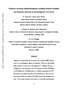
Fig. 2 shows classical and renormalized spectra for S = 12 in two representative fields. At H = 0, the only nonvanishing correction Σ(3) (k) yields a 16% enhancement of magnon energies in the entire Brillouin zone [5,7]. In low fields the magnon spectrum resembles zero-field result except the vicinity of the BZ center. The mode at k = 0 describes a uniform precession of spins about H and, for axially symmetric systems its classical frequency ω0 = H is exact, i.e., not changed by quantum effects [12]. With increasing field the cubic terms grow and push down magnon energies. Above 0.7Hc , correction from Σ(1) (k, ωk ) exceeds 50% of ωk signifying a break down of the 1/S perturbation expansion for spin-wave frequencies (9). The correct renormalized spectrum plotted in Fig. 2 is recovered by solving the Dyson equation

(2)

(b)

FIG. 1. Lowest-order diagrams contributing to the magnon self-energy.

There are two interaction terms with cubic vertices ˆ (3) [10] from H 1 Vˆ1 = 2! 1 Vˆ2 = 3!

X

1−2−3=Q


(1) Γ1;23 b†3 b†2 b1 + h. c. ,

X


(2) Γ123 b†3 b†2 b†1 + h. c. ,

1+2+3=Q

(6)

ω − ωk − Σ(k, ω) = 0.

where we abbreviated momenta with their subscripts. The first term Vˆ1 is responsible for the hybridization between single- and two-magnon spectra and is the principal interaction of the problem. The vertices are given by √ (1) Γ1;23 = − 8S sin2θΦ(k; q),

Standard 1/S expansion breaks down for any finite S when the bottom of two-magnon continuum becomes nearly degenerate with a part of the single-magnon spectrum for H close to the decay threshold field H ∗ . Unrenormalized “classical” value of H ∗ is calculated by ex˜ The cubic panding Eq. (5) up to the third order in k. factor α is anisotropic and vanishes first for k˜x = k˜y at H ∗ = √27 Hc ≈ 0.756Hc. At H > H ∗ the magnon self-energy acquires imaginary part due to spontaneous two-magnon decays, which obey the energy conservation law

Φ(1; 23) = γ1 (u1 + v1 )(u2 v3 + v2 u3 ) + γ2 (u2 + v2 )(u1 u3 + v1 v3 ) + γ3 (u3 + v3 )(u1 u2 + v1 v2 ), (7) √ (2) and Γ123 = − 8S sin2θF (k, q), where similar expression for F (k, q) can be found in [10]. The lowest-order contributions to the self-energy shown in Fig. 1 are Σ

(1)

2

(k, ω) = 4S sin 2θ

X q

Σ(2) (k, ω) = −4S sin2 2θ

ωk = ωq + ωk−q+Q .

Φ(k; q)2 , (8a) ω − ωq − ωk−q+Q + i0

X q

F (k, q)2 . ω +ωq +ωQ−k−q −i0

(10)

(11)

Spin-wave is stable, if Eq. (11) has only trivial solutions: q = k, Q. In Pthis case, the two-magnon density of states ρ2 (k, ω) = q δ(ω − ωq − ωk−q+Q ) vanishes at ω < ωk . ρ2 (k, ω) has Van Hove singularities determined by symmetry extrema k − q∗ + Q = q∗ + G, where G is a reciprocal lattice vector. At H > H ∗ , one of these points q∗ = (k + Q)/2 crosses the one-magnon state if

(8b)

The first term describes a virtual decay of a magnon into two-particle intermediate states. Frequency-independent 2

ωk ≥ 2ω(k+Q)/2 .

In the limit k˜ → 0 the decaying rate is small and can be found analytically. The self-consistent Born approximation (SCBA) with dressed lines in Fig. 1a gives

(12)

When applied to the phonon mode, Eq. (12) is equivalent to the previously used condition α > 0 [note the difference between k and k˜ in Eqs. (1) and (12)]. At H > H ∗ , classical magnons (5) decay in the region around k = Q and remain stable in the vicinity of uniformly precessing mode k = 0 with the decay threshold boundary given by equality sign in Eq. (12).

Im Σ(1) (k, ω) = −4πS sin2 2θ Z d2 q 2 Φ (k; q)φ(ω − ωq − ωk−q+Q ), (14) × (2π)2 R where function φ(ω) is normalized by φ(ω)dω = 1 and has a characteristic width of the order of a sum of decay rates of created magnons. √ Using the asymptotic form Φ(k; q) ≈ − 43 [k˜q˜(k˜ − q˜)/ 2 cos3 θ]1/2 we find

3

H=0.75HC

˜ + αk˜2 − iβ k˜2 ), ωk ≈ ck(1 (15) √ with β = (9 sin2 θ/64π 2 cos3 θ)2/3 . Similar to a 3D case [8], this expression for β is valid beyond a narrow field region near H ∗ determined by higher-order nonlinearities. Another region in BZ, where damping is small and excitations are well defined, lies near the zone center. This follows from the same arguments [12], which predict no effect on ω0 from quantum fluctuations, since the exact frequency at k = 0 is real and has no imaginary part. The spin-wave damping in the entire BZ is considered by using the magnon spectral function A(k, ω) = − π1 ImG(k, ω), where G(k, ω) is calculated in the Born approximation. Results for A(k, ω) at H = 0.85Hc and H = 0.9Hc are presented in Fig. 3(a) and 3(b), respectively. In the non-self-consistent approximation (dashed lines), A(k, ω) consists of a narrow one-magnon peak and two-magnon side-band, which exhibits loose maximum at higher energies. The quasiparticle peaks survive even in the classical decay region Eq. (12), because hybridization pushes them out from the two-magnon continuum. This spurious feature arises due to the lack of self-consistency, as the two sides of Eq. (11) are treated with different accuracy in the non-SCBA. That is, the magnon energy is renormalized while the energy of the continuum (righthand side) is given by a classical expression. Peaks disappear in the SCBA, which takes into account modification of two-particle continuum due to renormalization of onemagnon states. We performed numerical solution of the Dyson equation in the SCBA with 96×96 k-points in BZ. Results are plotted in Fig. 3 by solid lines. Our analysis shows that a self-supporting instability intensifies at H = 0.85Hc for magnons from the region k < Q/2, which are classically stable but become strongly damped since they lie in the decay region for renormalized spectrum. Magnons peaks in A(k, ω) are strongly suppressed (H = 0.85Hc) and disappear (H = 0.9Hc ) because of the shift of single-particle pole in G(k, ω) from the real axis into the complex plane due to rapidly growing decay surface (11). This is in contrast with Pitaevskii’s scenario for superfluid 4 He, where the pole’s residue becomes vanishingly small [8]. Single-magnon excitations reappear again only at H ≈ 0.99Hc, where the decaying vertex Γ(1) (1; 23) is small.

ω(κ)

2

1

H=0.1HC 0

0.0

0.2

0.4

η

0.6

0.8

1.0

FIG. 2. Magnon dispersion for k = π(η, η): (i) thin dashed lines represent the classical spectrum ωk ; (ii) dot-dashed lines are ωkpert ; (iii) solid lines are solution of the Dyson equation. For H = 0.1Hc , curves (ii) and (iii) are indistinguishable.

Pitaevskii argued that such boundaries are actually termination points of the spectrum [8]. This fact is a consequence of logarithmic divergence of the one-loop diagram near the threshold: Σ(1) (k, ω) ∝ ln(−∆˜ ω /R), where ω ˜ = ∆ω + vc ∆k, vc is a velocity of created magnons, and R is a cut-off. Termination point for the decay threshold into a pair of rotons is known in the spectrum of superfluid 4 He. Since the self-energy is singular, a proper renormalization of the cubic vertex is necessary in that case [8]. Our problem, however, is different, because two new magnons created in an elementary decay process are again unstable. Near the decay threshold, the dominant contribution to Σ(1) arises from the close vicinity of q = (k + Q)/2, therefore we can approximate Im ωq ≈ Im ωk−q+Q = 12 Γ. Even small Γ’s remove completely divergence of the diagram (Fig. 1a): h √∆˜ π ∆˜ ω i ω 2 +Γ2 (1) . (13) Σ (k, ω) ∝ ln − i +arctan R 2 Γ This analysis leads us to two conclusions: (i) vertex corrections can be neglected, but instead a self-consistent treatment of intermediate magnons and their decaying rates is required; (ii) the boundary (12) between stable and decay regions in BZ is smeared and at H > H ∗ all magnons simultaneously acquire finite life-times. 3

×

50

0

X (uq vk−q+Q +vq uk−q+Q )2 δ(ω −ωq −ωk−q+Q ), q

yy

S (k, ω) = πS(uk − vk )2 A(k, ω),

H=0.85HC 1/6

(16)

S zz (k, ω) = πS cos2 θ(uk−Q +vk−Q )2A(k − Q, ω) X +π sin2 θ (uq vk−q +vq uk−q )2 δ(ω −ωq −ωk−q ),

40

1/3

q

1/2

Α(κ,ω)

30

where we use the unperturbed spectrum for the twomagnon contributions. These two-magnon contributions described by the last terms in S xx and S zz are negligible in high fields because of small factors vk ∼ cos2 θ. In the same approximation uk ≈ 1 except for close vicinity of Q. Thus, in high fields H ∗ < H < Hc the longitudinal component S zz (k, ω) reduces to its elastic part, whereas transverse components S xx (k, ω) and S yy (k, ω) are proportional to A(k, ω) with approximately same momentum independent prefactors. In conclusion, the nonlinear coupling between one- and two-magnon states, which exists only in the canted AFM phase, becomes very important in high fields. Together with the field-induced kinematic instability of the spectrum this interaction leads to suppression and disappearance of single-magnon excitations for H ∗ < H < Hc . Therefore, an intriguing situation arises in the high field regime: the ground state of an ordered quantum AFM is nearly classical, while the excitation spectrum and the dynamical response are strikingly different from the classical results. Though, our analysis was restricted mainly to the spin- 12 AFM in 2D, the qualitative picture remains valid for other values of S and for 3D. We are grateful to D. I. Golosov, T. Nikuni, and V. I. Rupasov for useful discussions. The work of A.L.C. was supported by the NSERC of Canada.

2/3 20

5/6 10

0

0

1

2

3

ω

50

4

0

H=0.9HC 1/6

40

30

Α(κ,ω)

1/3 1/2 2/3

20

5/6 10

0

0

1

2

ω

3

4

FIG. 3. Magnon spectral function for several points k = π(η, η), (a) H = 0.85Hc , (b) H = 0.9Hc . Thin dashed lines represent the non-SCBA. Solid lines are the results of the SCBA. Corresponding values of η are shown near each curve.

∗

[1] [2] [3] [4]

To complete our study, we investigate now the highfield dynamical response of the square-lattice AFM, which is probed in neutron diffraction experiments. Our calculation of the dynamical structure factor S αβ (k, ω) = R β dthSkα (t)S−k ieiωt is standard. We express it at T = 0 via the spin Green’s function Gαβ (k, t) = β −ihT Skα (t)S−k i by S αβ (k, ω) = −2θ(ω)Gαβ (k, ω). The latter is related to the boson Green’s function by using Eq. (3) and the Dyson-Maleev transformation. The result for the inelastic part of the dynamical structure factor is

[5] [6] [7] [8] [9] [10] [11] [12]

S xx (k, ω) = πS sin2 θ(uk +vk )2A(k, ω) + π cos2 θ 4

On leave from the Institute of Semiconductor Physics, Novosibirsk, 630090, Russia. D. C. Dender et al ., Phys. Rev. Lett. 79, 1750 (1997). G. Chaboussant et al ., Phys. Rev. B 55, 3046 (1997). P. R. Hammer et al ., J. Appl. Phys. 81, 4615 (1997). K. Osano, H. Shiba, and Y. Endoh, Prog. Theor. Phys. 67, 995 (1982). T. Oguchi, Phys. Rev. 117, 117 (1960). A. B. Harris et al ., Phys. Rev. B 3, 961 (1971). C. M. Canali, S. M. Girvin, and M. Wallin, Phys. Rev. B 45, 10131 (1992). E. M. Lifshits and L. P. Pitaevskii, Statistical Physics II (Pergamon, Oxford, 1980). E. Manousakis, Rev. Mod. Phys. 63, 1 (1991). M. E. Zhitomirsky and T. Nikuni, Phys. Rev. B 57, 5013 (1998). the Holstein-Primakoff transformation used in Ref. [10] yields identical results to a given order. D. I. Golosov and A. V. Chubukov, Sov. Phys. Solid State 30, 893 (1988).