Interactive Continuous Collision Detection for Non ... - CiteSeerX

The Visual Computer manuscript No. (will be inserted by the editor)

Xinyu Zhang · Minkyoung Lee · Young J. Kim+

Interactive Continuous Collision Detection for Non-Convex Polyhedra http://graphics.ewha.ac.kr/FAST

Abstract We present a highly interactive, continuous collision detection algorithm for rigid, general polyhedra. Given initial and final configurations of a moving polyhedral model, our algorithm creates a continuous motion with constant translational and angular velocities, thereby interpolating the initial and final configurations of the model. Then, our algorithm reports whether the model under the interpolated motion collides with other rigid polyhedral models in environments, and if it does, the algorithm reports its first time of contact (TOC) with the environment as well as its associated contact features at TOC. Our algorithm is a generalization of conservative advancement [20] to general polyhedra. In this approach, we calculate the motion bound of a moving polyhedral model and estimate the TOC based on this bound, and advance the model by the current TOC estimate. We iterate this process until the inter-distance between the moving model and the other objects in the environments becomes below a user-defined distance threshold. We pose the problem of calculating the motion bound as a linear programming problem and provide an efficient, novel solution based on the simplex method. Moreover, we also provide a hierarchical advancement technique based on bounding volume traversal tree to generalize the conservative advancement for non-convex models. Our algorithm is relatively simple to implement and has very small computational overhead of merely performing discrete collision detection multiple times. We extensively benchmarked our algorithm in different scenarios, and in comparison to other known continuous collision detection algorithm, the performance improvement ranges by a factor of 1.4 ∼ 45.5 depending on benchmarking scenarios. Moreover, our algorithm can perform CCD at 120 ∼ 15460 frames per second on a 3.6 GHz Pentium 4 PC for complex models consisting of 10K ∼ 70K triangles. Department of Computer Science and Engineering Ewha Womans University, Seoul, Korea E-mail:{zhangxy|minkyounglee|kimy}@ewha.ac.kr Tel.: +82-2-3277-4068 Fax: +82-2-3277-2306 + : Corresponding Author

Keywords Continuous Collision Detection, Convex Decomposition, Conservative Advancement, Dynamics Simulation

1 Introduction Collision detection (CD) is a problem of testing possible interference between geometric models in space. Many graphics applications require fast and reliable CD to simulate the physical presence of objects in virtual space. These cover a wide range of applications such as physically based animation, virtual environments, virtual characters, geometric modelling, etc. As a result, CD has been extensively studied in the literature and many efficient CD algorithms are known. At a broad level, depending on how CD algorithms handle the motion of objects, they can be categorized into two types, discrete CD and continuous CD. Discrete CD algorithms check for interferences between static objects. When objects are moving, discrete CD algorithms are often called at fixed time intervals to deal with the motion of objects. However, it is well known that when objects are moving at a high speed or objects are thin, discrete CD algorithm can easily miss a collision between sampled time instances [24]. Meanwhile, continuous CD (CCD) algorithms take the object’s continuous motion into account and accurately report the first time of contact (TOC) between moving objects if there occurs a collision. Recently, CCD has drawn much attention from different communities because of the need for correctly dealing with dynamic nature in applications. The major strength of using CCD in dynamic applications lies in a fact that the result of CCD always guarantees nonpenetration between moving objects. For example, in rigid body dynamics, finding an accurate TOC between simulated bodies is crucial to enforce non-penetration constraints in the simulation [3, 25], and CCD is directly applicable to finding a TOC. In 6DOF haptic rendering, a recent technique based on CCD enables God-object type haptic rendering for object/object interactions thanks to the non-penetration condition imposed by CCD [22]. In sampling-based robot mo-

2

tion planning such as probabilistic roadmap method (PRM), it is crucial to find a continuous, collision free path between two configurations of a moving robot, and CCD plays an important role in finding one [28]. However, the major limitation in existing CCD algorithms is that they are, in general, much slower than discrete CD algorithms. This often limits the applicability of CCD algorithms to many potential applications.

Xinyu Zhang et al.

the preliminary concepts to understand our algorithm and provide an overview of our algorithm. In Sec. 4, we explain how we efficiently calculate the bound of motion and generalize conservative advancement to general polyhedra in Sec. 5. In Sec. 6, we show the performance results of our algorithm in different benchmarking scenarios and conclude the paper in Sec. 7. 2 Previous Work

1.1 Main Results In this paper, we present a fast method to perform CCD between moving, general polyhedra. Our algorithm outperforms known CCD methods by utilizing the connectivity information residing in polyhedra and exploiting the coherence in the continuous motion. Given initial and final configurations of a moving polyhedral model, our algorithm creates a continuous motion with constant translational and angular velocities, there interpolating the initial and final configurations of the model. Then, our algorithm reports whether the model under the interpolated motion collides with other rigid polyhedral models in environments, and if it does, the algorithm reports its first time of contact (TOC) with the environment as well as its associated contact features at TOC. The main ingredient of our algorithm is a generalization of conservative advancement [20] to general polyhedra. In this approach, we calculate the motion bound of a moving polyhedral model and estimate the possible TOC based on this bound and the inter-distance between the model and other objects in the environment, and advance the model by the current TOC estimate. We iterate this process until the inter-distance becomes less than a user-defined distance threshold. We pose the problem of calculating the motion bound as a linear programming problem and provide a novel, efficient solution based on the simplex method. Moreover, we also provide a novel, hierarchical advancement technique based on bounding volume traversal tree to generalize conservative advancement for non-convex models. Our algorithm is relatively simple to implement in the sense that one needs to make only minor modifications to existing discrete CD library to implement our algorithm. As a result, our algorithm has very small computational overhead of iterating discrete CD multiple times. We extensively benchmarked our algorithm in different scenarios, and in comparison to other known continuous collision detection algorithm, the performance improvement ranges by a factor of 1.4 ∼ 45.5 depending on benchmarking scenarios. Moreover, our algorithm can perform CCD at 120 ∼ 15460 frames per second on a 3.6 GHz Pentium 4 PC for complex models consisting of 10K ∼ 70K triangles.

1.2 Organization The rest of this paper is organized as follows. In Sec. 2, we briefly survey work relevant to ours. In Sec. 3, we explain

In this section, we give a brief survey of the earlier work related to continuous collision detection and distance calculation. 2.1 Discrete Collision Detection and Distance Calculation Most of the prior work on collision detection has focused on discrete CD algorithms. We refer the readers to see [18] for an excellent survey on the field. These include specialized algorithms for convex polytopes that exploit motion coherence between successive time steps, general algorithms for polygonal or spline models that pre-compute a spatial partitioning or bounding volume hierarchies (BVH). Calculating Euclidean distance between polygonal models has been extensively studied in the literature. For convex polytopes, an efficient theoretical algorithm [8], linear programming-based approach [29], Minkowski-sum and convex optimization approach [11], Voronoi marching exploiting motion coherence [19] and multi-resolution approach [9, 13] have been proposed. For non-convex models, typically BVH has been employed to deal with the non-convexity in the models. A convex hull tree-based scheme combined with Voronoi marching has been introduced and shown to work at highly interactive rates for complex polyhedral models [10]. A hybrid BVH scheme using different types of swept sphere volumes has been presented to calculate distance between generic polygonal models [17]. 2.2 Continuous Collision Detection A few algorithms have been proposed for CCD. More specifically, there are five different approaches presented in the literature: algebraic equation solving approach [6, 7, 14, 23], swept volume approach [1], adaptive bisection approach [24, 28], kinetic data structures (KDS) approach [2, 15, 16], and Minkowski sum-based approach [5]. However, most of these approaches do not work in real-time or work for only simple or convex models. Only the adaptive bisection approach has shown interactive performance for relatively complex polygonal models; however, it is designed to handle models in polygon soups and does not take advantage of connectivity information residing in polyhedral models and motion coherence in CCD computations. Recently, CCD for articulated models have been proposed [26, 27]. [26] is applicable to simple, capsule-shaped


avatar models in VR environments and shows interactive performance, whereas [27] works for articulated models but shows only near real-time performance.

3 Overview We start this section by introducing the notations and definitions used throughout this paper. Then, we will briefly explain the basic idea of conservative advancement (CA) and distance calculation methods that our CCD algorithm is based on. Based on these concepts, we provide an overview of our algorithm later. 3.1 Notations and Definitions We use a bold symbol to differentiate a vector quantity from a scalar value (e.g., the origin, o). Let A and B be two polyhedron. Without loss of generality, we assume that A is a moving object under rigid transformation M and B is fixed in space since we can find relative rigid transformation with respect to each other. Further, we assume that the initial and final configurations of A are given as q0 and q1 at its corresponding time, t = 0 and t = 1, respectively. We use A (t) as a placement of A under rigid transformation M at time t; i.e., A (t) = M(t)A . Then, the problem of CCD can be formulated as checking whether Eq. 1 is non-empty: { t ∈ [0, 1] | A (t) ∩ B 6= 0}. /

(1)

Furthermore, if Eq. 1 is non-empty, we want to compute the minimum value of t that satisfies this equation, known as the time of contact, tT OC . 3.2 Conservative Advancement for Convex Polytopes

p v + w A

n d

B

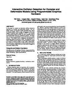
Fig. 1 Conservative Advancement.

The CA is a simple technique that computes an upper bound of tT OC by repeatedly advancing A by ∆t toward B while avoiding collision [20,21]. Here, ∆t is calculated based on the closest distance d(A (t), B) between A (t) and B, and the upper bound µ of the motion along d(A (t), B) traced by A (t) per unit second. More specifically, in Fig. 1, let p be a point on A , and let n be the closest direction vector that realizes d(A (t), B). Moreover, let µ be an upper bound of the distance along d(A (t), B) travelled by any p

3

on A per second. Then, A can advance from time t to time t + ∆t without collision: µ∆t ≤ d(A (t), B) d(A(t), B) ∆t ≤ µ

(2)

The proof is simple, and we refer the readers to see [21] for detail. In Eq.2, the smaller value of µ or the larger value of d(A (t), B), the larger CA step size ∆t we can have. Thus, we need a tight upper bound of motion µ and tight lower bound of distance d(A (t), B). Notice, however, that the technique presented in [21] works only for convex objects. Later in Sec. 5, we will provide novel techniques to generalize CA to non-convex objects and also provide a tighter upper bound of µ by considering both the linear and rotational motions in Sec. 4.

3.3 Distance Calculation using Convex Decomposition It is easier to calculate the distance between convex polytopes than computing it for general, non-convex polyhedra. In particular, Voronoi Marching [9, 19] exploits motion coherence involved in distance calculation and is a good choice for CA as CA requires repeated calculations of distance and thus the motion coherence is high between successive computations. For distance calculation between general polyhedra, a BVH-based technique using convex hull tree is known to work well [10]. As preprocess, the algorithm decomposes a given, general polyhedron A into convex pieces cA i and recursively builds a convex hull tree where each node in the tree corresponds to a convex hull of its children nodes. Note that the convex decomposition scheme employed in [10] is merely surface decomposition in which the union of cA i covers only the boundary of A , and this is sufficient for distance calculation. At run-time, starting from the root nodes of two convex hull trees, the algorithm simultaneously traverses the two trees while performing Voronoi marching on the tree nodes and calculating their distance as well as their associated closest features. The recursive traversal continues until the closest distance cannot be further reduced. This tree traversal process can be also thought of as implicitly building a bounding volume traversal tree (BVTT) between two convex hull trees. The concept of BVTT will be explained in more detail in Sec. 5.1.

3.4 Our Approach In our algorithm, we assume that two non-convex polyhedra A and B are given and only the initial and final configurations of A are known as q0 , q1 . As in many applications, since the actual governing motion of A is unknown [24], we use an arbitrary in-between motion that interpolates q0 , q1 .

4

Xinyu Zhang et al.

As a result, we can express a continuous motion M(t) in terms of time that governs the motion of A . In order to find tT OC between non-convex polyhedra A and B, a naive approach based on convex decomposition and CA can be devised as in Alg. 1. Algorithm 1 Naive CCD using Convex Decomposition Input: A moving polyhedron A and its initial and final configurations q0 , q1 , a fixed polyhedron B. Output: Calculate tT OC . B 1: As preprocess, decompose A and B into convex pieces, cA i ,cj , as in [10]. 2: Compute an interpolating motion M(t) from q0 , q1 . 3: repeat B 4: for each pair of convex pieces (cA i , c j ) do B 5: Calculate their distance d(cA i , c j ) using [9] and find their closest direction vector n. 6: Calculate the motion bound µ of cA i using n. d(cA ,cB )

7: Calculate ∆ti, j = i µ j based on Eq. 2. 8: end for 9: Find ∆t := min(∆ti, j ). 10: Advance A (t) by ∆t. 11: until d(A (t), B) becomes less than a user-provided threshold 12: return tT OC

There are two severe problems in Alg. 1, however. First of all, if the numbers of convex pieces in A , B are ηA , ηB , each CA step (step 4) requires O(ηA ηB ) time. Additionally, the motion bound µ (step 6) can become overly conservative and many CA steps (step 11) would be required. These two problems can result in poor performance of the naive algorithm. To address the first issue, instead of calculating the distance between decomposed convex pieces of A , B, we calculate the distance between A , B themselves using the technique presented in Sec. 3.3 and remember the nodes in convex hull trees that realize this distance, called front nodes. The union of these nodes is a super set of the union of convex pieces thanks to the convex hull property of convex hull tree. Notice that the distance between the front nodes has been already calculated during the BVH traversal scheme in Sec. 3.3. We perform CA only to these front nodes (Sec. 5). Moreover, to efficiently calculate µ between these front nodes, we take the closest vector direction n between the nodes and project its translational and rotational motion onto n (Sec. 4). Overall, our algorithm works as in Alg. 2.

Algorithm 2 CCD using Hierarchical Advancement Input: A , B and q0 , q1 Output: Calculate tT OC . 1: As preprocess, decompose A and B into convex pieces and construct their convex hull trees, CHTA ,CHTB . 2: Compute an interpolating motion M(t) from q0 , q1 . 3: repeat 4: Calculate d(A (t), B) between A (t) and B using B CHTA ,CHTB and remember the pairs of front nodes hA i ,hj in the trees that were traversed to calculate d(A (t), B). During B the traversal, d(hA i , h j ) and closest direction vector n(i, j) are stored {Alg. 3 in Sec. 5}. B 5: for each pair of (hA i , h j ) do B 6: Retrieve already calculated d(hA i , h j ) and n(i, j). 7: Calculate the motion bound µ(i, j) by projecting both the translational and rotation motion of hA i onto n(i, j). d(hA ,hB )

i j 8: Calculate ∆ti, j = µ(i, j) . 9: end for 10: Find ∆t := min(∆ti, j ). 11: Advance A (t) by ∆t. 12: until d(A (t), B) becomes less than a user-provided threshold 13: return tT OC

4.1 Motion Interpolation In many applications involving motion such as physically based animation, rapid prototyping, virtual environments and robot motion planning, its governing motion is often either unknown or cannot be represented as a closed form. This is because the motion employed in these application is controlled interactively by a user [24], or purely random [28], or should be calculated numerically [4]. Therefore, in our CCD algorithm, we only assume that the initial and final configurations of A are known (q0 , q1 ), and need to find a continuous, rigid motion M that interpolates q0 , q1 . We further assume that q0 is collision-free; otherwise, we trivially report that tT OC is zero by performing discrete CD at q0 . Different types of interpolation motions have been used in other CCD algorithms: screwing motion [14, 24], ballistic motion [21] and linear motion in configuration space [28, 5]. In our case, we choose the linear motion with constant translational and angular velocities because of its simplicity. In fact, some application such as robot motion planning requires linear motion in configuration space [28]. Let us represent the configurations q0 , q1 as their translational (T) and rotational components (R): q0 = (R0 , T0 ), q1 = (R1 , T1 ). We want to represent the interpolating motion M(t) at time t as:

4 Motion Bound Calculation

M(t) =

Since our algorithm does not assume a closed form of the continuous motion of a moving object, we first explain how we model the continuous motion when only its initial and final configurations are given, and also show how we can efficiently calculate the motion bound µ of a moving object under such a motion.

R(t) T(t) (0, 0, 0) 1

Then, T(t) = T0 + tv R(t) = cos (ωt).A + sin (ωt).B + C

(3)


Here, v = T1 − T0 is the constant translational velocity of the center of mass (COM) of A . Furthermore, A = R0 − uuT .R0 B = u∗ .R0 C = uuT .R0

5

and ri exists only on the surface of a convex polytope, maximizing |c · ri | becomes a linear programming problem. As a result, we have: µ = max |c1 · ri | + c2 i

(5)

subject to ri · nk ≤ dk , k = 1 . . . |A |

Here, (u, ω) is the constant angular velocity of A , extracted where c1 = n×ω, c2 = |v·n|, and |A | is the number of faces ∗ in a convex polytope A , and x · nk = dk is the plane equation from R1 R−1 0 and u is the skew symmetric matrix; i.e., if for the kth face in A . x y z T u = (u , u , u ) , then There are many known methods to efficiently solve the   z y linear programming in Eq. 5 [29]. In particular, the simplex 0 −u u ∗ z x method or the hill climbing method works well in this simple   u 0 −u u = case. The main idea is, given a query direction c1 , we want to −uy ux 0 find a vector ri on the surface of a convex polytope A whose direction is closest to the direction of c1 . This type of query is also known as support mapping of c1 [30] or extremal ver4.2 Motion Projection tex query along c1 [9]. A simple method that works well in Given the interpolating motion, M(t), now we explain a novel practice is the use of a lookup table as presented in [9]. In technique of how we can calculate the tight upper bound µ this approach, we sample the possible directions of c1 , and of motion. For now, we assume that both the moving A and precalculate its extremal vertex ri , and store their associafixed objects B are convex, and the motion bound calculations in a lookup table. At run-time, given c1 , we look up the tion technique explained here will be applied to non-convex closest vector cˆ to c1 in the table and use its associated exobjects in Sec. 5 by decomposing A , B into convex objects, tremal vertex as a starting point in the hill climbing to further calculating the motion bound for each convex pair, and tak- maximize Eq. 5. ing its minimum. Let pi be a point on A , and as A undergoes M, pi will trace out a trajectory pi (t) in 3D Euclidean space. Consider 5 Hierarchical Advancement its velocity p˙ i (t) = v + ω × ri (t), where v, ω are the linear velocity of the center of mass (COM) and angular velocity By plugging µ in Eq.5 into the step (6) in the naive CCD of A , respectively, and ri = pi − RCOM where RCOM is the algorithm, Alg. 1, we can devise a CCD algorithm for nonposition of the COM. Notice that v, ω are constant between convex polyhedra and accelerate its performance considerthe time interval of [0, 1] in our case. Then, the undirected ably. However, due to the quadratic complexity of O(ηA ηB ) in Alg. 1, the algorithm does not scale well to complicated motion bound µu of A can be expressed as: non-convex models. Z 1 In this section, we present a novel, efficient scheme based (4) ||p˙ i (t)|| dt µu = max on the concept of bounding volume traversal tree (BVTT) i 0 that can handle the quadratic complexity in Alg. 1. Now µu can be an upper bound of motion that Eq. 2 uses, but we relax the convexity restrictions of A , B and assume that we get a tighter upper bound µ by projecting pi (t) onto n, they are non-convex polyhedra. which is the closest direction vector between A and B: Z 1

max i

≤ max i

Z0

|p˙ i (t) · n| dt

|v · n + ω × ri · n| dt

≤ |v · n| + max

Z

i

≤ |v · n| +

Z

|ω × ri · n| dt

max(|ω × ri · n|) dt i

≤ |v · n| + max(|ω × ri · n|) i,t

=µ Since v, n, ω are constants during the time interval of ∆t, calculating µ boils down to maximizing |ω × ri · n|. Further, it is equivalent to maximizing |(n × ω) · ri | since (ω × ri ) · n = (n × ω) · ri . Moreover, because n × ω = c1 is a constant

5.1 Bounding Volume Traversal Tree As preprocess, our algorithm decomposes each of the given non-convex polyhedra into convex pieces, and recursively builds a bounding volume hierarchy (BVH) where each BV node corresponds to the convex hull of its children nodes (i.e., convex hull tree), as explained in Sec. 3.3. Given two BVHs (CHTA ,CHTB ) of A , B, when we calculate the distance between A , B at given time t, starting from the root nodes of CHTA ,CHTB , pairwise distance B calculation between the nodes hA i , h j in CHTA ,CHTB is recursively performed based on Voronoi marching. Each reB cursion step requires distance calculation d(hA i , h j ) between B A B some pair of nodes hA i , h j in CHTA ,CHTB , and d(hi , h j ) is compared to the global minimum d of previously calcuB A B lated d(hA k , hl )’s during the recursion. If d(hi , h j ) < d,

6

Xinyu Zhang et al.

B the recursive traversal for hA i , h j continues; otherwise, it stops.

Based on the BVTT, we can devise an efficient hierarchical algorithm to perform CA between non-convex polyhedra A , B. The main idea of this method is based on the following observations:

Front

CHTA

CHTB

5.2 Conservative Advancement for General Polyhedra

BVTT

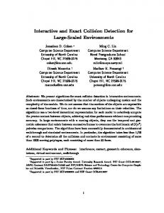
Fig. 2 Bounding Volume Traversal Tree. Two BVHs and their BVTT during distance query. Only solid-colored nodes are actually generated in BVTT.

The bounding volume traversal tree (BVTT) is a special recursion tree generated during the distance query, as illustrated in Fig. 2. BVTT was originally introduced by [17] to measure the cost of a BVH traversal scheme. In our case, each node h(i, j) in a BVTT corresponds to a pair of convex B A B hull nodes hA i , h j . Furthermore, d(hi , h j ) and the closB est direction vector n(i, j) that realizes d(hA i , h j ) are also stored at h(i, j). The front in a BVTT refers to a collection of the leaf nodes in the tree, generated during the distance query at run-time. In practice, the size of front is much smaller than the size of all possible combinations between convex pieces in A , B. We take advantage of this fact to reduce the quadratic complexity in Alg. 1. Algorithms for distance calculation between non-convex polyhedra as well as building its corresponding BVTT are explained in Alg. 3.

Algorithm 3 BVTT Input: BVH nodes hi , h j , Current distance dCurrent Output: Return the closest distance d(hi , h j ) 1: {Initially, BVTT(CHTA .root, CHTB .root, ∞) is called. } 2: {A BVTT node h(i, j) is created.} 3: Perform Voronoi marching on hi , h j to find d(hi , h j ) and its closest vector n(i, j). 4: if d(hi , h j ) < dCurrent then 5: if h j is not a leaf node in CHTB then 6: d1 = BVTT(hi , h j .LeftChildTree). 7: d2 = BVTT(hi , h j .RightChildTree). 8: return min (d1 , d2 ). 9: else if hi is not a leaf node in CHTA then 10: d1 = BVTT(hi .LeftChildTree, h j ). 11: d2 = BVTT(hi .RightChildTree, h j ). 12: return min (d1 , d2 ). 13: else 14: {Mark h(i, j) as front and n(i, j) is stored at it.} 15: return d(hi , h j ) 16: end if 17: else 18: {Mark h(i, j) as front and n(i, j) is also stored at it.} 19: return d 20: end if

1. The union of the front nodes h(i, j) in BVTT is a superset of the union of all the pairwise combinations of convex B pieces (cA i , c j ) in A , B. 2. The front nodes h(i, j)’s are the nodes that are discovered during closest distance query, so that these nodes have a higher probability than other convex nodes in BVTT to be collided at tT OC or to be reused for successive distance query at next CA step. The observation (1) guarantees that our algorithm based on performing CA on the front is conservative. Thanks to the observation (2), our algorithm is not overly conservative and as experimentally shown in Sec. 6, it is quite efficient in practice (i.e., few CA iterations). In fact, the observation (2) has been similarly used in discrete distance query when high motion coherence exists. In other words, the witness convex pieces that realize closest distance at time step t tend to be a witnesses again for the next time step t + ∆t when the underlying motion has high coherence [10]. In our case, since our algorithm requires successive invocation of CA steps, it has a similar effect of having high motion coherence and thus the observation (2) is sound. Based on the aforementioned observations, our algorithm applies an atomic, convex CA operation to each node h(i, j) in the front, estimates its individual time of contact ∆tT OC (i, j), and takes its minimum as ∆tT OC . Then, we advance A by ∆tT OC and iterate another CA step until d(A (t), B) becomes smaller than a user-provided distance threshold. Finally, at tT OC , we perform one-time discrete distance query to find all the relevant contact features such as face/vertex and edge/edge. This algorithm has been summarized earlier in Alg. 2. The major strength of our hierarchical CA algorithm can be also summarized as follows: B – The main bottleneck in Alg. 2 is the computation of d(hA i ,hj ) and n(i, j). However, these are already calculated as part of distance calculation between A and B, as presented in Alg. 3. As a result, the hierarchical CA has very little overhead over discrete distance calculation d(A (t), B) at time t. – Typically, since the size of the front nodes is small, the step (5) in Alg. 2 has a much lower number of iterations compared to O(ηA ηB ).

6 Results and Discussions Now we present our implementation results and discuss its performance.


7

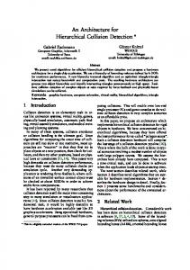
Fig. 3 Benchmarking Models. From left to right, bunny (70K tri.), Santa (37K tri.), torus-knots (2.8K, 11K, 34K tris.), a ring (10K tri.).

6.1 Implementation Results We have implemented our CCD algorithm using C++ on Windows XP, equipped with Intel P4 3.6GHz CPU and 2GB main memory. We have used a public-domain proximity library, SWIFT++1 for distance calculation and convex decomposition for non-convex polyhedra, and have modified it to serve our purpose. We also take advantage of the extremal vertex query function provided in SWIFT++ to implement Eq. 5. Thus, in some sense, our implementation can be considered as a continuous version of SWIFT++.

6.2 Benchmarking

4. Rigid Body Dynamics for Bunnies (Fig. 8-Left): Using HAVOKTM2 , we perform rigid body dynamics to simulate the falling of a red bunny against a blue one, each consisting of 26K triangles, due to gravity. Each simulation step provides q0 , q1 of the blue moving bunny, plug these into our CCD algorithm, and measure the performance. Moreover, in order to create artificial interpenetration at q1 from this simulation (the simulation itself is collision-free all the time), we slightly modify the q1 before impact, and thus we can ask our CCD algorithm to find tT OC . 5. Rigid Body Dynamics for Rings (Fig. 8-Right): We conduct similar dynamics experiments for a ring consisting of 10K triangles.

The resulting performance of our algorithm, named as In order to measure the performance of our algorithm, we 3 employ different benchmarking models in various complex- FAST , for the above benchmarks is shown in Fig.’s 4, 5, 7 ities (ranging from 10K to 70K triangles) as shown in Fig. and 8: it includes timings (in milli-seconds) and the num3. These models are highly non-convex, and we use them in ber of CA iterations of our algorithm (FAST). We also meadifferent benchmarking scenarios as below. The user-controlled sure the performance of a known CCD method, CONTACT threshold of distance to find tT OC is 0.001 throughout all the [24], for each benchmarking scenario and compare it with ours. CONTACT can be thought of as a continuous version experiments. of the OBB algorithm [12] and uses a screwing formula1. Santa vs Thin Board (Fig. 4): Given two configurations tion for motion interpolation. As a result, our algorithm and of q0 , q1 of a highly non-convex Santa model with 37888 CONTACT do not perform the exactly same CCD operatriangles, separated by approximately 5 times the bound- tion but both of the algorithms are able to calculate tT OC as ing box size of Santa, a board (12 triangles) is initially well as contact features. In our benchmarking scenarios, our located below q0 . By varying the position of the board approach outperforms CONTACT by a factor of 1.4 ∼ 45.5 toward q1 , we calculate tT OC of the Santa model when it depending on benchmarking scenarios. tries to reach from q0 to q1 . In the figure, the red, blue, and green Santas denote the Santa model at configurations, q0 , q1 , q(tT OC ), respectively. 6.3 Analysis 2. Bunny vs Bunny (Fig. 5): Each bunny consists of 69664 triangles. As shown in the figure, 5, one of the bunny is Now we briefly analyze the computational complexities of shot from a random configuration q0 (red) toward a ran- our algorithm (Alg. 2). For each CA step (4-12), dom configuration q1 (blue) against a fixed bunny (yel– The complexity of step (4) is contact-dependent, and in low) with constant translational and angular velocities. the worst case, it can take O(|A ||B|) where |A |, |B| We perform this test for more than 250 trials, and beare the number of faces in A , B, respectively. However, tween [0,100] steps of the test trial, q1 has only transin practice, its computational cost is much lower than the lation relative to q0 . Afterwards, plus the translational quadratic complexity, since our implementation based on motion, q1 has π3 rotation around X axis plus π3 rotation SWIFT++ utilizing BVH and high motion coherence bearound Y axis relative to q0 . tween successive CA iterations. The use of motion co3. Torusknot vs Torusknot (Fig. 7): It is similar to the herence is made possible thanks to the technique known bunny vs bunny benchmarking scenario . However, inas front tracking [10]. stead, we use torus-knots in different complexities, 2880, 11520 and 34560 triangles. 2

1

http://www.cs.unc.edu/ geom/SWIFT++

3

http://www.havok.com/ It is available to download from http://graphics.ewha.ac.kr/FAST

8

Xinyu Zhang et al.

160 140 120 100 80 60 40 20 0

CONTACT: Time (milliseconds)

120 100 80 60 40 20 0

1.0 0.8

FAST: Time (milliseconds)

FAST: Number of Contacts

60

Time of Collision Collision Free

0.6

20

Penetration

0.4

TOC

Collision Free

0.2

40

0 8

0.0

FAST: Number of Iterations

6

20 CONTACT: Time (milliseconds)

4

15

2 0

10

0

50

100

150

Simulation Step

200

5 0 1.0

Fig. 5 Benchmarking 2: Bunny vs Bunny. The average CCD performance is 125 FPS.

FAST: Time (milliseconds)

0.8 0.6

µu

0.4 0.2 0.0 0

50

100

150

Simulation Step

250

Fig. 4 Benchmarking 1: Santa vs Thin Board. The average CCD query performance is 15460 FPS.

A(1)

A(0)

n B

– The number of loops in step (5) is also contact-dependent, and in the worst case, it is O(η A η B ). Inside the loop, the step (7) of performing motion bound is dominated by Fig. 6 A is hovering above B. the linear programming required by Eq. 5. In the worst case, linear programming can take a linear time in terms of the number of faces in a convex hull node, hA i . However, since we are using a table lookup-based method, in polygon soups unlike ours. However, it has two problems: practice, this operation takes an almost constant time. 1) the continuous OBB test can be overly conservative when Bounding the number of CA steps is in general quite the underlying motion has large rotations, 2) CONTACT does difficult since there are many parameters involved with this not perform adaptive bisection such that it may suffer from a computation such as the relative configurations of A , B, the large number of bisection steps especially when objects are initial and final configurations q0 , q1 of A , the distance and far apart. In our CCD algorithm, even though the motion has contact features. However, based on our experiments, the large rotation, our motion projection technique can handle such a case. Moreover, by taking advantage of the closest typical number of iterations is 4 on average. direction vector, our algorithm performs fewer advancement iterations. Dynamic Collision Checker [28]: The dynamic colli6.4 Comparison sion checker performs similarly to our CCD algorithm in We qualitatively compare the cons and pros of our CCD al- that it relies on motion bound calculation and distance calcugorithm with other methods, in particular bisection-based lation. Compared to ours, however, the algorithm has a less algorithms such as [24,28], because these techniques are tight upper bound of (undirected) motion bound without usknown to be faster than other known methods explained in ing the information of closest direction vector (essentially µu Sec. 2. in Eq. 4) and less tight lower bound of distance calculation CONTACT [24]: As mentioned earlier, CONTACT is based on PQP [17]. As a result, it will have worse perfora continuous version of OBB so that it can handle generic mance than ours. In particular, as illustrated in Fig. 6, when


A hovers above B, since the undirected motion bound µu calculated by the dynamic collision checker does not consider the closest direction vector n, many iterations will be required to satisfy Eq. 2 to realize that A (t) is collision-free. However, this algorithm is able to handle polygon soups.

7 Conclusion In this paper, we have presented a highly interactive CCD algorithm for complex, non-convex polyhedra. The algorithm is based on efficient calculation of motion bound and hierarchical advancement. There are a few limitations in our algorithm. First of all, our algorithm is applicable to only 2-manifold, polyhedral models, not to polygon soups. Secondly, the major bottleneck of our algorithm is distance calculation between two non-convex polyhedra, and this algorithm heavily depends on a convex decomposition scheme. As a result, a high number of convex pieces in the convex decomposition can degrade the CCD performance. For future work, there are many avenues that we will like to pursue. First of all, we would like to apply our fast CCD algorithm to constraint-based rigid dynamics, 6DOF haptic rendering, and robot motion planning to significantly improve their performance. In particular, we expect high performance improvement from a PRM-based motion planning method that requires finding a collision-free path. Finally, we will like to extend our CCD algorithm to articulated bodies such as [27].

Acknowledgements This project was supported in part by the grant 2004-205D00168 of KRF, the STAR program of MOST and the ITRC program. We would like to thank Stephane Redon for sharing the CONTACT software with us.

References 1. Abdel-Malek, K., Blackmore, D., Joy, K.: Swept volumes: Foundations, perspectives, and applications. International Journal of Shape Modeling (2002) 2. Agarwal, P.K., Basch, J., Guibas, L.J., Hershberger, J., Zhang, L.: Deformable free space tiling for kinetic collision detection. pp. 83–96 (2001) 3. Baraff, D.: Fast contact force computation for nonpenetrating rigid bodies. In: A. Glassner (ed.) Proceedings of SIGGRAPH ’94, pp. 23–34. ACM SIGGRAPH (1994). ISBN 0-89791-667-0 4. Baraff, D., Witkin, A.: Physically-Based Modeling. ACM SIGGRAPH Course Notes (2001) 5. van den Bergen, G.: Ray casting against general convex objects with application to continuous collision detection. Journal of Graphics Tools (2004) 6. Canny, J.F.: Collision detection for moving polyhedra. IEEE Trans. PAMI 8, 200–209 (1986) 7. Choi, Y.K., Wang, W., Liu, Y., Kim, M.S.: Continuous collision detection for elliptic disks. IEEE Transactions on Robotics (2006)

9

8. Dobkin, D.P., Kirkpatrick, D.G.: Determining the separation of preprocessed polyhedra – a unified approach. In: Proc. 17th Internat. Colloq. Automata Lang. Program., Lecture Notes in Computer Science, vol. 443, pp. 400–413. Springer-Verlag (1990) 9. Ehmann, S., Lin, M.C.: Accelerated proximity queries between convex polyhedra using multi-level voronoi marching. Proc. of IEEE/RSJ International Conference on Intelligent Robots and Systems pp. 2101–2106 (2000) 10. Ehmann, S., Lin, M.C.: Accurate and fast proximity queries between polyhedra using convex surface decomposition. Computer Graphics Forum (Proc. of Eurographics’2001) 20(3), 500–510 (2001) 11. Gilbert, E.G., Johnson, D.W., Keerthi, S.S.: A fast procedure for computing the distance between complex objects. Internat. J. Robot. Autom. 4(2), 193–203 (1988) 12. Gottschalk, S., Lin, M., Manocha, D.: OBB-Tree: A hierarchical structure for rapid interference detection. In: H. Rushmeier (ed.) SIGGRAPH 96 Conference Proceedings, Annual Conference Series, pp. 171–180. ACM SIGGRAPH, Addison Wesley (1996). Held in New Orleans, Louisiana, 04-09 August 1996 13. Guibas, L., Hsu, D., Zhang, L.: H-Walk: Hierarchical distance computation for moving convex bodies. Proc. of ACM Symposium on Computational Geometry (1999) 14. Kim, B., Rossignac, J.: Collision prediction for polyhedra under screw motions. In: ACM Conference on Solid Modeling and Applications (2003) 15. Kim, D., Guibas, L., Shin, S.: Fast collision detection among multiple moving spheres. IEEE Trans. Vis. Comput. Graph. 4(3), 230– 242 (1998) 16. Kirkpatrick, D., Snoeyink, J., Speckmann, B.: Kinetic collision detection for simple polygons. pp. 322–330 (2000) 17. Larsen, E., Gottschalk, S., Lin, M., Manocha, D.: Fast proximity queries with swept sphere volumes. Tech. Rep. TR99-018, Department of Computer Science, University of North Carolina (1999) 18. Lin, M., Manocha, D.: Collision and proximity queries. In: Handbook of Discrete and Computational Geometry (2003) 19. Lin, M.C.: Efficient collision detection for animation and robotics. Ph.D. thesis, University of California, Berkeley, CA (1993) 20. Mirtich, B.: Timewarp rigid body simulation. SIGGRAPH 00 Conference Proceedings pp. 193–200 (2000) 21. Mirtich, B.V.: Impulse-based dynamic simulation of rigid body systems. Ph.D. thesis, University of California, Berkeley (1996) 22. Ortega, M., Redon, S., Coquillart, S.: A six degree-of-freedom god-object method for haptic display of rigid bodies. In: IEEE International Conference on Virtual Reality (2006) 23. Redon, S., Kheddar, A., Coquillart, S.: An algebraic solution to the problem of collision detection for rigid polyhedral objects. Proc. of IEEE Conference on Robotics and Automation (2000) 24. Redon, S., Kheddar, A., Coquillart, S.: Fast continuous collision detection between rigid bodies. Proc. of Eurographics (Computer Graphics Forum) (2002) 25. Redon, S., Kheddar, K., Coquillart, S.: Gauss’ least constraints principle and rigid body simulation. Proceedings of International Conference on Robotics and Automation (2002) 26. Redon, S., Kim, Y.J., Lin, M.C., Manocha, D.: Interactive and continuous collision detection for avatars in virtual environments. In: Proceedings of IEEE Virtual Reality 27. Redon, S., Kim, Y.J., Lin, M.C., Manocha, D.: Fast continuous collision detection for articulated models. In: Proceedings of ACM Symposium on Solid Modeling and Applications (2004) 28. Schwarzer, F., Saha, M., Latombe, J.C.: Exact collision checking of robot paths. In: Workshop on Algorithmic Foundations of Robotics (WAFR) (2002) 29. Seidel, R.: Linear programming and convex hulls made easy. pp. 211–215 (1990) 30. van den Bergen, G.: Proximity queries and penetration depth computation on 3d game objects. Game Developers Conference (2001)

10

Xinyu Zhang et al.

60

80

CONTACT: time (milliseconds)

100


60

40

40 20 0 6


50

20 0 16

FAST: time (milliseconds)

0 60


12

4


40

8 2 0 60

20

4 0 60


0 60


40

40

40

20

20

20

0 8

0 6


0 8


6


FAST: Number of Iterations 6

4

4

4

2

2 0

2

0 0

50

Simulation Step

100

0

50

Simulation Step

100

0 0

50

Simulation Step

100

Fig. 7 Benchmarking 3: Torusknots vs Torusknots in different Complexities. 2.8K, 11K, 34K triangles from left to right. The average CCD query performance is 1055, 449, 188 FPS, respectively.

10

10

Time (milliseconds)

8

Collision Free TOC

6

Time (milliseconds)

8

Collision Free TOC

6

4

4

2

2

0

(a) Number of Contacts

40

0

(c)

(b)

(a) Number of Contacts

40

30

30

20

20

10

10

0

(c)

(b)

(d)

0

10

10

Number of Iterations

8

Number of Iterations

8

6

6

4

4

2

2

0

0 0

81

162

Simulation Step

243

0

61

122

183

Simulation Step

244

Fig. 8 Benchmarking 4 and 5: Rigid Body Dynamics for Bunnies and Rings. The average CCD query performance is 1555 (bunny) and 1357 (ring) FPS.