Jul 26, 1992 - successful over their limited domain of ap- plicability y. Ading constraints to modeling systems is not new and has resulted in animation.
Computer Graphics, 26,2, July 1992
Interactive
Spacetime
Control
for Animation
Michael F. Cohen* Department of Computer Science University of Utah Salt Lake City, Utah 84112
1
Abstract This paper describes new techniques to design physically based, goal directed motion of synthetic creatures. More specifically, it concentrates on developing an interactive framework for specifying constraints and objectives for the motion, and for guiding the numericrd solution of the optimization problem thus defined. The ability to define, modify and guide constrained spacetime problems is provided through an interactive user interface. Innovations that are introduced include, (1) the subdivision of spacetime into discrete pieces, or Spacetime Windows, over which subproblems can be formulated and solved, (2) the use of cubic B-spline approximation techniques to define a C2 function for the creature’s time dependent degrees of freedom, (3) the use of both symbolic and numerical processes to construct and solve the constrained optimization problem, and (4) the ability to specify inequality and conditional constraints. Creatures, in the context of this work, consist of rigid links connected by joints defining a set of generalized degrees of freedom. Hybrid symbolic and numeric techniques to solve the resulting complex constrained optimization problems are made possible by the special structure of physically based models of such creatures, and by the recent development of symbolic algebraic languages. A graphical user interface process handles communication between the user and two other processes; one devoted to symbolic differentiation and manipulation of the constraints and objectives, and one that performs the iterative numerical solution of the optimization problem. The user interface itself provides both high and low level definition of, interaction with, and inspection of, the optimization process and the resulting animation. Implementation issues and experiments with the Spacetime Windows system are discussed, CR Categories: 1.3.7: [Computer Graphics] ThreeDimensional Graphics and Realism; 1.6.3 [Simulation and Modeling] Applications; G.].6 [Constrained Optimization] Additional
Keywords:
Animation,
Design, Spacetime.
Computers have been used to assist in the creation of animated sequences for more than a decade, yet the resulting animation still cannot reproduce the lifelike qualities imparted to creatures through traditional hand animation. There has been some success in creating realistic motion of inanimate objects such as chains and machines by simulating physical laws. The lifelike motion of animate creatures is, however, driven both by physics and by internal motivations (or actuated s@ems 32 ~&:~~,5t};gsc~~~t~ncaptured by a direct application oL./ The goal of this research is to provide the ability to interactively design the motion of simulated creatures which ap pears correct, and satisfies goals and objectives set by the user. Thus the laws of physics provide possible constraints on the motion rather than the primary driving force for simulation. The motion of the creatures is derived through a user guided optimization process that minimizes an objective function subject to physical and other user-defined constraints. The use of spacetime constraints and optima~ conto computer animation by Witkin and Kass trol introduced 36 and Brotman and Netravali 6] is enhanced and embedLle into an interactive framewor !c. Interactive constraint and objective definition, symbolic and numerical optimization capabilities, and graphical feedback are provided in the Spacetime Windows system. The Spacetime Windows system consists of three separate processes, a graphical user interface, a symbolic manipulation process, and a spacetime numerical optimization system. Animations are designed in an iterative fashion through the creation and manipulation of symbolic constraints and objectives, providing “sketches” of the proposed animation, and by focusing the optimization on subsets (windows) of spacetime during the numerical optimization process. The remainder of the paper is organized as follows. After a brief review of computer animation methods, the Spacetime Windows system and its implementation are described. This is followed by some example animation segments, and a discussion of areas for future research.
2 * Current Address: Dept. of Computer Science, University, 35 Olden St, Princeton, NJ 08544
Princeton
Previous Work Animation
in Computer
In the past decade, two main approaches have evolved for The first approach creating motion of synthetic figures. recreates and enhances the kinematic tools used by traditional animators to relieve some of the tedious and time consuming tasks of hand animation. The second path simulates the physical laws that govern motion in the real world. Although each of the two methodologies has produced some
Permission [n copy withcwl fee ill or part nf this material is granted provided that the copies are nnt made or distributed for direct commercial advantage. the ACM copyright rmice and the title of the publication and Its date appear. and notice is given that copying is by permission of tbe Assocmtion for Computing Machinery. Tn copy nthcrwisc. tw to republlsh, requires a fee and/or specific Permission.
ACM-( )-89791 -479 -l/92/(N)7/(1293
Introduction
$01.50
293
SIGGRAPH ’92 Chicago, July 26-31, 1992
beautiful computer generated motion, they both have serious limitations. Traditional animation methods provide great control to the artist, but do not provide any tools for automatically creating realistic motion. Dynamic simulation, on the other hand, generates physically correct motion (within limits) but it does not provide sufficient control for an artist or scientist to create desired motion 22]. More recent work, and the focus of the work reported i ere, has concentrated on adding control within a dynamic framework.
2.1
Kinematics
and
Dynamics
Not surprisingly, the most successful computer animation to date has relied heavily on the abilities of the animator. Films such as “Tony de Peltrie” and “LUXO Jr” brought creatures convincingly to life. The primary role of the compnter was to render images and perform interpolation tasks, thus allowing the artist/animator to concentrate explicitly on the creation of key frames. A more powerful technique involves the use of inverse kinematics permitting direct specification of end point positions (e.g., a hand or foot) [15; 20; 29; 28]. Dynamics hss been the focus of the work of a number of researchers attempting to automatically generate realistic motion [1; 2; 4; 16; 18; 19; 21; 24; 23; 27; 34]. The motion of chains, waves, spacecraft, automobiles and other inanimate objects has been successfully simulated. The reason for this success is the objects’ response to ezternal forces in accordance with physical principles. The objects are, however, not under the control of the animator after initial conditions are specified. How to return some level of control to the animator is one of the most difficult issues in dynamic simulation. In [18; 19], constraints are included to allow the concurrent exphcit control of some degrees of freedom while sJlowing others to react in a correct dynamic fashion. Witkin and Welch take this concept one step further and generate kinematic constraints from higher level control specifications and apply them to non-rigid bodies 37]. Wilhelms explores similar directions for adding contro \ within a dynamic system [34], but does not include goal directed motion in an integrated fashion.
2.2
Constraints
and
Control
Various types and levels of control have been added to dynamic systems to achieve control over the motion of simulated creatures. Bruderlin and Calvert [7] create convincing walklng motion of human figures through the use of a hybrid hierarchical control process that incorporates an approximate dynamic model. Raibert and his colleagues produce running motion of a variety of simulated (and real) creatures [32]. Control algorithms are used to regulate speed, gait, and to maintain balance. This control is exerted at each time interval based on the current state of the creature. Motion sequences are then created as in dynamic systems by integrating forward through time. Each of these systems has been extremely successful over their limited domain of applicability y. Ading constraints to modeling systems is not new and has resulted in animation sequences. Barr and others use constraints to construct static assemblies of rigid bodies, e.g., a cable tower [35; 4; 30]. The process of solving the constraints leads to a series of configurations for the constrained objects, thus creating an animation as a byproduct of the solution process.
2.3
Spacetime
Constraints
and
Control
In contrast to systems that simulate motion by stepping ward through time, animation design involves planning 294
foren-
tire sequences of motion w a single unit. Scenes are designed to have particular events occur at specified times. Thus, one would like a system that provides control over the total animation while incorporating dynamics principles. Witkin and Kass describe a spacetime constraint system [36] in which constraints and objectives are defined over .Spacetime, referring to the set of all forces and positions of all of a creature’s degrees of freedom (DOF) from the beginning to the end of an animation sequence. Brotman and Netravali [6] achieved a similar resnlt through the use of Optimal Control methodologies. In each case, the animation is derived through an optimization of the objective subject to the constraints. This integration of user-defined constraints and physical constraints answers many of the difficulties of earlier systems. The work reported in these papers demonstrates impressive results, but suffers from a number of restrictions. The first restriction is that the complexity growth of.t,he problem limits the length of animation sequences. The second restriction is that creatures must have full knowledge of the future to optimize their actions. This is not dksimilar to the first restriction, in that all the motion is based on a single set of constraints and a single objective. The non-interactive nature of the specification and, more importantly, the numericaJ process also make it difficult to integrate these techniques into an animation design system. In addition, given the highly non-linear nature of the constraints and objectives, the available numerical methods often do not converge to acceptable solutions.
3
Spacetime
Windows
The Spacetime Windows system, described below, includes a number of features designed to remove the restrictions of earlier systems and to enable the use of spacetime constraints in an interactive framework. The ability to interactively specify and modify constraints and objectives, and to define and iterate on solutions to subproblems provides the animator with tools to examine and thns guide the optimization process. The sensitivity of highly non-linear constrained optimization to starting values and solution algorithms can thus be controlled to a great extent by the user. Given visual and numeric feedback about the progress of the convergence towards a desired solution, the user is able to add new constraints, raise or lower the weight of previous constraints, or modify intermediate solutions. This is followed by further iterations until the animation is deemed satisfactory by the user. The ill-defined ‘design” process is thus left largely in the control of the animator. A primary concept used to realize these goaJs is the ability to focus attention on overlapping pieces of spacetime, or spacetime windows. A window is defined over a subset of the creature’s degrees of freedom, and across a subset of the time from the beginning to the end of the animation. Then! an iterative optimization process is run to find a set of functions of the DOF across the window, that minimize an objective while maintaining a set of weighted constraints. The solution for each spacetime window represents a partial solution of the entire animation. The solutions within windows are combined through continuity conditions with the spacetime outside of the window, and by overlapping subsequent windows in space and time. Spacetime windows also provide the facility to refine specific intervaJs of time or the motion of specific DOF. This approach addresses problems inherent in Witkin and Kass’ work. First, computational complexity is mitigated since each window represents an independent subproblem. In addition to keeping the iteration times of the optimization to a few seconds, the subproblem defined across a space-
Computer Graphics, 26, 2, July 1992
Spacetime Windows System UdzR
I
(a)
I
SYM Spsatime
symbolic Pmczsdng
Optimization
(Maple)
0
km Lm
USER
Figure
2: The Spacetime
Windows
System
(b)
Figure
1: Cat and Mouse
time window is generally more numerically stable, producing more robust convergence towards a solution. The use of spacetime windows also provides the semantics to simulate creatures with a limited knowledge of the future. For example, if a simulated cat is constrained to catch a mouse with minimum energy, in a full spacetime optimization, the cat would optimize its actions by simply moving in a straight line to where the mouse will be and then waiting for it to run into its mouth (Figure la). By optimizing over individual smaller spacetime windows overlapping in time, the cat’s path is only influenced by local regions in spacetime (Figure 1b), resulting in a more realistic “chasing” action.
Figure
3.2 3.1
System
Overview
An overview of the Spacetime Windows system is given in Figure 2. Three separate processes communicate via standard UNIX pipes and thus may reside on separate processors across a network. The graphical user interface (GUI) is written in C++ on top of X-windows/MOTIF. The user interface handles all communication between the user and the system and between processes, thus performing synchronization responsibilities. A symbolic manipulation process (SYM) is written on top of the symbolic algebra package, Maple [8]. SYM is responsible for symbolic simplification of the differential equations that describe the constraints and objective. It is also responsible for symbolic differentiation of these equations with respect to the DOF. The spacetime optimization system (SOS) parses the symbolic equations and their derivatives, evaluates the expressions at specific points in time, performs optimization steps and graphically reports results.
3: Spacetime
Spacetime
Spacetime refers to the set of all DOF over the entire animation sequence. In the context of figure animation, the “space” in spacetime refers to the DOF, or generalized coordinates that define a creature’s position, e.g., the global position X, Y, Z) of the creature in space, or the angle of an elbow or !( nee. The value of each DOF varies across time and is thus represented as a function of time, t (Figure 3). The set of DOF functions, (or simply DOF), will be denoted by X, with reference to a particular DOF as X,. Constraints or the objective imposed on the DOF may be any second order differential function of the DOF, C(X, X, X, t) and are thus differential junctional (differential functions of functions). The set of constraints are denoted C, with a particular constraint Ci, and the objective, R. Constraints may be expressions that should be true at a particular point in time, (e.g., the ball should be at a particular position at a particular time), or may express a relationship that should be true at all time or over a limited range of times, (e.g., the force on the ball in the vertical direc-
295
SIGGRAPH ’92 Chicaqo, July 26-31, 1992
tion plus the force of gravity equals its vertical acceleration). Constraints that exist over time are dkcretized in time into a set of constraint instances, C, with a particular instance Ci,l, now a function of scalar values for the DOF and their first two derivatives at specific times.
resulting curve. This leads to a sparse Hessian matrix used in the numerical stage of the optimization. Particular DOF with rapidly changing values over a particular region can be refined [5; 9].
Similarly, the DOF functions, are approximated from a set of dkcrete cent rol points, S, that at a particular iteration have values. ,~S1.. The optimization . .rmoblem can then be appro~mated as finding a set of values for S that minimize R subject to the constraint instances, C.
3.4
3.3
B-Spline
Approximation
For the numerical evaluation of the constraints and the OL jective it is necessary to evaluate the DOF and their first two derivatives at specific points in time. First and second derivatives of the constraint instances with respect to the control points must also be evaluated for the numerical optimization. For these values to be defined at all times the X must be at least C2. Earlier work relied on the use of finite difference techniques for the derivatives [36], but these
are well defined only at the discrete time values used in the discretization. Here, cubic B-spline curves [3] have been chosen to represent the DOF. Uniform cubic B-spline curves are approximated by a set of control points that are blended together by a set of cubic B-spline blendlng functions. The blending functions in turn are derived from a set of knot values over the parameter of time. The B-splhe curve is then defined by: N1+2
1=–2
where the B-splines, Bj, are non-zero over four spans between knot values, and SJ,l are the values of the jth DOF’S control points. Issues such as how to deal with end conditions, and much greater detail on this topic can be found in tbe extensive literature on B-splines [12; 3; 25]. The time derivatives of the DOF, XJ (t), are obtained the time derivatives of the B-spline:
1=-2
1= -2
The derivatives of the DOF with respect are simply the B-spline itself and zero:
ax,(t) — = B/(t) f3sj,l
from
and
to the control
LYx, (t)
point
~
y’
Finally, the derivatives of the constraint instances (or objective integrand with respect to the control points can be found with the c 1 ain rule:
The partial derivatives of the constraints with respect to the DOF are solved analytically in SYM, and evaluated numerically for each instance of the constraint. The derivatives of the DOF with respect to the control points are independent of the value of the control points themselves, and are thus only a function of time and the knot vector. The fact that B-splines are non-zero over a limited range of parameter (i.e., time) values creates a desired locality between changes in control point values and the shape of the 2%
Constraints
and Objective
Two classes of constraints are those provided directly by the user, and those derived from a physical description of the creature and its environment. A typical user constraint may be that the toot must be in a particular position at a particular time, or that a hand and bail must coincide during a specified time interval. Constraints can also be specified as inequality constraints, or as conditional constraints (i.e., enforced only during times when some condition is met). Physical constraints arise from the equations of motion for a particular creature. The simplest example is that of a point mass for which a direct application of Newton’s second law applies. Constraints may take the form of any second order differential equation of the DOF. They may contain references to constants that can be set and changed by the user during the animation design process. Constraints themselves can also be added, deleted or modified. Equations of motion for the linkages are automatically derived through a lisp code [11] from a Denavit-Hartenberg description of the linkage [10]. The lisp code generates the symbolic equations of motion through a Newton-Euler formulation, that results in equating generalized forces and torques with differential expressions of the DOF. These forces become symbols for the corresponding expressions and can then be used as subexpressions in other constraints and the objective. The objective is defined as a sum of integrals of the squares of sub-objectives. Sub-object ives are simply expressions with the same syntax ss those for constraints. For example, if one wants to minimize the torque at the elbow, the expression for the torque is added to the set of sub-objectives. 3.5
Subexpressions
Forces are eliminated as explicit DOF (ad thus the corresponding control points are not required) by symbolic substitution of the force’s subexpression for all references to the force in any constraint or sub-objective. This symbolic solution for the physical constraints eliminates a large number of constraint instances that were required in previous work to hold the value of a force equal to its corresponding differential expression. In addition to subexpressions for forces derived from the equations of motion, user defined sub expressions are of rest utility. For example, the location of an end-effecter 7e. ., the hand at the end of an arm, (HandX, HandY, HandZ 7 ) can be specified as a set of subexpressions derived from the Denavit-Hartenberg notation. These can then be used to hold the ball in the hand, HandXIO,
7’1 – 13X[0, 7’1,
(and likewise for HandY and HandZ). The use of subexpressions simplifies the numerical optimization problem by reducing both the number of DOF and constraint instances. Derivatives of expressions containing subexpressions are generated symbolically with the chain rule.
3.6
Non-linear
Constrained
Optimization
General non-linear constrained optimization remains an unsolved problem [17; 13; 14; 26; 31]. The procedures that are currently used to solve general optimization problems are often described as an “art”. The art of selecting appropriate algorithms, starting values, and parameters of the numerical process relies on experience and an understanding of the
Computer Graphics, 26,2, July 1992
problem being solved. The animator’s understanding of the desired motion, plus an intuitive understanding of what defines “correct” motion is brought to use through interactive monitoring and guidance of the numerical process. The user interface to the iterative process is discussed in section 4.
and equate the Hessian of the Lagrangian times (6’Sk, ~~k), with the gradient of the Lagrangian.
a step,
or 3.6.1
Minimization
of the
Lagrangian
It is easily shown that in the case of an unconstrained minimization problem, a local minimum will occur only at points where all partial derivatives of the objective with respect to the control points vanish. Similarly, in the constrained problem, the gradient of the objective must be equal to some linear combination of the constraint gradients for the solution to represent a constrained minimum. This leads to the formulation of the Langrangian of the constrained problem, that represents an equivalent unconstrained problem, and can thus be minimized using methods for unconstrained problems. (liven the objectiv~, R, and the set of constraint instances, C’,, with control points, S, the Lagrangian is given by: L(S, A) = R(S)
+ ~
A, C,(S)
where the A, are referred to as Lagrange multipliers correspond roughly to the influence of the constraints the objective.
and on
Just w the unconstrained problem has a mininum when all partial derivatives are zero, the augmented problem also has a minimum when all partial derivatives of L with respect to the SJ and A, are zero. Given n control points and m constraint instances, a set of n + m homogeneous equations can be formed by taking the partial derivatives of L with respect to each of the elements of S and of 2, and setting them equal to zero. It should be noted that the partial derivatives of L with respect to the Lagrange multipliers are simply the constraints themselves, and thus setting them equal to zero solves the constraints implicitly. 3.6.2
Sequential
Quadratic
since ~~k = ~A+l – ~k, one can solve fO1 changes in state S, ~k+l : and directly for the next set of Lagrange multipliers,
This defines a sequence of quadratic subproblems, thus the name Sequential Quadratic Programming, also known as Lagrange-Newton equations. Each step performs a minimization of the Lagrangian subject to a linearized set of constraints. 3.6.3
Consider a guess for S k, are used ing the (k around the in:
A*) = o
in the previous
section.
sequence of iterations beginning with an initial and the multipliers, ,1, (S., Ao), (the subscripts, here to indicate the iteration number. ) Expand+ l)’t iteration into a first order Taylor series kth iteration and setting it equal to zero results
= vLr
+
v2~k(~Sk,~Ak)T
=
O
where: v*L=
v~, L v,~L [
v?~L v;~L
= ][
Solution
and
Line
Search
Each of the terms of the Hessian and the gradient in the above formulation is determined once analytically through symbolic differentiation of the constraints and the objective. Numeric values are then derived from the current guess for the control points and Lagrange multipliers. The B-spline formulation for the DOF ensures the sparsity of the Hessian of the Lagrangian. Finally, a solution of the Linearized system of equations above is obtained using a conjugate gradient method for sparse systems [31]. If the above linear system is rephrased simply as V* L . dS = –vL, then the conjugate gradient process itself solves for tfS by performing a least squares minimization of (v2L . dS + vL)2, Problems may arise if the current guess is far from the solution and the constraints are highly non-linear. A final modification to the above procedure uses the solution for ask as a step direction and seeks a scalar, ~A that minimizes a merit function along a line Sk + ak~sk [26]. The merit function is taken to be a weighted sum of the constraint violations and the objective function.
4
that must be zero as stated
Equation
Programming
By applying a combination of Lagrange’s method and Newton’s method to the constrained objective, one can formulate a sequence of quadratic subproblems that lead towards a solution to the constrained optimization. To understand the method, we begin with the gradient of the Lagrangian at a local optimum (S., A,):
VL(S*,
Linear
v*R+
~TV2C Vc
VCT o
1
Using Newton’s method, one can now construct a linearized system around the current guess for the animation,
User Interaction with Optimization Process
the
The graphical user interfaee is designed to provide control over constraint and objective specifications, and the pro ress and inspection of the optimization process. The GUI ?’Figure 4) is implemented with X-Windows/MOTIF and thus can be run on a variety of workstations. The interface is layed out in the following seven blocks of interaction widgets (from top to bottom) 1. Menu Bar: controls output of numerical
1/0 such as input files to SYM, or values for visual inspection.
2. Degrees Of Freedom: permits creation and inspection of DOF, the setting of DOF parameters such as bounds on the values, and inclusion and exclusion of specific DOF from the current spacetime window. Individual DOF motion curves (timelines) can be fi{terecfor shaken to help move a solution towards or away from local minima. Display of the DOF value, and its first or second derivative through time is also supported as an introspection tool into the optimization process. 3. Equations: permits creation, and modification of constraints, objectives, and sub-expressions. This includes the definition and modification of the expression itself, the weighting of constraints and objectives, setting of the time scope of equations and displaying the equation values as a function of time. 297
SIGGRAPH ‘92 Chicago, July 26-31, 1992
erative nature of the optimization process itself, the choice of starting values for the control points has a great impact on convergence and the particular solution that is found. A keyframing system is thus provided to allow the user to “sketch” potential solutions, thus completing the specification of thk animator’s intenkm.
4.2 Spacetime Windows and Refinement As indicated in the ‘cat and mouse” example, the use of spacetime windows increases the semantics that one can impart to the constraint specification. A more common use of spacetime windows! however, is to reduce the complexity of individual iterations of the optimization, and to refine portions of the animation. Just as an animator in a more traditional animation system would concentrate efforts on a single task performed by a simulated creature, the user here would focus attention on an interval of spacetime in the animation. The B-spline formulation ensures continuity across time boundaries of the window when constraints are enforced one knot value in time outside the time boundaries.
Figure 4: Graphical User Interface 4. Constants: permits creation of constants, and display and modification of their values. 5. Time: controls the time boundaries and discretization of the current spacetime window, the start, end, and frametime for animation disolav. It also invokes a keyframing system for input of initial and intermediate “sketches” for the animation. 6. Optimization: accepts commands that control the various o&ions for the numerical orocess itself. This includes’the relative weights within the merit function and the Hessian. An option to refine portions of the animation is selected here. Processes can also be invoked to filter or shake all DOF or invoke iterations of the optimization itself. 7. Maple: allows direct input to SYM. This feature allows user definable extensions for high level input, and direct querying of the internal data structures for debugging. A series of toggles are also created to set debug flags. Input to the system consists of code acceptable to SYM, derived from three sources: direct user edited input, log files or interactive input generated from the GUI, and equations of motion generated directly from a creature’s description. The ability to interleave automatic, hand edited and GUI generated code provides both high and low level interaction, and supports a high degree of code reusability.
4.1
Keyframes
In general, the specification of constraints will lead to highly underconstrained systems of equations. The use of an objective function in the context of constrained optimization may provide a unique “best” solution. However, given the highly non-linear nature of many physical and other constraints, numerous local minima are likely to occur. A physical example (that is explored in the fillowing section) is an arm throwing a ball into a basket. The same set of constraints and objective may lead to drastically differing actions, such as an underhand toss or an overhand throw. Given the it298
As the animation begins to converge to a satisfactory solution, minor constraint violations can be quickly satisfied by creating a spacetime window containing only one or a few DOF. In addition, intervals in which DOF values change rapidly can be refined by inserting new control points [9] before further iterations.
4.3 Weighting, Damping, Filtering and Shaking The highly non-linear constraints in this work lead to large numbers of local minima, and to erratic behavior due to the cyclic nature of the trigonometric functions of the rotational DOF in the constraints. These characteristics of the problem require attention and are addressed by tools placed in the control of the user to guide the animation design process. In general, it is immediately clear to the animator what is not correct with the current iteration. Since the solution process involves minimizing the constraint violations, changing the weight of a particular constraint will change the effect of that co&traint-on subsequent iterations. Large constraint gradients can sometimes lead to large absolute jumps in the DOF functions between iterations. The user is thus provided interactive support for damping the absolute changes to specified DOF during any particular iteration, and for smoothing individual DOF functions. The opposite problem of getting stuck in local minima can be overcome by shaking the current iterative solution. This idea has been used extensively in optimization and is generally referred to as “simulated annealing” [31]. The timing and amplitude of these shakes is also left in the user’s hands.
4.4 Graphical
Feedback
The final piece of the user interface is the graphical feedback provided to the animation designer. A fundamental claim of this work is that giving the designer a view of the iterative solutions of the animation will allow the animator to evaluate the motion and direct the addition, removal, and modification of constraints, objectives, and optimization parameters, and thus lead more quickly to better animations. To this end, graphical response from the optimization system is provided. To produce real-time motion. -the nraohicaf routines are implemented in GL, that is available on Silicon Graphics and IBM RS6000 workstations. Three windows for feedback are provided for viewing DOF values, expression values, and the animation itself. The dis-
Computer Graphics, 26, 2, July 1992
play of DO F function values has been found very useful to confirm motion, and to understand the effects of such operations m filtering, shaking, and key framing. Display of expression values over time provides a rapid means to-examine constraint violations, and suggest changing the wei ht of particular constraints and objectives when desired. ‘#he most important visual feedback for the animation designer is the animation itself resulting from each successive iteration.
5
Results
A series of experiments have been conducted with the Spacetime Windows system. They include animating a variety of simple creatures ranging from a 2D point mass to jumping and ball throwing linkages. The simpler creatures provide a didactic format to understand the internal numerical features, while the more complex figures provide a better format for discussing the w.er interface and how an animator might use the system in a real setting. Experiments with an arm and ball and a planar acrobat are described below. ( ~omputationa.1 times given consist of both system and user time, and include the formulation of the Lagrangian problem, matrix solution, and line search minimization. All tests were run on an IBM RS6000 model 530 workstation, with 48 Mb RAM.
5.1
Three-Link
Arm
and
a Ball
A three-link arm with a fixed shoulder position was animated, The arm’s motion was confined to the plane, thus three generalized spatial DOF define its position, SHO(ILDER, ELBOW, and WRIST. Associated forces in this case consist of the torques exerted at each joint. The addition of a ball (point mass) adds two more spatial DOF and ,associated forces. Throwing
a Ball
tion to converge to an overhand toss instead (Figure 5 b . This integration of a simple “sketching” system greatly ai d s the optimization search. A quite different result again was obtained by simply changing the X value of the goal point for the throw leading to a more rigorous overhand throw (Figure 5 c). The full animation resulted in 70 constraint instances and 135 control points, with iterations taking ap proximately 13 seconds. Windows and Refinement: Although the ball was constrained to be in the hand until rele=e, the ball was not held tightly in the hand, particularly near the time of release. This was in part due to the fact that the hand position was a function of three generalized coordinates, while the ball was a function of two global coordinates. In general, there will not be a set of control points for the joint angles and ball position that exactly satisfy the constraint for the ball to be in the hand. Creating a smaller spacetime window around the time of release and refining the B-splirte curve for the ball position quickly pulled the ball into a tighter agreement with the hand position. Finally, by removing all the DOF except the ball position from the spacetime window, very fast iterations further refined this process.
5.2
A Basketball
Player
A more complex creature W= created by adding a movable base to the arm above. The base was given three DOF, to move in the XZ plane, and rotate above the vertical axis. Thus the arm as a whole could move about the ground plane and rotate to throw the ball anywhere in the three dimensions (a third DOF for the ball was added). A similar set of experiments was conducted with this new creature. The variations of throws was now greater. For example, it would settle into a throw in which it would twist the base rapidly to throw sideways, rather than turn and then throw straight. The use of a few key frames wordd push the solution to one that was desired.
Animating an arm throwing a ball requires a variety of constraint and objective choices. Physical constraints make the ball fly in a “natural” way i.e., obey physical laws). Other constraints hold the ball in ti e hand until released and specify a goal point for the ball to fly to. The free-flight and balliu-hand constraints must overlap in time by a short span (0.1 sec.), otherwise the ball could stay with the hand and simply jump to a new position to begin its flight. A short overlap in the time extent of the constraints creates a short interval when the hand must move along the parabolic path of natural free flight as it releases the ball. Two further constraint sets (one for each DOF) specify the starting and ending positions and velocity of the arm. Objectives that were used include minimizing the torques at the joints and the related, simpler objective without inertial force terms.
Playing Catch with Itselfi A final sequence that was animated included the creature throwing the ball towards a goal point, then moving quickly to get in position to catch its own throw, and finally to throw the ball into a basket (Figures 6,8). The catch required a similar set of overlapping constraints to have the hand move with the ball’s trajectory for a short stretch before the ball was free to follow the hand’s motion. The complete sequence included a series of spacetime windows and refinements. The full spacetime took approximately 20 seconds per iteration. As before, smafler spacetime windows were useful to tighten the animation particularly at the time of the throw and catch.
Animating such a sequence with the Spacetime Windows system illustrates many of the features previously described. Windows, refinement, and key frames were used in combination to achieve a desired animation. Given a single spacetime window over the animation span with the constraints and objective described above and a starting position with the hand stretched out, the optimization quickly converged to an underhand toss in which the arm raises from the specified downward hanging starting position, and flicks the wrist to toss the ball to its goal (Figure 5 a). Aside from minor discrepancies between the ball and hand position specified by subexpressions), all the constraints were met. b owever, although this may have represented a local minimum in the complex space of all possible ball throws, it may not have represented the animator’s intention.
A final creature w= constructed of two links with four DOF, the two rotations at the FOOT and WAIST and two spatial motion DOF, X and Y to allow rigid body motion in the vertical plane. This creature is similar to the “jumping Luxo lamp” of the work in [36; 33]. Animations were created to simulate a series of jumps, In this cixiie, jumping was specified in much the same way as throwing a ball was defined. The foot was constrained to stay in fixed positions for short time intervals. Physically based free flight was required during the inbetween intervals, but also overlapping each fixed position interval by 0.1 seconds. This insured that the body gained upward momentum to carry it into flight and brought itself to rest at the end of the jumps by continuing the motion of the creature’s center of gravity for a short interval after landing. As in the case of the throw, multiple very different solutions formed in local minima of the constrained objective. Key framed motion “sketches” moved the solutions between them.
Influence of Keyframes: Setting a few keyframes that roughly approximate an overhand throw caused the anima-
5.3
Acrobat
299
SIGGRAPH ’92 Chicago, July 26-31, 1992
(a)
(b) Figure
5: Throwing
(a)
a Ball
(b) Figure
6: A Basketball
Figure 300
(c)
(c) Player
7: An Acrobat
Computer Graphics, 26, 2, July 1992
Figure 8: Basketball Player
A Jump arid a Flip: A “flip” jump was specified simply by constraining the final rotation of the foot to be 2*x at the end. Putting these two types of jumps in sequence created a short acrobatic routine illustrated in Figures 7 and 9. Once again, a series of small spacetime windows was found very helpful to complete the animation. In particular, a tendency for the foot to leave the ground early was overcome by focusing a small spacetime window on the foot over a short time interval. The double jump required 158 constraint instances, 212 control points, and approximately 13 seconds per iteration if the animation was placed into a single spacetime window. Smaller subproblems iterated in 3 to 5 seconds.
6
Conclusion
This paper has presented a new methodology for interactively guiding the motion of linked figures through the use of spacetime constraints. A Spacetime Windows system is described that provides the means to define physically based constraints as well as user defined constraints and objectives. A numerical optimization process based on a sequential quadratic programming paradigm was discussed that iteratively moves an animation towards a constrained minimum of the objective. Th e integration of three separate processes, a symbolic processor, a numerical processor, and a graphical user interface, allow for runtime modification and examination of the evolving motion design. Graphical feedback of the progress of the animation at each iteration enables interactive modification of the constraints and objectives as well as parameters of the numerical optimization. The ability to select portions or windows of spacetime on which to focus current iterations, has been demonstrated as a way to reduce computational complexity at each iteration and allow the user to concentrate efforts on particularly difficult portions of the animation. It also expands the semantics of spacetime constraints by limiting a creature’s knowledge of the future. The use of cubic B-spline curves to approximate the changing values of the degrees of freedom through time results in a formulation that provides local (in time) control, and a natural damping effect due to the variation diminishing property of B-spline curves. The B-spline curves also provide a basis for refining individual DOF. Additional features of the system include inequality and conditional constraints, symbolic reduction of the degrees of freedom at runtime and the use of symbolic subexpressions to reduce the computational and user interface complexity. A set of experiments has been discussed with resulting animations described. The experimentation illustrated many of the strengths of the approach.
Figure 9: Acrobat
6.1 Limitations and Future Work The experimentation also exposed some difficulties in using the system and indicated a series of features that would be desirable in future systems. The generality of the system allows a wide range of constraint and objective specification through a general language based interface to the symbolic process. However, a higher level specification interface will be required for a production animation system. The language interface already developed should provide the framework for such extensions. Automatic extraction of common subexpressions within the equations of motion has not yet been implemented and should reduce the complexity of the Hessian evaluation. Some common subexpressions could also be precompiled to add efficiency without reducing generality.
6.2 Computer Animation Designing the motion of simulated creatures requires geometric and kinematic specification. Actions that are governed primarily by physical principles require physical equations of motion. Goal oriented motion requires careful explicit animation or a use of constrained optimization techniques. All this must finally be embedded within a user interface with real time graphical feedback for a user to evaluate and modify the design. Solutions to the problems involved in computer animation thus must draw on a wide range of technology. It is hoped that the Spacetime Windows system presented here will provide new insights into ways to integrate computer animation techniques to give animators the tools they require.
Acknowledgements The research reported in this paper was supported in part by grant CCR-8922312 from the National Science Foundation, and in part by a fellowship from Apple Computer Corporation. Hank Driskill is responsible for generating the raster images using the Alpha-l system and is, with others, responsible for the lisp code that generates the symbolic equations of motion from a linkage description. He and Prof. Gary Ridsdale also participated in early discussions and implementations of the system. Special thanks to Robert Mecklenberg for systems help, and to Jutta Joesch, Mike Blum, and Elaine Cohen for suggestions on editing the writing. Robert McDermott and James Rose were instrumental in planning and editing the videotape. 301
SIGGRAPH ’92 Chicago, July 26-31, 1992
References AND GREEN, M. The dynamics of articulated rigid bodies for purposes of animation. In Proceedings of Graphics Inter/ace (May 1986), Com-
[1] ARMSTRONG, B.,
puter
Graphics
Society, pp. 407–415.
[2] BARAFF, D. Analytical models for dynamic simulation of non-penetrating rigid bodies. ACM Computer Graphics 29, 3 (July 1989), 223-232. [3] BARTELS, R. H., BEATTY, J. C., AND BARSKY, B. A. An Introduction to S lines for Use in Corn uter Gra hhits and Geometric ~odeling. Morgan Kar$mann, 19%. [4] BARZEL, R., AND BARR, A. H. A modeling system based on dynamic constraints. In Proceedings of SIGGRAPH ’88 (Atlanta, Georgia, August 1-5, 1988) (August 1988), ACM, pp. 179-188. [5] BOEHM, W. Inserting new knots into b-spline curves. IPC Business Press J,$?,4 (July 1980), 199-201. [6] BROTMAN, L. S., AND NETRAVALI, A. N. Motion interpolation by optimal control. In Proceedings of SIGGRA PH’88 (Atlanta, Georgia, August 1-5, 1988) (Aug. 1988), vol. 22, ACM, pp. 309-315. [7] BRUDERLIN, A., AND CALVERT, T. Goal-directed, dynamic animation of human wzJking. ACM Computer Graphics 23, 3 (July 1989), 233-422. [8] CHAR, B. W., GEDDES, K. O., GONNET, G. H., MONReference AGAN, M. B., AND WATT, S. M. MAPLE Manual Fijth edition. Waterloo Maple Publishing, Waterloo, bntario, 1988. [9] COHEN, E., LYCHE, T., AND RIESENFELD, R. Disc~ete b-splines.and subdivision techniques in ~omputermded geometric design and computer graphics. Computer Graphics and Image Processing 14, 2 (October 1980), 87-111. [10] CRAIG, J. J. Introduction Reading, MA, 1986.
to Robotics.
Addison-Wesley,
Vol.
[16] HAHN, J. Realistic animation of rigid bodies. In Proceedings of SIGGRA PH’88 (Atlanta, Georgia, August 1-5, 1988) (August 1988), ACM, pp.’ 299-308. [17] HIMMELBLAU, D. M. Applied Nonlinear McGraw-Hill, New York, 1972. AND
COHEN,
M.
F.
Programming. Controlling
dy -
namlg slmulati.on with kinematic constraints, behavior functions, and reverse dynamics. In Proceedings of SIGGRAPH ’87 (Anaheim, California, July ,27-31, 1987) (Ju]y 1987), ACM, pp. 215-224. [19] ISAACS, P. M., AND COHEN, M. F. Mixed methods for kinematic constraints in dynamic figure animation. The Visual Computer 4 (1988). 302
[24] MILLER, G. S. P. The motion dynamics of snakes and worms. In Proceedings oj SIG GRA PH’88 (A tlont a, Geoqia, August 1-5, 1988) (August 1988), ACM, pp. 169-173. [25] MORTENSON, M. E. Geometric and Sons, New York, 1985.
Modeling.
John Wiley
(26] PAPALAMBROS, P. Y., AND WILDE, D. J. Principles oj Optimal Design. Cambridge University Press, Cambridge, England, 1988. [27] PENTLAND, A., AND WILLIAMS, J. Good vibrations: Modal dynamics for graphics and animation. In Proceedings of SIGGRAPH’89 (Boston, Mass., July 31– Aug 4, 1989) (July 19S9), ACM, Pp. 215-222. [28]
PHILLIPS,C. B., ANDBADLER,N. I. Interactive haviors for bipedal pp. 359-362.
articulated
figures.
bevol. 25, ACM,
[29] PHILLIPS, C. B., ZHAO, J., AND BADLER, N. 1. interactive real-time articulated figure manipulation using multiple kinematic constraints. In Proceedings oj Symposium on Interactive SD Graphics (Snowbird, Utah, March, 1990) (Mar. 1990), vol. 24, ACM, pp. 245-250.
[31] PRESS, W. H., AND FLANNERY, B. Numerical Recipes: The Art of Scientific Computing. Cambridge UniverSit y Press, 1986.
Interactive design of 3d computer[15] GIRARD, M. animated legged animal motion. IEEE Computer Graphics and Applications 7, 6 (June 1987), 39-51.
M.,
[23] MC KENNA, M., AND ZELTZER, D. Dynamic simulation of autonomous legged locomotion. In Proceedings of SIG GRAPH ’90 (Dallas, Texas, August 6–1 O, 1990) (August 1990), ACM, pp. 29-38.
Computational Geometry Ellis Horwood Limited,
[14] GILL, P. E., AND MURRAY, W. Numerical Methods jor Constrained Optimization. Academic Press, 1974.
ISAACS, OP.
[22] MAGNENAT-THALMANN, AND THALMANN. Computer ~9ni5mation: Theory and Practice. Springer Verlag,
equ~
[13] FLETCHER, R. Practical Methods oj Optimization, 1 and 2. John Wiley and Sons, 1980.
[18]
[21] LEE, P., WEL S., ZHAO, J., AND BADLER, N. I. Strength guided motion. In Proceedings oj SIGGRAPH’90 (Dallas, Texas, August 6-10, 1990) (August 1990), ACM, pp. 253-262.
methods [30] PLATT, J., AND BARR, A. H. Constraint for flexible models. In Proceedings of SIGGRAPH’88 (Atlanta, Georgia, August 1-5, 1988) (August 1988), ACM, pp. 279-288.
[11] DRISKILL, H. Symbolic kinematic and dynamic tions of motion. LISP code (1990). [12] FAUX, 1., AND PRATT, M. ~9;9Design and Manufacture.
[20] KoRErN, J. U:, AND BADLER, N. I. Techniques for generating goal-directed motion of articulated structures. IEEE Computer Gmphics and Applications 2, 6 (Nov. 1982), 71-81.
of [32] RAJEIERT, M. H., AND HODGINS, J. K. Animation dynamic legged locomotion. siggraph91 4, 25 (1991),
349-358. [33] VAN DE PANNE, M., FIUME, E., AND VRANESXC, Z. Rensable motion synthesis using state-space controllers. In Proceedings of SIGGRA PH’90 (Daiias, Texas, August 6-10, 1990) (August 1990), ACM, pp. 225-234. [34] WILHELMS, J. Using dynamic analysis for realistic animation of articulated bodies. IEEE Computer Graphics and Applications 7, 6 (June 1987), 12–27. [35] WITKIN, A., FLEISCHER, K., AND BARR, A. Energy constraints on parameterized models. In Proceedings oj SIG GRAPH ’87 (Anaheim, California, July 27–31, 1987) (July 1987), vol. 21, ACM, pp. 225-232. In [36] WITKIN, A., AND KASS, M. Spacetime constraints. Proceedings of SIG GRAPH ’88 (Atlanta, Georgia, August 1-5, 1988) (July 1988), ACM, pp. 159-168. Fast animation and [37] WITKIN, A., AND WELCH, W. control of nonrigid structures. In Proceedings of SIGGRAPH’90 (Dallas, Tezas, August 6-10, 1990) (August 1990), ACM, pp. 243-252.