10. Fig. 12. Additional examples of applying tensor field design to painterly rendering. For Mona Lisa, the tensor-based image edge field contains artifacts on.
1
Interactive Tensor Field Design and Visualization on Surfaces Eugene Zhang, James Hays, and Greg Turk
Abstract— Designing tensor fields in the plane and on surfaces is a necessary task in many graphics applications, such as painterly rendering, pen-and-ink sketch of smooth surfaces, and anisotropic remeshing. In this paper, we present an interactive design system that allows a user to create a wide variety of surface tensor fields with control over the number and location of degenerate points. Our system combines basis tensor fields to make an initial tensor field that satisfies a set of userspecifications. However, such a field often contains unwanted degenerate points that cannot always be eliminated due to topological constraints of the underlying surface. To reduce the artifacts caused by these degenerate points, our system allows the user to move a degenerate point or to cancel a pair of degenerate points that have opposite tensor indices. We observe that a tensor field can be locally converted into a vector field such that there is a one-to-one correspondence between the set of degenerate points in the tensor field and the set of singularities in the vector field. This conversion allows us to effectively perform degenerate point pair cancellation and movement by using similar operations for vector fields. In addition, we adapt the image-based flow visualization technique to tensor fields, therefore allowing interactive display of tensor fields on surfaces. We demonstrate the capabilities of our tensor field design system with painterly rendering, pen-and-ink sketch of surfaces, and anisotropic remeshing. Index Terms— Tensor field design and visualization, nonphotorealistic rendering, remeshing, tensor field topology.
I. I NTRODUCTION
M
ANY graphics applications make use of a secondorder symmetric tensor field, which is equivalent to a line field that does not distinguish between the forward and backward directions. In painterly rendering, for instance, brush stroke orientations are guided by a line field that is often chosen to be perpendicular to the image gradient field [11], [9]. In hatch-based illustration of smooth surfaces, hatches usually follow one of the principle directions of the curvature tensor [10]. Similarly in anisotropic remeshing, principle curvature directions are used to build a quad-dominant mesh from an input mesh [1], [13], [7]. Tensor field design, the main topic of this paper, enables applications such as painterly rendering and hatch-based illustration to achieve different visual effects by using different tensor fields. It also allows a user to modify an existing tensor field to improve its quality. For instance, a numerical estimation of the curvature tensor field on a polygonal surface often leads to excessive degenerate points, where anisotropy disappears. Degenerate points often cause visual artifacts in hatch-based sketching [10], and they require special care when
performing anisotropic remeshing in surrounding regions [1], [13], [7]. While tensor field smoothing can remove a large percentage of degenerate points, it often “washes away” natural features in the field. Tensor field design provides a user with control over the smoothness of a tensor field as well as the number and location of the degenerate points that it contains. Lastly, a tensor field design system can also be used to test the efficiency of tensor field visualization algorithms. By creating tensor fields with known configurations, it is straightforward to verify whether a visualization algorithm has correctly identified these configurations. There are several challenges to tensor field design. First, such a system should enable a user to create a wide variety of tensor fields with relatively little effort. Second, the user should have control over tensor field topology, such as the number and location of the degenerate points in the field. Third, the system should allow interactive design and display of a tensor field. While there are many high-quality offline visualization methods, interactive techniques have been lacking. Finally, creating a continuous tensor field on a 3D mesh surface requires that we deal with the discontinuities of surface normal at the vertices and across the edges. To achieve these goals, we develop a two-stage tensor field design system for both planar domains and curved surfaces. In the first stage, a user can quickly produce an initial tensor field through a set of design elements. Every element is used to create a basis tensor field over the domain that has a degenerate point of a particular index. All basis fields are then summed along with an input field that is either zero or an application-dependent field, such as a numerical estimation of the curvature tensor in a 3D surface. In the second stage, the user modifies the initial tensor field through a set of predefined editing operations, such as moving a degenerate point to a more desirable location or cancelling a pair of degenerate points that have opposite tensor indices. As the user modifies the field, our system quickly analyzes the result and provides visual feedback. A user may perform any number of editing operations before accepting the result. Our system performs degenerate point pair cancellation and movement by converting a tensor field into a vector field such that there is a one-to-one correspondence between the set of degenerate points in the tensor field and the singularities in the vector field. This conversion and its inverse operation allow us to use singularity pair cancellation and movement operations for vector fields. We have also developed an interactive visualization algorithm for second-order symmetric tensor fields, which is an extension of the image-based flow visualization technique [28], [29], [12]. In order for our design
2
Fig. 1. This figure illustrates how painterly rendering can benefit from tensor field design. For an input image of a human eye, three different tensor fields (bottom row) were to used to guide brush stroke orientations and produce the van Gogh style paintings (top row): a tensor field extracted from the image (left), a combination of the previous field with a user-added center in the middle of eye (middle), and a tensor field designed completely from scratch (right). Notice that both designed fields (middle and right) are smoother in the pupil and near the corners of the eye. Tensor field design allows a user to guide brush stroke orientations in regions where the image gradient is weak. The painterly images shown here were produced by the algorithm of Hays and Essa [9]. The colored dots in the bottom images indicate the location and type of degenerate points in the fields: yellow for wedges and blue for trisectors.
system to work on curved surfaces, we adapt the surface vector field representation scheme that was developed for vector field design [32] to tensor fields. In this scheme, concepts from differential geometry such as geodesic polar maps and parallel transport are used to construct initial tensor fields and to perform tensor field analysis and editing. In this paper, we have made the following contributions. First, we have identified tensor field design as an important problem in computer graphics. We will also demonstrate that the edge field in an image is better modelled as a tensor field than a vector field when it comes to painterly rendering. Second, we present a tensor field design system for mesh surfaces. This system allows a user to create a wide variety of tensor fields in a fast and efficient manner, and it provides the user with control over the degenerate points in the field. To our knowledge, this is the first time a tensor field design system has been proposed and developed. Third, we provide efficient implementations of degenerate points pair cancellation and movement by locally converting the tensor field into a vector field. The conversion is conceptually simple, yet it allows us to reuse algorithms from vector field analysis and design. Fourth, we develop a piecewise interpolating scheme that produces a continuous tensor field on a mesh surface based on tensor values defined at the vertices. This scheme supports fast and efficient tensor field analysis such as degenerate point detection and separatrix computation, and it removes the need for a surface parameterization. Finally, we present an interactive and high-quality surface tensor field visualization technique.
The remainder of the paper is organized as follows. We first review some relevant background on tensor fields in Section II. Then, in Section III, we compare tensor fields and vector fields in terms of image edge extraction. In Section IV, we review relevant work in vector field design, and tensor field analysis and visualization. We present our interactive tensor field visualization technique in Section V and describe our tensor field design system in Section VI. Section VII provides some results of applying our tensor field design system to various graphics applications, such as painterly rendering, penand-ink sketch of surfaces, and anisotropic remeshing. Finally, we summarize our contributions and discuss some possible future work in Section VIII. II. BACKGROUND ON T ENSOR F IELDS We first review some relevant facts about tensor fields on surfaces. A tensor field T for a manifold surface M is a smooth tensor-valued function that associates to every ¶ point µ T11 (p) T12 (p) p ∈ M a second-order tensor T (p) = . A T21 (p) T22 (p) tensor [Ti j ] is symmetric if and only if Ti j = T ji . Symmetric tensor fields appear in many graphics applications, such as the metric tensor for surface parameterization, the curvature tensor in remeshing, and the diffusion tensor in medical imaging. A symmetric tensor T can be uniquely decomposed into the sum of its isotropic part S and anisotropic (deviate) part A: µ ¶ µ ¶ 1 0 cos θ sin θ T = S+A = λ +µ (1) 0 1 sin θ − cos θ
3
Fig. 2. Example first and second-order degenerate points in a tensor field. Notice that the second-order points (node, focus, center, and saddle) are visually similar to first-order singularities in a vector field.
where µ ≥ 0. A has eigenvalues ±µ , and A and T have the same set of eigenvectors. In this paper, we explore the design of directional fields on 3D surfaces, which is equivalent to designing deviate tensor fields. A more general design system for symmetric tensor fields can be obtained by combining our system and a scalar field design system, such as [16]. A deviate tensor field A(p) is equivalent to two orthogonal eigenvector fields: E1 (p) = µ (p)e1 (p) and E2 (p) = µ (p)e2 (p) when A(p) 6= 0. Here, e1 (p) and e2 (p) are unit eigenvectors that correspond to eigenvalues µ and −µ , respectively. E1 and E2 are the major and minor eigenvector fields of A. A point p0 is degenerate for a tensor field T if and only if A(p0 ) = 0. A degenerate point for a tensor field often serves the same purpose as a singularity for a vector field. The most basic types of degenerate points are: wedges and trisectors (Figure 2). Delmarcelle and Hesselink [6] define a tensor index for an isolated degenerate point p0 as follows. Let γ be a small circle around p0 such that γ contains no degenerate points and it encloses only one degenerate point, p0 . Starting from a point on γ and travelling counterclockwise along γ , the major field (after normalization) covers the circle a number of times. This number is the tensor index of p0 , and it must be a multiple of 1/2 due to the sign ambiguity. It is 1/2 for a wedge and −1/2 for a trisector. The tensor index for a regular point is zero. There are also higher-order degenerate points, such as centers, nodes, and foci with an index of 1, and saddles with an index of −1 (Figure 2). As in the case of vector field, the total indices of a tensor field with only isolated degenerated points is related to the topology of the underlying surface. Let S be a closed orientable manifold with an Euler characteristic χ (S), and let T be a continuous tensor field with only isolated degenerate points {pi : 1 ≤ i ≤ N}. Denote the tensor index of pi as I(pi ). Then
hyperstreamlines include separatrices and closed orbits, which together with degenerate points define the topology of a tensor field [6]. In this work, we focus on controlling the degenerate points in a tensor field. III. I MAGES AND T ENSORS
N
∑ I(pi ) = χ (S)
Fig. 3. This figure illustrates the difference between vector-based image edge field (VIEF) and tensor-based image edge field (TIEF). For the rectangle (top row), the image gradient vector field along the walls points to the other side (left, red arrows). This causes VIEF to point in opposite directions, and extrapolating values from the wall to the interior of the rectangle cause singularities (middle, green and blue arrows). TIEF does not suffer from this problem due to the sign ambiguity in directions (right). For the heart, TIEF (right) is much smoother than VIEF (left) in the interior region.
(2)
i=1
. Delmarcelle and Hesselink [6] suggest visualizing hyperstreamlines, which are curves that is tangent to an eigenvector field everywhere along its trace. To trace a hyperstreamline from a point, one needs to trace in both directions to obtain two “half” hyperstreamlines. Tracing in one direction results in the loss of sign ambiguity along the path, effectively turning the tensor field into a vector field. Different hyperstreamlines can only meet at degenerate points, and a degenerate point is a hyperstreamline that consists of a single point. Other special
When it comes to representing natural directions in an image or on a 3D shape, tensor fields provide a larger vocabulary of visual elements than vector fields. For instance, the basic types of degenerate points (wedges and trisectors) do not appear in continuous vector fields. On the other hand, higher-order degenerate points can be used to mimic the visual behavior of a vector field singularity of any order. For instance, a node in a tensor field is visually similar to a source or sink in a vector field, and a fourth-order degenerate point has a similar appearance as a dipole in the vector field. In painterly rendering, brush stroke orientations are often guided by a field F that is
4
Fig. 4. Comparison between vector-based image edge field (VIEF, left) and tensor-based image edge field (TIEF, right) for painterly rendering of an image of a duck. Notice that TIEF is much smoother than VIEF (top row), and their impact on the painterly results are clearly visible near the beak of the duck.
perpendicular to the image gradient vector field. There are two ways of representing F: vector-based image edge field (VIEF) and tensor-based image edge field (TIEF). VIEF is obtained by rotating the image gradient by π /2 counterclockwise, and TIEF is the tensor field whose minor eigenvector field is colinear with the image gradient. Often, the image edge field is computed where the image gradient is strong. Then, values in these regions are propagated to other regions where the image gradient is weak. Under this scenario, however, TIEF provides a smoother representation than VIEF. Figure 3 illustrates this with two examples: a rectangle and a heart. In the rectangle example (top), the values of the image gradient vector field are strong on the inner walls (left, red arrows), and they point towards the other side. This causes VIEF (middle) to point upward along the left wall and downward along the right wall (green arrows). Propagating these values to the interior of the rectangle leads to singularities. On the other hand, TIEF does not suffer from this problem due to the sign ambiguity (right). In the heart example, both VIEF and TIEF capture the boundary of the shape. However, TIEF is smoother and more uniform elsewhere than VIEF. Figure 4 illustrates the difference between VIEF and TIEF in painterly rendering with an example image of a duck. Notice VIEF (left) contains more noise than TIEF (right), which causes artifacts in the painterly
results (compare the region near the beak). A vector field can be treated as a tensor field if one ignores directions. However, treating a tensor field as a vector field requires that sign ambiguity be removed, which in general will create discontinuities in the resulting vector field. This issue has two implications that we have to deal with. First, the image-based flow visualization technique does not directly apply to tensor fields. Second, using a vector field design system to modify a tensor field is likely to be unsuccessful. IV. P REVIOUS W ORK Tensor field analysis and visualization have been wellresearched by the scientific visualization community. To review all of this work is beyond the scope of our paper. We will only refer to the work that are most relevant to ours. Tensor field synthesis or design, on the other hand, have received relatively little attention. To the best of our knowledge, there are no published tensor field design systems. Next, we will review the work in tensor field visualization and analysis, and we will also look at design systems for vector fields. Delmarcelle and Hesselink [5] propose to visualize 2D or 3D tensor fields with hyperstreamlines, which has proven very efficient in revealing the features in a tensor field. Around the same time, Carbal and Leedom [2] present a texture-based
5
technique for visualizing planar vector fields with the use of line integral convolution (LIC). Given an initial texture of white noises and a vector field, they assign a color to every pixel by performing line interval convolution along the streamline that contains the pixel. The LIC method results in a high-quality continuous representation of the vector field. However, it is computationally expensive since it requires tracing a streamline for every pixel. Later, Stalling and Hege describe a faster way of creating LIC images by reducing the number of streamlines that need to be traced (FastLIC) [20]. Zheng and Pang [33] propose a tensor field visualization technique that they call HyperLIC. This method makes use of LIC to produce images that resemble visualizations based on hyperstreamlines. Van Wijk [28] developed an interactive and high-quality image-based flow visualization technique (IBFV) for visualizing vector fields defined on a planar domain. IBFV enables interactive display of vector fields with the assistance of graphics hardware. Later, van Wijk [29] and Laramee et al. [12] extend IBFV to 3D surfaces. IBFV is at the core of our visualization technique, which we will describe in Section V. Delmarcelle and Hesselink demonstrate the importance of topological analysis for tensor field visualization. They also provide detailed analysis and algorithms for computing of the topology of 2D tensor fields, such as degenerate points and separatrices [6]. Tensor fields from scientific datasets often contain noise, which makes visualization difficult. Tricoche and Scheuermann [26] simplify the topology of tensor fields by performing “pair annihilation” on degenerate point pairs that are spatially close. They also cluster nearby first-order degenerate points into a higher-order one [24]. Alliez et al. [1] perform tensor field smoothing to remove noise in the field, which also tends to reduce the number of degenerate points. Our system provides both types of tensor field simplification algorithms (Section VI-B). While tensor field synthesis and design systems have been lacking, there have been published work on scalar and vector field design. Ni et al. [16] allow a user to design fair Morse functions (scalar) on 3D surfaces for a number of graphics applications, such as parameterization and remeshing [7]. Vector field design has been used in texture synthesis [17], [27], [30], fluid simulation [21], and vector field visualization [28]. These algorithms were developed in a quick manner to generate vector fields for a particular application, and the details of these systems were not published. Rockwood and Bunderwala [18] develop a vector field design system based on geometric algebra. All of these design systems lack control over vector field topology, such as singularities. The design system of Theisel [22] allows a user to control vector field topology, but it requires the user to provide the complete topological skeleton, which is cumbersome. Zhang et al. [32] introduced an interactive vector field design system that provides users with control over the number and location of the singularities in the field. In addition, their system works for both planar domains and curved mesh surfaces. Our tensor field design system is reminiscent of their system in terms of the functionalities. However, their system cannot be used to modify tensor fields, such as the tensor-based image edge fields and curvature tensor fields.
Fig. 5. This figure illustrates our visualization technique with a planar tensor field. The system first produces images according to two direction assignments: Vx (upper-left), in the positive x-direction and Vy (upper-right), in the positive y-direction. The images are then blended according to weight functions Wx (a color coding shown in lower-left) and Wy = 1 − Wx . The resulting image (lower-right) no longer contains the visual artifacts from Vx and Vy .
V. I MAGE -BASED T ENSOR V ISUALIZATION In this section, we present our interactive visualization technique for planar and surface tensor fields. This technique is an extension of the image-based flow visualization techniques [28], [29], [12]. To visualize vector fields, IBFV produces streaks in the direction of the flow starting from an initial image (usually white noise). This initial image is warped in the flow direction by texturing a coarse 2D mesh with the image and then moving the mesh vertices along the flow. The warped image is blended with the old image, and the process is repeated. To visualize a tensor field, we find it sufficient to show only the major eigenvector field. No information is lost by omitting a view of the minor eigenvector field since it is simply the major field rotated by π2 . Given a tensor field T and its major field E1 (T ), it is desirable to convert E1 (T ) into a continuous vector field V so that we can apply vector field visualization techniques, such as IBFV. One obvious way to perform this task is to choose a direction for every point in the domain. However, V will contain discontinuities that cannot be always be eliminated. µ ¶ For instance, the following tensor x y field T (x, y) = contains a wedge at (0, 0). Assume y −x there is a way to assign directions to every point such that the sign ambiguity is removed. Then (0, 0) becomes a singularity in V . However, the Poincar´e index of a first-order singularity is ±1, which is impossible to achieve for the wedge. This is because the total Poincar´e index of a region for a vector field must be an integer, and the total index of T for the same
6
Fig. 6. Example high-order design elements with a positive tensor index (top row) and a negative tensor index (bottom row). From left to right are third through eighth-order elements.
region is 1/2. In fact, a necessary condition for the existence of a consistent assignment is that the tensor field contains no degenerate points of an odd order (1, 3, ..., 2n + 1, ...). Let D denote the domain and S(V ) ⊂ D be the set of points where V is discontinuous. While it is not always possible to construct a vector field V from a given tensor field T such that T S(V ) = 0, / we build two vector fields V1 and V2 such that i S(Vi ) only contains the degenerate points of T , and every regular point in the domain belongs to D \ S(Vi ) for some i. The major field E1 (T ) for T can be represented in terms of two spatially-varying scalar fields ρ and θ , which are the magnitude of E1 , respectively. Specifically, µ and direction ¶ cos θ (ρ ≥ 0). We define the following two E1 (T ) = ±ρ sin θ vector fields from E1 (T ): µ ¶ cos θ if cos θ ≥ 0 ρ µ sin θ ¶ Vx = − cos θ otherwise ρ − sin θ µ ¶ cos θ if sin θ ≥ 0 ρ µ sin θ ¶ Vy = − cos θ otherwise ρ − sin θ
(3)
(4)
Basically, Vx is obtained from E1 (T ) by choosing directions so that the x-component of Vx is non-negative everywhere. S(Vx ) = {(x, y)| cos(θ (x, y)) = 0}. Similarly, Vy is obtained by choosing directions so that the y-component of Vy is nonT negative, and S(Vy ) = {(x, y)| sin(θ (x, y)) = 0}. S(Vx ) S(Vy ) is the set of degenerate points. Let Ix and Iy be the images produced using IBFV with Vx and Vy , respectively. Let WX = cos2 θ and Wy = sin2 θ = 1 − Wx be the blending functions. Then the final image I = Ix ×Wx + Iy ×Wy produces the desired result. Figure 5 illustrates this process for a tensor field T in lower-right. We compute the IBFV images based on Vx (upperleft) and VY (upper-right). Notice the visual artifacts caused by the discontinuities in these images. The weight function Wx is shown in lower-left according to the following color coding.
From 0 to 1 in the increasing order, the colors are dark, red, yellow, and green. To extend this technique to visualizing a surface tensor field T , we project E1 (T ) onto the image space and apply the two-image blending technique to the projection. VI. T ENSOR F IELD D ESIGN In this section, we describe our two-stage tensor field design system for planar domains and surfaces. A. Initialization and Analysis During the initialization stage, our system allows a user to quickly create an initial tensor field through a set of design elements. An element can be either regular if a desired tensor value is specified, or singular if a particular type of degenerate point is needed. For our applications, we have found that it is usually sufficient to provide specifications up to second-order degenerate points (first-order: wedge and trisector; secondorder: node, center, and saddle; see Figure 2). Every design element is extended to a globally defined basis field, and the user-defined tensor field is a sum of these basis fields. Given a regular element (V X0 ,VY0 ) defined at p0 , we q compute ρ0 = V X02 +VY02 and θ0 = 2 arctan( VVYX00 ) and define the following basis field: µ ¶ cos θ0 sin θ0 −dkp−p0 k2 T (p) = e ρ0 (5) sin θ0 − cos θ0 where d is a decay constant that is used to control the amount of influence of the basis field. Using weight func2 tions e−dkp−p0 k allows us to combine basis tensor fields by summing them. Singular elements can be extended to create basis fields in a similar fashion. For example, to create a basis field with a wedge point at p0 = (x0 , y0 ) such that its only separatrix is extended in the positive x-axis, we use the following formula. µ ¶ y −dkp−p0 k2 x T (p) = e (6) y −x
7
Fig. 7. A tensor field (left) is first rotated by π /4 (middle), then reflected with respect to the Y -axis (right).
where x = xp − x0 and y = yp − y0 . The following matrices produce a trisector, a node, a center, and a saddle, respectively. ¶ µ 2 ¶ −y x − y2 2xy , −x 2xy −(y2 − x2 ) ¶ µ 2 ¶ 2 −2xy x −y −2xy , −(y2 − x2 ) −2xy −(y2 − x2 )
µ µ
y2 − x2 −2xy
x −y
The system allows a user to modify the location, orientation, and scale of a singular element as well as to remove an existing element. Modifications to a singular element will result in more complicated matrices. To allow an arbitrary tensor field to be created, our system allows the use of a design element of any order. In general, an N th -order element (N > 0) has a tensor index of ± N2 . Such an element can be created by using the following matrix: µ ¶ a cos(N θ ) + b sin(N θ ) c cos(N θ ) + d sin(N θ ) D c cos(N θ ) + d sin(N θ ) −(a cos(N θ ) + b sin(N θ )) (7) p y−y0 where D = (x − x0 )2 + (y − y0 )2 , θ = arctan( x−x ), and the 0 µ ¶ a b matrix has a full rank. The sign of tensor index of a c d degenerate point equals that of ad − bc. Figure 6 shows some third through eighth-order elements (from left to right), where the elements in the top row have a positive tensor index and the elements in the bottom row have a negative index. The resulting tensor field is interactively updated and displayed as the user continues to make adjustment to the set of regular and singular elements. The tensor fields in the middle and right of Figure 1 and at the right of Figure 12 show examples of designed fields. Colored line segments with arrows indicate the location and orientation of regular elements, and colored boxes indicate the type and location of singular elements. Our implementation of field initialization is similar to the vector field design system of [32]. Notice this is not the only way to create an initial tensor field. Other methods such as constrained optimization could also be used. The initial tensor field that a user creates often contains unspecified singularities, and our system handles them through topological editing operations that we will describe in the next section. The initial tensor field is then sampled at the vertices and linearly interpolated inside the triangles. Our system then computes the location and type of degenerate points in a tensor field. In addition, we compute separatrices emanated from wedges and trisectors. For planar tensor fields, we follow closely the algorithms described in [5], [25]. N
Fig. 8. This figure shows a tensor field before and after user-guided tensor field smoothing. The original field (left) has many degenerate points, while the smoothed field (right) has only one. Notice that tensor values outside the smoothing region (the white loop) do not change.
B. Editing Our system provides three types of editing operations for tensor fields: matrix actions on tensor fields, smoothing, and topological editing. These operations are natural adaption of the editing operations provided in the vector field design system of Zhang et al. [32]. While the functionalities of our tensor editing operations are similar to their counterpart for vector fields, the implementations are rather different due to the sign ambiguity in tensor fields. One of our major contributions in this paper is the use of conversions between vector fields and tensor fields, which allows us to adapt editing operations for vector fields to tensor fields. We will now describe our editing operations in more detail. 1) Matrix Actions on Tensor Fields: We consider the action of a non-degenerate 2 × 2 matrix M on a tensor field T : e ))(p) = M T T (p)M. It is straightforward to verify that (M(T e M is a groupµaction on the set ¶ of deviate µ matrices if and ¶ cos θ − sin θ cos θ sin θ only if M = ρ or M = ρ sin θ cos θ sin θ − cos θ for some ρ ∈ R and θ ∈ [0, 2πµ). Ignoring scales, ¶ we concos θ − sin θ } and F = sider the following sets: R = { sin θ cos θ µ ¶ cos θ sin θ { } where θ ∈ [0, π ). sin θ − cos θ Let Rθ be an element in R that rotates the major (minor) field of T by an angle of θ . Rθ does not change the number or location of the degenerate points in T . Furthermore, it maintains the tensor index of any isolated degenerate point, and it can be used to turn a center into a node or a focus with an appropriate rotation θ . Any element Fθ in F also maintains the number and location of the degenerate points in T . The signs of tensor indices of degenerate points are negated, however, by the operators in F. Performing Fθ twice results in the original field. Figure 7 illustrates this on a tensor field shown in the left. It is first rotated by π /4 to obtain the tensor field shown in middle, which is then reflected with respect to the Y -axis to obtain the field in the right. Notice that tensor rotations and reflections do not change the number or location of the degenerate points. Rotations maintain tensor indices while reflections negate them.
8
Fig. 9. This figure compares the degenerate points in a tensor field (left) to the singularities in the vector field (right) after conversion (Section VIB.3). Notice this conversion does not change the number and location of the degenerate points.
2) Smoothing: Our system allows tensor field smoothing inside a user-specified region R. By holding tensor values fixed on the boundary of R, the system performs componentwise Laplacian-smoothing. Similar smoothing operations have been used in tensor field smoothing [1], [13], and vector field smoothing [23], [32]. Tensor field smoothing allows a user to reduce the geometric complexity of a field as well as the number of degenerate points that it contains. Figure 8 compares a tensor field (left) with its smoothed version (right). Note the tensor values on and outside the region’s boundary (the white loop) do not change. 3) Topological Editing: Our system provides two topological editing operations: degenerate point pair cancellation, and degenerate point movement. We will refer to them as pair cancellation and movement from now on. The pair cancellation operation allows a user to eliminate a pair of unwanted degenerate points with opposite tensor indices. Due to the Poincar´e theorem for tensor fields, degenerate points can only be eliminated in pairs so that the total index sum does not change. The movement operation provides control over the location of degenerate points. In our system, both operations are designed to provide topological guarantees in that only the intended degenerate points are affected. There have been several algorithms for pair cancellation, such as [26]. To the best of our knowledge, the movement operation is new. Tricoche and Scheuermann [26] perform degenerate pair cancellation by first finding a small neighborhood surrounding the degenerate point pair, and then iteratively update tensor values at the interior vertices so that the tensor index for each cell in the region is zero. This method requires planar tensor fields, and it is intended for degenerate point pairs that are closer to each other than to other degenerate points. We have set our goals on performing pair cancellation on tensor fields that are defined on either planar domains or curved surfaces, and for degenerate point pairs even when they are not closest neighbors. Zhang et al. [32] provide robust algorithms for pair cancellation and movement of singularities in a surface vector field based on Conley index theory [15]. We wish to adapt their algorithms to surface tensor fields. However, Conley index theory is defined in terms of vector fields, and it is not obvious how it might be extended to tensor fields. To address the problem, we consider ways of converting a
Fig. 10. This figure illustrates the topological editing operations in our system. For an tensor field shown in the left, a user first moves the two trisectors (blue dots) to be near each other, therefore forming a saddle type of pattern in the region (middle). Next, the user cancels the trisectors with a wedge from each side, resulting in an elongated center pattern (right). The conversions between tensor and vector fields enable us to reuse algorithms from vector fields, such as those in Zhang et al. [32].
tensor field to a vector field such that any degenerate point in the tensor field becomes a singularity in the vector field. One possibility is to remove the sign ambiguity from the eigenvector field. However, as we have seen in Section V, places near odd-order degenerate points (wedge, trisector) will cause discontinuity in the resulting vector field. Therefore, we must look for other ways of converting a tensor field into a vector field. Consider the following mapping α from a deviate tensor field to a vector field: µ ¶ µ ¶ F G F α: → (8) G −F G
α has the following desirable properties. First, α maps a continuous tensor field T to a continuous vector field V = α (T ). This is different from the sign ambiguity removal method that we used in for tensor field visualization (Section V). Second, a point p = (x, y) is a degenerate point of T if and only if p is a singularity of α (T ). Third, the tensor index of p with respect to T is half of the vector (Poincar´e) index with respect to α (T ). Figure 9 shows an example tensor field T (left) and the corresponding vector field α (T ) (right). Notice that a trisector in T becomes a saddle in α (T ), and a wedge is mapped to a first-order singularity with a positive Poincar´e index (right, source: green; sink: red; centers: magenta and cyan). The inverse of α is well-defined and also continuous, which we denote α −1 . While the concepts of α and α −1 are simple, they enable ideas and algorithms from vector fields to be applied to tensor fields, especially those that address degenerate points. Tricoche [25] describe yet another relationship between a tensor field and a vector field based on the concept of covering space. We did not use this relationship because it maps a wedge in the tensor field to a regular point in the vector field. To perform pair cancellation and movement on a tensor field T , we first convert it to a vector field V = α (T ). Next, we perform the corresponding topological editing operations on V to obtain V 0 , which we then convert back to a tensor field T 0 = α −1 (V 0 ). Figure 10 illustrates the topological editing operations on a tensor field with two centers and two trisectors (left). First, the trisectors (blue dots) were moved into nearby positions to form a saddle pattern. Next, the trisectors were cancelled with a wedge from each side. This results in an elongated center pattern (right).
9
Fig. 11. This figure shows example tensor fields designed on various test models. The tensor field on the sphere (left) was created by placing a center element at each of the six evenly-spaced points on the sphere. The topological skeleton of the major field is very similar to the edges of a cube. The field on bunny was created by putting node elements on both sides of its face and on the tail. The tensor field on Venus was obtained by combining the curvature tensor field with center elements on her eyes to emphasize them.
C. Tensor Field Design on Surfaces Designing tensor fields on surfaces is considerably more difficult than on the plane. First, building basis tensor fields requires a global parameterization, which is often lacking for a surface. Second, the surface normal for a mesh surface is discontinuous at the vertices and across the edges. As illustrated in [32], the piecewise linear representation for planar vector fields does not produce continuous vector fields on surfaces. This is also true for tensor fields. To remedy the problems, we adapt the surface vector field representation and design algorithms of [32] to surface tensor fields, which are based on the concepts of geodesic polar maps and parallel transport. The adaption is straightforward due to the connections between vector fields and tensor fields described in the previous section. Interested readers may refer to their work for details on surface vector field design. Example tensor fields on various 3D surfaces are shown in Figure 11. The colored boxes indicate singular elements. Also shown are the separatrices that correspond to the major field (the red curves). Notice that this scheme allows us to consistently trace hyperstreamlines based on a surface tensor field without the need for a surface parameterization. In fact, we used the scheme to compute separatrices in a tensor field (Figure 11), to create hatches in pen-and-ink sketch (Figures 13 and 14), and to trace lines of curvature in anisotropic remeshing (Figure 15). VII. R ESULTS AND A PPLICATIONS All tensor fields shown in this paper were created using our system. In addition, we demonstrate the capability of our system with three graphics applications: painterly rendering, pen-and-ink illustration of surfaces, and anisotropic remeshing. Painterly rendering is a well-researched area, and to review all existing algorithms is beyond our scope. In this work, we use the approach of Hertzmann [11] and Hays and Essa [9] with the following modification: instead of using the image edge field to guide brush stroke orientations, the user creates a tensor field either from scratch or by modifying the image edge field with our tensor field design system. Figure 1 illustrates
this with three example tensor fields on the same image of a human’s eye. The field shown in the left column is the tensor-based image edge field (TIEF). While it captures the main features in the image, such as the eye and the eyebrow, it is not smooth near the corners of the eye and around the pupil. By adding a center element in the middle of the eye (middle column), the noise around the pupil becomes less noticeable. Finally, the images shown in the right correspond to a tensor field that was created from scratch. Figure 12 provides additional examples. From left to right are: Mona Lisa (TIEF), Mona Lisa (modified TIEF), and a cat’s face (a field designed from scratch). For Mona Lisa, the image edge field contains a wedge on the left side of her forehead that is visually distracting in the painting. Also, a part of her left eye was “washed out”. By performing degenerate point movement, the wedge was moved from her forehead to the corner of her left eye, removing the artifacts in both areas. In the cat example, the tips of ears can be easily modelled by wedges. In contrast, it would have been difficult to model the ears smoothly using features in vector fields. Pen-and-ink sketching is an efficient tool in illustrating the shape of an object. There have been numerous algorithms on hatch-based surface illustration, and we will only mention those that are most relevant to our work. Girshick et al. [8] demonstrate that principle curvature directions are best in illustrating the shape of a surface. Salisbury et al. [19] provide a direction design tool that allows an artist to match the hatch orientations to the features in the input image through a set of functions such as “comb”, blending tool, and region fill. These functionalities are vector-based, and topological control is lacking in the system. Hertzmann and Zorin [10] use principle curvature directions to guide the hatch fields. In their algorithm, two families of evenly-spaced streamlines are computed from the principle curvature directions, and hatches are generated based on these streamlines. We adopt a similar approach with one modification: we allow a user to create a synthetic tensor field from which streamlines are created. There are two advantages to this modification. First,
10
Fig. 12. Additional examples of applying tensor field design to painterly rendering. For Mona Lisa, the tensor-based image edge field contains artifacts on her left eye and the forehead (left column). Through a degenerate point movement operation, a wedge was moved from her forehead to the corner of her eye, and artifacts in both regions were removed (middle column). For the cat, the user created a tensor field from scratch to match the main features. The painterly results were obtained based on the off-line high-quality painterly rendering program of Hays and Essa [9].
while there have been many algorithms for estimating the curvature tensor field of a 3D surface [10], [14], [3], it remains a challenge due to the numerical difficulties associated with polygonal surfaces. There is often the need to tune certain control parameters in order to get a reasonable estimation, and the tuning process can be considered as design. Our design system also involves a design process. However, it provides explicit control over the number, location and type of degenerate points in the field. In Figures 13 and 14, we compare pen-and-ink sketch using curvature tensor fields (left) and with user-designed fields (right). The designed field for the feline was produced from scratch, and the one for the bunny was constructed by adding center elements to create the illustration of eyes. With design, the user was able to create features without causing problems elsewhere on the model. Anisotropic remeshing has received much attention recently, thanks to the work of Alliez et al. [1]. Anisotropic remeshing converts an input mesh that is often noisy and over-tessellated into a quad-dominant mesh to achieve an optimal sampling rate. A typical algorithm works as follows. First, a tensor field is computed by either estimating the curvature tensor [1], [13] or through the design of fair Morse functions [7]. Second, a family of evenly-spaced streamlines are traced for both the major and minor eigenvector fields. Third, every intersection
between any line from each family is found, and dangling edges are removed. Finally, the intersection points are used to produce quad-dominant meshes. Optimal remeshing near degenerate points (or umbilics when the tensor field is the curvature tensor) is more difficult than for regions that are free of degenerate points. Therefore, it is important to control the number and location the degenerate points in the field. Figure 15 illustrates the need for topological editing in anisotropic remeshing. The curvature tensor on the horse surface contains a wedge and trisector pair near the belly that requires special care during anisotropic remeshing (left). By performing pair cancellation, the same region becomes degenerate point free, and remeshing becomes straightforward (right). VIII. C ONCLUSIONS AND F UTURE W ORK In this paper, we have identified tensor field design as an important problem in computer graphics, and we advocate that edges in an image be treated as a tensor field rather than a vector field. We present an interactive tensor field design system that allows a user to create a wide variety of tensor fields on planar domains and curved surfaces with relatively little effort. We also provide control over the number and location of degenerate points in the field. Our system supports
11
Fig. 13. Pen-and-ink sketch of the feline using the curvature tensor (left) and a user-designed field (right). Notice the user-designed field contains less noise in flat regions (body and legs).
Fig. 14. A pair of center elements were used to create artificial eyes on the bunny in pen-and-ink sketch (right). Notice that the original curvature tensor field (left) does not contain such features.
efficient degenerate point pair cancellation and movement operations by converting a tensor field into a vector field with the same set of singularities, which allows us to reuse similar algorithms for vector fields. While the conversions are simple, they can be useful for other types of tensor field operations that involve degenerate points. We also provide an interactive tensor field visualization algorithm for both planar domains and surfaces. To illustrate the benefits of our approach, we have applied tensor field design to three graphics applications: painterly rendering, pen-and-ink sketch of surfaces, and anisotropic remeshing. There are a number of issues that we wish to address in our system. First, we have so far concentrated on controlling degenerate points in a tensor field. It is a natural next step to consider creating and controlling separatrices and closed
orbits. Second, we are investigating techniques for automatic pairing degenerate points for cancellation. The algorithm of Tricoche and Scheuermann [26] is a good starting point. Third, we wish to extend our system to other domains, such as volumes. Finally, understanding and visualizing high-order tensor data is of great interests to us. R EFERENCES [1] P. Alliez, D. Cohen-Steiner, O. Devillers, B. L´evy, and M. Desbrun, “Anisotropic Polygonal Remeshing”, ACM Transactions on Graphics (SIGGRAPH 2003), vol. 22, no. 3, pp. 485-493, Jul. 2003. [2] B. Cabral, and C. Leedom, “Imaging Vector Fields Using Line Integral Convolution”, Computer Graphics Proceedings, Annual Conference Series (SIGGRAPH 1993), pp. 263-270, 1993. [3] D. Cohen-Steiner and J.M. Morvan, “Restricted Delaunay Triangulations and Normal Cycle”, In 19th Annu. ACM Sympos. Comput. Geom, pp. 237-246, 2003.
12
Fig. 15. This figure demonstrates the usefulness of topological editing operations in anisotropic remeshing. The curvature tensor contains a wedge and trisector pair in the middle of the horse’s torso, which requires special care during remeshing (the left portion). Through pair cancellation, this region becomes free of degenerate points (right).
[4] C. Conley, Isolated Invariant Sets and the Morse Index, AMS, Providence, RI., CBMS 38, 1978. [5] T. Delmarcelle and L. Hesselink, “Visualizing Second-Order Tensor Fields with Hyperstream Lines”, Proceeding IEEE Visualization, pp. 2533, 1993. [6] T. Delmarcelle and L. Hesselink, “The Topology of Symmetric, SecondOrder Tensor Fields”, Proceeding IEEE Visualization, pp. 140–147, 1994. [7] S. Dong, S. Kircher, and M. Garland, “Harmonic Functions for Quadrilateral Remeshing of Arbitrary Manifolds”, Computer Aided Geometry Design, (to appear in upcoming Special Issue on Geometry Processing), 2005. [8] A. Girshick, V. Interrante, S. Haker, and T. Lemoine, “Line Direction Matters: an Argument for the Use of Principal Directions in 3D Line Drawings”, NPAR 2000: First International Symposium on NonPhotorealistic Animation and Rendering, pp. 43-52, 2000. [9] J.H. Hays and I. Essa, “Image and Video Based Painterly Animation”, NPAR 2004: Third International Symposium on Non-Photorealistic Animation and Rendering, pp. 113-120, 2004. [10] A. Hertzmann and D. Zorin, “Illustrating Smooth Surfaces”, Computer Graphics Proceedings, Annual Conference Series (SIGGRAPH 2000), pp. 517-526, 2000. [11] A. Hertzmann, “Painterly Rendering with Curved Brush Strokes of Multiple Sizes”, Computer Graphics Proceedings, Annual Conference Series (SIGGRAPH 1998), pp. 453-460, 1998. [12] R.S. Laramee, B. Jobard, and H. Hauser, “Image Space Based Visualization of Unsteady Flow on Surfaces”, Proceeding IEEE Visualization, pp. 131-138, 2003. [13] M. Marinov and L. Kobbelt, “Direct Anisotropic Quad-dominant Remeshing”, Computer Graphics and Applications, 12th Pacific Conference on (PG’04), pp. 207-216, 2004. [14] M. Meyer, M. Desbrun, P. Schrder, and A.H. Barr, “Discrete Differentialgeometry Operators for Triangulated 2-manifolds”, VisMath, 2002. [15] K. Mischaikow and M. Mrozek, “Conley Index”, Handbook of Dynamic Systems, North-Holland 2, pp. 393-460, 2002. [16] X. Ni, M. Garland, and J.C. Hart, “Fair Morse Functions for Extracting the Topological Structure of a Surface Mesh”, ACM Transactions on Graphics, vol. 23, no. 4, (SIGGRAPH 2004), pp. 613-622, 2004. [17] E. Praun, A. Finkelstein, and H. Hoppe, “Lapped Textures”, Computer Graphics Proceedings, Annual Conference Series (SIGGRAPH 2000), pp. 465-470, 2000. [18] A. Rockwood and S. Bunderwala, “A Toy Vector Field Based on Geometric Algebra”, Proceeding Application of Geometric Algebra in Computer Science and Engineering, (AGACSE2001), pp. 179-185, 2001. [19] M.P. Salisbury, M.T. Wong, J.F. Hughes, and D.H. Salesin, “Orientable Textures for Image-based Pen-and-ink Illustration”, Computer Graphics Proceedings, Annual Conference Series (SIGGRAPH 1997), pp. 401-406, 1997.
[20] D. Stalling and H.C. Hege, “Fast and Resolution Independent Line Integral Convolution”, Computer Graphics Proceedings, Annual Conference Series (SIGGRAPH 1995), pp. 249-256, 1995. [21] J. Stam, “Flows on Surfaces of Arbitrary Topology”, ACM Transactions on Graphics, vol. 22, no. 3, (SIGGRAPH 2003), pp. 724-731, 2003. [22] H. Theisel, “Designing 2d Vector Fields of Arbitrary Topology”, Computer Graphics Forum, vol. 21, no. 3, (Proceedings Eurographics 2002) 21, pp. 595-604, 2002. [23] Y. Tong, S. Lombeyda, A. Hirani, and M. Desbrun, “Discrete Multiscale Vector Field Decomposition”, ACM Transactions on Graphics, vol. 22, no. 3, (SIGGRAPH 2003), pp. 445-452, 2003. [24] X. Tricoche, G. Scheuermann, and H. Hagen, “Scaling the Topology of Symmetric Second Order Tensor Fields”, Proceedings of NSF/DOE Lake Tahoe Workshop on Hierarchical Approximation and Geometrical Methods for Scientific Visualization, California, 2001. [25] X. Tricoche, “Vector and Tensor Field Topology Simplification, Tracking, and Visualization”, PhD thesis, Universitt Kaiserslautern, 2002. [26] X. Tricoche and G. Scheuermann, “Topology Simplification of Symmetric, Second-Order 2d Tensor Fields”, Geometric Modeling Methods in Scientific Visualization, In B. Hamann, H. M¨uller, H. Hagen (Hrsg.), Springer, 2003. [27] G. Turk, “Texture Synthesis on Surfaces”, Computer Graphics Proceedings, Annual Conference Series (SIGGRAPH 2001), pp. 347-354, 2001. [28] J. J. van Wijk, “Image Based Flow Visualization”, ACM Transactions on Graphics, vol. 21, no. 3, (SIGGRAPH 2002), pp. 745-754, 2002. [29] J.J. van Wijk, “Image Based Flow Visualization for Curved Surfaces”, In: G. Turk, J. van Wijk, R. Moorhead (eds.), Proceedings IEEE Visualization, pp. 123-130, 2003. [30] L.Y. Wei and M. Levoy, “Texture Synthesis over Arbitrary Manifold Surfaces”, Computer Graphics Proceedings, Annual Conference Series, (SIGGRAPH 2001), pp. 355-360, 2001. [31] W. Welch and A. Witkin, “Free-Form Shape Design Using Triangulated Surfaces”, Computer Graphics Proceedings, Annual Conference Series (SIGGRAPH 1994), pp. 247-256, 1994. [32] E. Zhang, K. Mischaikow, and G. Turk, “Vector Field Design on Surfaces”, Tech Report, GVU 04-16, Georgia Institute of Technology, 2004. [33] X. Zheng and A. Pang, “Hyperlic”, Proceeding IEEE Visualization, pp. 249-256, 2003.