Interactive Visualization of Molecular Surface Dynamics Michael Krone, Katrin Bidmon, and Thomas Ertl
Fig. 1. Different applications of the Solvent Excluded Surface. Left: Combination of Cartoon and Surface rendering. Middle: Surface with depth cues (Depth Darkening [24] and fogging). Right: Surface colored according to the temperature factor of the protein with silhouettes. Abstract—Molecular dynamics simulations of proteins play a growing role in various fields such as pharmaceutical, biochemical and medical research. Accordingly, the need for high quality visualization of these protein systems raises. Highly interactive visualization techniques are especially needed for the analysis of time-dependent molecular simulations. Beside various other molecular representations the surface representations are of high importance for these applications. So far, users had to accept a trade-off between rendering quality and performance—particularly when visualizing trajectories of time-dependent protein data. We present a new approach for visualizing the Solvent Excluded Surface of proteins using a GPU ray casting technique and thus achieving interactive frame rates even for long protein trajectories where conventional methods based on precomputation are not applicable. Furthermore, we propose a semantic simplification of the raw protein data to reduce the visual complexity of the surface and thereby accelerate the rendering without impeding perception of the protein’s basic shape. We also demonstrate the application of our Solvent Excluded Surface method to visualize the spatial probability density for the protein atoms over the whole period of the trajectory in one frame, providing a qualitative analysis of the protein flexibility. Index Terms—Point-based Data, Time-varying Data, GPU, Ray Casting, Molecular Visualization, Surface Extraction, Isosurfaces.
1
I NTRODUCTION
The field of molecular graphics claims a wide range of visualization techniques. When focusing on the illustration of proteins, the most important ones are atom-based approaches like the well-known Ball-andStick or Space-filling models, Cartoon visualization which depicts the protein’s functional structure, and surface representations. While the first two show the whole structure of the protein, they offer little clue of the protein’s boundary in respect of the surrounding solvent or other molecules. Therefore, there are several surface definitions of which the most commonly used ones are described in Section 2.1. When dealing with trajectories of molecular dynamics (MD) simulations, the surfaces of the proteins are often of particular interest. Typical applications are docking—the analysis of protein-protein or protein-ligand interactions and assemblies—and the exploration of specific phenomena which occur at the surface, like binding sites or hydrophobic and hydrophilic regions. Surface representations can also be particularly helpful to identify cavities or channels accessible by the solvent or other specific molecules, having an impact on the protein characteristics. The Solvent Excluded Surface (SES) is the most commonly used • The authors are with the Visualization Research Center VISUS, Universit¨at Stuttgart, Germany; E-mail:
[email protected],
[email protected],
[email protected] . Manuscript received 31 March 2009; accepted 27 July 2009; posted online 11 October 2009; mailed on 5 October 2009. For information on obtaining reprints of this article, please send email to:
[email protected] .
surface representation, because it is suitable for all purposes mentioned above, especially when working with protein-solvent systems. Since the MD simulation trajectories can contain up to several ten thousand frames, precomputation of the SES for all frames, like it is traditionally done in available molecular viewers, is not feasible. To enable the rendering of such large trajectories at interactive frame rates, a method which maintains the surface out-of-core is essential, which was a previously not satisfactorily resolved challenge. We present a new approach for interactive visualization of molecular surface dynamics, especially focusing on large MD simulation trajectories. Providing an out-of-core rendering solution, we enable the intended real time analysis of arbitrary long trajectories. By applying GPU ray casting to the implicit mathematical description of the Solvent Excluded Surface, the memory consumption was considerably reduced—compared to available molecular viewers using triangulation—thereby increasing the scalability of the method, along with gaining superior rendering quality. The advantage of the typically applied triangulation of the SES is that modern graphics hardware is designed for fast rendering of triangles and the tessellation can be adapted for an optimal ratio between visual quality and rendering speed. The major drawbacks of polygonal graphics are the high amount of storage needed for the triangulated surface, as well as the visual artifacts which arise in closeup views even for very high numbers of triangles, and the imperfections when using fast hardware-accelerated per-vertex shading. Thus, we decided to employ a GPU ray casting approach, which is particularly feasible since the SES is subdivided into geometric shapes whose surfaces are described by implicit functions (cf. Section 2.1). Ray casting has the benefit that—compared to triangulation—only a small amount of
(a). Van-der-Waals surface
(b). Solvent Accessible Surface
(c). Solvent Excluded Surface
Fig. 2. Comparison between Van-der-Waals surface (a), Solvent Accessible Surface (b), and Solvent Excluded Surface (c) of an amyloid-fibril forming peptide (PDB-ID: 2ONV). Notice the two crevices in the VdW surface which are closed in the SAS and SES.
data must be stored and transferred from the CPU to the GPU, since not all vertices representing an object must be passed to the shader, but only the specific values for the coefficients of the implicit function. By circumventing this traditional bottleneck of polygonal computer graphics, the higher costs for ray intersection tests are partially compensated—in some cases to the point of ray casting reaching even higher frame rates than polygonal graphics. Another advantage of ray casting is the high rendering quality, which is completely independent of the viewport since the exact mathematical description of the surface is used for image synthesis, though, inducing expensive intersection tests for each fragment of the resulting image. This paper is structured as follows: In Section 2 we explain the basic fundamentals about the molecular surface definition, the biological background of the data, and an outline about simulation tools and the common data analysis. In the subsequent section we focus on related work in visualization. Section 4 details the SES computation based on the reduced surface of the molecule, followed by Section 5 illustrating the rendering of the resulting molecular surface. Subsequently, we focus on dynamic data and give two acceleration techniques, optionally applied to our method, to further enhance rendering times. Section 8 shows an application of our SES implementation to analyze the protein flexibility. Results are given in Section 9, and Section 10 concludes this paper. 2
BASIC P RINCIPLES
In this section the basic principles and definitions of molecular surfaces, the biological foundation, and the data sources used for visualization are outlined. 2.1
Molecular Surface Definitions
The SES is only one possible definition of a molecular surface among several others. In this section, the most commonly used definitions, depicted in Fig. 2, are explained. The most simple definition for a molecular surface is the Van-derWaals (VdW) surface. It is based on the model that each atom has a force field with a specific radius around the atom center. The atoms, thus, are visualized as spheres with this VdW radius. The VdW surface representation is also known as the Space-filling model. A momentous drawback of the VdW surface is that it has no correlation with the surrounding medium. This is taken into account by the Solvent Accessible Surface (SAS) which was defined by Richards [32] in 1977. The SAS is defined by the center of a spherical probe which rolls over the VdW surface of a molecule and depicts the surface that is directly accessible for solvent atoms of a certain type. The radius of the probe equals the VdW radius of the designated solvent atom. Fig. 3 shows a schematic of the SAS, colored in blue. In simple terms, the SAS complies with the exterior of the VdW surface if the radius of the probe is added to the VdW radius of each atom. Because of this inflation, minor gaps and crevices in the VdW surface which are not reachable by solvent atoms are closed when using the SAS as can be observed in Fig. 2(a) and (b) respectively.
Solvent Accessible surface
protein atoms
probe
Solvent Excluded Surface
Fig. 3. Schematics of the Solvent Accessible Surface (blue) and the Solvent Excluded Surface (red), both defined by a probe (depicted orange in two sample positions) rolling over the molecule atoms (green). The hypothetical paths of the probe is shown in dashed lines.
A further molecular surface described by Richards [32] in 1977 is the Smooth Molecular Surface which is defined as a set of spherical patches lying on the surface of either an atom or a probe in a fixed position, and toroidal patches traced out by a probe rolling over a pair of atoms. One year later, Greer and Bush [14] stated another definition based on Richard’s work where the surface is the topological boundary of the union of all possible probes that do not intersect any atom of the molecule and hence called it Solvent Excluded Surface (SES). Likewise the SAS, the SES can be defined by a spherical probe rolling over the VdW surface of the molecule, the only difference is that not the probe center traces out the desired surface, but the surface of the probe (cf. Fig. 3 for a schematic of the SES colored red). This results in the SES consisting of three types of geometrical primitives: convex spherical patches bounded by small circle arcs, concave spherical triangles, and saddle-shaped toroidal patches. The formation of these three types of primitives is defined as follows: Spherical patches occur when the probe is rolling over the surface of a single atom and has no contact with any other sphere (two degrees of freedom). All areas of the atom surface which can be in contact with the probe surface will be part of the SES. Toroidal patches are formed when the probe has contact to two atoms and rotates around the axis connecting the atom centers (single degree of freedom). The probe traces out a torus whose internal surface area belongs to the SES. The contact points of the rolling probe and the two atoms are forming small circle arcs on the atom’ surfaces bounding the toroidal patch. Spherical triangles are generated by the probe surface when the probe is simultaneously in contact with three or more atoms. The probe cannot roll any further without losing contact to at least one of the atoms (zero degrees of freedom).
Like the SAS, the SES closes small gaps and crevices, but it has the advantage that it retains the shape of the VdW surface. The SES is, thus, suitable for applications like docking, since it does not inflate the atom radii, which would lead to overlapping of neighboring surfaces. Fig. 2(c) depicts the SES for a very small protein, a so-called peptide. 2.2 Molecular Biological Background Proteins are linear long-chained macromolecules consisting of standard amino acids. The length of a chain can vary from only a few to several thousand amino acids. The average chain length however is 300 amino acids. There are twenty standard amino acids whose sizes are ranging from about 10 to 25 atoms. All amino acids have an identical part, called the backbone, consisting of the amino (NH2 ) and the carboxyl (COOH) functional group, which are attached to a carbon atom, the so-called α-carbon or Cα (cf. Fig. 4). Cα
C
O
H3 C
O OH
CH3
NH2 backbone
HN N side chain
OH NH2 backbone
Fig. 4. Chemical structures of two sample amino acids. Left: leucine with the carbon Cα marked red and the carbon C of the carboxyl group marked gray. Right: histidine with the backbone framed green and the side chain framed orange.
The side chain of the amino acid is also attached to the Cα -atom (cf. Fig. 4), unique to every amino acid and defines the amino acid’s characteristics. Each amino acid’s amino group is connected to the carboxyl group of its successor. Thus, the chain or strand of the protein is formed. Proteins can also consist of several separate amino acid chains which are chiefly adhered by a large number of hydrogen bonds, thereby forming a stable functional complex. 2.3 Simulation Tools and Data Analysis MD simulations software like Amber [6], NAMD [30] or C HARMM [5] write their results (called trajectories) as large files where the position of all atoms for each frame are stored, among other data. The trajectories used in this work typically contain 50,000 frames, reaching a size of 19 GB. They are the results of realworld MD simulations of protein-solvent systems using Amber, run and analyzed by our biochemistry project collaborators, with whom our visualization was developed in tight collaboration. The output trajectories are in Amber NetCDF file format [26], which consists of a topology file in plain text for the description of the molecular structures and a binary file with the atomic coordinates and other dynamic values. While the size of the topology file is usually relatively small and does not depend on the simulation length, the trajectory file storing the dynamic parameters can reach several gigabyte for long simulations as mentioned above. Additionally, we support the widely used Protein Data Bank (PDB) file format [3], which is completely plain text based. The PDB format is mainly applicable for static data and can be seen as a de facto standard for static protein data sets. Several molecular viewers are available for visualizing proteins, for example VMD [18], UCSF Chimera [29] or PyMOL [11], to name some of the most popular and established tools. Recent advances often chiefly focus on rendering performance and visual enhancement (e.g. [39, 16, 1]) but lack support for dynamic data. So far no available tool can render the SES of large trajectories at interactive frame rates with satisfying visual quality. 3 R ELATED W ORK IN V ISUALIZATION Connolly [8] was the first to present the equations to compute the SES analytically, therefore the SES is also known as Connolly Surface. Based on his work, several methods to accelerate the analytical
computation of the SES were introduced: Perrot et al. [28] presented improvements to Connolly’s method, Sanner [34] developed the Reduced Surface which he subsequently improved [36]. Edelsbrunner and M¨ucke [13] introduced the α-shape which was recently expanded to the β -shape by Ryu et al. [33], Varshney et al. [41] described a parallelizable algorithm and Totrov and Abagyan [40] proposed a contour-buildup algorithm. Of all approaches mentioned above, the Reduced Surface is especially interesting when dealing with dynamic data, since it can be efficiently updated piecewise [35]. Recent work like [42] mostly deals with high quality triangulations of the SES not with the underlying computations. With the increasing computing power of modern GPUs and the availability of high-level shader languages like Cg, GLSL or HLSL, ray casting on the GPU is becoming a serious alternative to traditional polygonal rendering. Good results have been obtained for ray casting large numbers of quadrics on the GPU, e.g. [15, 21, 9, 31, 37]. Toledo et al. [10] stated that iterative methods for root finding are more efficient than analytic methods when ray casting higher order surfaces like cubics or quartics, and compared several iterative methods to the solution of Loop and Blinn [23] who used B´ezier tetrahedra to define algebraic surfaces and an analytic root solver. They attained up to 50 fps for 16,000 tori using the Newton-Raphson method. Singh and Narayanan [38], on the contrary, showed that modern GPUs are able to achieve comparable frame rates using analytic root solvers. 4 M OLECULAR S URFACE C OMPUTATION As mentioned in Section 1, the analytical computation of the SES requires time-consuming computations—a na¨ıve implementation would have a runtime complexity of O(n3 )—hence, an acceleration method is crucial for fast construction. We chose Sanner’s Reduced Surface (RS) [34] as it combines fast and straightforward computation with the ability to update the surface piecewise. The definition of the RS is directly connected with the definition of the SES stated in Section 2.1: When the probe is in a fixed position, i.e. in contact with three or more atoms, all these atoms are forming a polygon which is called a face of the Reduced Surface (RS-face). The edges of this polygon are called edges of the Reduced Surface (RS-edges), while the center points of the involved atoms are called vertices of the Reduced Surface (RSvertices). Under the assumption that a probe has simultaneous contact with at most three atoms, all RS-faces are triangles. This assumption can be made without loss of generality since all polygons can be subdivided into triangles without leading to flaws in the RS. The RS is only valid for a specific probe radius r p , if the radius is changed, the RS has to be recomputed. A more detailed description of the RS can be found in [36]. Fig. 5 shows the RS of a very small protein. As the definition of the RS indicates, the RS-vertices, -edges, and -faces are directly correlated to the primitives of the SES. For each RSface, a concave spherical triangle is generated, the RS-edges indicate toroidal patches and the RS-vertices represent the convex spherical patches. The equations for computing the parameters of these primitives of the SES can be found in the original work by Connolly [8]. The RS can be computed using the following algorithm outlined by Sanner [36]: The first step is to find an initial RS-face, where the probe is in contact with three atoms and does not intersect with any other atom. Such a triple of atoms can be found by searching the leftmost
Fig. 5. Reduced Surface of a very small protein (Collagen-like peptide ˚ of the extracellular matrix, PDB-ID: 1A3I) for a probe radius of 1.4A.
atom amin(x) (i.e. the RS-vertex with the minimum X-coordinate) and computing the vicinity V (ai ) of amin(x) . The vicinity of an atom ai is defined as all atoms which can theoretically be touched by a probe being in contact with ai . This includes all atoms which are inside a sphere with center ai and radius rv : ¡ ¢ rv = rai + r p + max ra j
(1)
where ¡ ra¢i is the radius of the atom ai , r p is the radius of the probe, and max ra j is the maximum atom radius. For all triples amin(x) , ai , a j with ai , a j ∈ V (amin(x) ), a potential RSface is computed and the probe position for this RS-face is checked against intersections with all other ak ∈ V (amin(x) ). If no intersection occurs, an initial RS-face was found. For each RS-edge of the initial RS-face, an adjacent RS-face can be computed by comparing all potential adjacent RS-faces. Therefore, the probe defining the initial RS-face is rotated around the RS-edge until it hits another atom, denoting that the probe is again in a fixed position. In practice this can be done by computing the vicinity of the RS-edge V (ti j ), where ti j is the center of the torus being the trace of the probe rotating around the RS-edge’s atoms ai and a j . The radius rv of the vicinity for an RS-edge can be computed using Equation (2), where rt is the outer radius of the torus: ¡ ¢ rv = rt + max ra j
(a). Spindle torus
(b). Spindle torus removed
(c). Intersecting spherical triangles
(d). Intersecting parts cut off
Fig. 6. Handling of undesired singularities due to self-intersections of the molecular surface.
(2)
For each potential RS-face ai , a j , ak with ak ∈ V (ti j ) the angle between the probe position pi jk0 of the initial RS-face and the new probe position pi jk is calculated. The potential RS-face with the least angle is the adjacent RS-face for the RS-edge between ai and a j . This operation is called the treatment of an RS-edge [36]. No further intersection tests have to be done for the probe of the newly generated RS-face. The RS is incrementally constructed by treating all new RS-edges of each RS-face as described above. The algorithm stops when all RSedges are treated, i.e. each RS-edge is bordering exactly two RS-faces. By definition, the RS is a closed surface of undefined genus. Since the SES can suffer from undesirable self-intersections shown in Fig. 6, these so-called singularities must be identified and taken account of in a subsequent processing step to ensure the correct display of the SES. Singularities arise either if the surface of a primitive intersects itself or if a primitive is intersected by another. The first case occurs at toroidal patches if the distance between the torus center ti j and the center of the torus tube (major radius R of the torus) is smaller than the tube (or minor) radius r ≡ r p , resulting in a spindle torus. The second case occurs if a spherical triangle is intersected by another spherical triangle. While the first case can be identified by a single comparison of the two radii, the second case requires a more intricate treatment. For each RS-edge, all probes in fixed positions cutting this edge must be detected and stored. Note that this test is only necessary for RS-edges where the first type of singularity (a spindle torus) was detected. Additionally, if an RS-face with the same RS-vertices exists, the probes of these two RS-faces must be checked against intersection from the other side. The fast identification of the vicinity of a RS-vertex or -edge is a crucial factor for the speed of the aforementioned algorithms. Sanner proposed the use of a Binary Spatial Division tree [36] which can be built in O(n log n) for n atoms, i.e. RS-vertices. The vicinity can be obtained in O(log n). By contrast, we are applying a uniform spatial subdivision. The RS-vertices are sorted into cubic voxels with a lateral length of 2rmax + 2r p where rmax is the maximum atom radius and r p the probe radius. The sorting of the molecules into the voxel map is done in O(n). To obtain the vicinity, only the RS-vertices inside a block of 3×3×3 voxels must be considered. The maximum number of RS-vertices per voxel is upper bounded and does not depend on the size of the molecule but on the probe radius [41]. As the probe radius is fixed during computation, this number can be seen as a constant, therefore the vicinity can be obtained in O(1), i.e. constant time.
5 R ENDERING For the rendering of the SES, ray casting applies extremely well since the surface is composed of small sections which can be described implicitly. More precisely, the ray casting using GLSL shaders was implemented for the three primitives of the SES (spherical patches, toroidal patches, spherical triangles). An important factor for the rendering times is the amount of fragments for which ray intersection tests are calculated, since the extensive root finding for the implicit functions has to be done per fragment. Therefore, a minimal proxy geometry has to be found for fast ray casting. As all primitives are easily describable by relatively tight fitting spheres, a point-based approach was used. Additionally, as much computations as possible are done in the vertex shader to reduce the workload of the fragment shader. The spherical patches are part of the VdW spheres encircling the atoms and can be delimited by a nearly arbitrary number of small circle arcs (bounded by the maximum number of vicinity atoms). Since the parts of the VdW spheres which do not belong to the SES are interior to it, the whole spheres can be drawn without impairing visual appearance. The ray casting of quadric surfaces like spheres on the GPU was previously expatiated upon in corresponding literature (cf. Section 3), therefore, we don’t go into further detail here. The surface of a torus with major radius R and minor radius r is described by the quartic function ¶2 µ q 2 2 + z2 = r 2 R− x −y
(3)
Fourth order polynomials can be solved iteratively or analytically. Since not the first but the second and the fourth root are need, we decided to use an analytical method, therefore avoiding issues like divergence or finding initial values for each root which arise when using iterative solvers. We implemented the stabilized Ferrari-Lagrange method described by Herbison-Evans [17] (which was also successfully used by [38]) in GLSL. The numerical accuracy was enhanced by translating the base of the viewing ray towards the torus. To reduce computation time the part of the torus which is interior with respect to the SES is not clipped (as with the spherical patches). The toroidal patch belonging to the SES is the inner part of the torus located between the two atom spheres. This part of the torus is enclosed by a sphere whose center lies on the edge connecting the two sphere centers. We call this sphere,
probe p x
ri
c ti j
rvs
rj
atom i atom j Fig. 7. Outline of the visibility sphere arising from the contact points x (red) between the probe (orange) and the protein atoms (green). The resulting visibility sphere is colored blue.
depicted in Fig. 7, the visibility sphere (VS). The radius rvs and the center c relative to ti j of the VS are computed using Equations (4), where p is an arbitrary position of the probe while tracing out the torus, ai and a j , and ri and r j , respectively, are the atom positions and radii and ti j is the torus center. x=
p − ai · ri , |p − ai | where
¯ ¯ rvs = ¯x − c0 ¯ ,
c = (c0 + ai ) − ti j ,
(4)
¡ ¢ |p − ai | ¯ c0 = ¯¯ · a j − ai . p − a j ¯ + |p − ai |
Only the section of the torus lying inside the VS is rendered, the exterior parts are neglected. This is accomplished by testing if the second intersection between the ray and the torus lies within the VS. In case of a spindle torus, the singularities mentioned in Section 4 must be handled as follows to obtain the visual result presented √in Fig. 6(b). The spindle is enclosed by a sphere with radius rS = r2 − R2 and whose center equals the torus center ti j . If the intersection lies within this sphere, the fourth intersection with the torus which is located behind the spindle is used when lying within VS, otherwise the current fragment is discarded. Ray casting a spherical triangle is basically equivalent to ray casting a sphere. For a concave spherical triangle the second intersection is used to get the backside of the sphere. The three great circles defining the spherical triangle are defining a plane, each. The sphere is cut with these three planes. To enable singularity handling, the centers of all probes cutting an RS-edge are written to a so-called singularity texture. In the fragment shader the spherical triangle is cut with the cutting probes of all three bordering RS-edges (cf. Fig. 6(d)). For the rendering of each primitive, the center point and the additional parameters needed for ray casting are sent to the vertex shader, where calculations identical for all fragments, like correct minimum point size, are done. For an average sized protein, this results in a total of about 1 MB of data transferred to the GPU, compared to about 2 MB when using a low tessellation. Intersection tests and shading are subsequently computed in the fragment shader. Thus, interactive frame rates of over 10 fps are reached for static data sets of even the largest proteins (cf. Section 9 for further details). 6
DYNAMIC DATA P ROCESSING
The RS is only valid for a certain configuration of atom positions. When dealing with dynamic data, the reconstruction of the RS may be necessary for each frame if one or more atoms are moving. If only a subset of the atoms is moving between two consecutive frames, the RS can be updated piecewise. In our implementation we are basically using the algorithm presented by Sanner in [35] for moving fragments of the protein (at most 100 moving atoms). Since we are visualizing trajectories of full MD simulations, the number of moving atoms
is typically considerably higher. In order to accelerate the update of the RS, we offer the option to filter the atomic movement. Positional changes lower than a user defined threshold are ignored, consequently, movements where an atom oscillates around a fixed position (e.g. because of Brownian motion) but does not undergo essential positional changes, are ignored. If the threshold is set to zero, no filtering occurs. The algorithm for updating the RS can be outlined as follows: All effective positional changes of atoms are registered and all RS-edges and -faces connected to these atoms are deleted along with the RSfaces whose probes intersected with one of the moved atoms. Afterwards the resulting holes in the RS are closed by treating the RSedges according to the algorithm previously presented in Section 4. The worst case, apparently, eventuates if all atoms have moved and the complete RS has to be reconstructed. As mentioned above, the memory consumption is too high to precompute the SES for each frame of the whole trajectory for fast rendering. Therefore, we decided to use a real time data streaming approach and handle the data on the fly (out-of-core rendering). That is the RS has to be updated potentially in every render pass as described above. Low computation times are thus crucial to our approach. 7 ACCELERATION T ECHNIQUES Even with the methods described above, rendering large trajectories still poses a challenge if the protein is highly flexible, i.e. many atoms change their position per time step, or for very large proteins. Therefore, we propose the following two acceleration techniques to overcome this problem. The first one treats the movement of the protein as a whole. This movement often occurs during the MD simulation, but has no effect— or even mistakable effect—on the subsequent analysis of the protein flexibility. In contrast, the second applied acceleration technique concerns the simplification of visualized data per frame and thus achieving higher frame rates. 7.1 Protein Alignment During the MD simulation, the protein may get translated or rotated within its bounding box. This motion could result in misinterpretation of the protein flexibility and unnecessarily increases the positional changes in the protein data. Thus, this unwanted motion can be filtered from the trajectory in a pre-processing step, leaving the internal motion of the protein untouched. Minimizing the root mean square deviation (RMSD) between each conformation in the trajectory and a given reference conformation of the protein and, thus, leading to a superimposition of the trajectory conformations, the method was introduced by Kabsch [19] and is meanwhile widely used. 7.2 Simplification We propose a semantic reduction of the raw atomic data to accelerate the interactive rendering of trajectories containing very large or multiple proteins with numerous positional changes. This reduction is driven by the chemical structure of proteins, employing a simplification which preserves a general perception of the significant structure of the protein’s molecular surface. It corresponds to coarse-grained simulation models for proteins [4], where such simplifications are applied and, therefore, features a familiar stucture to biochemistry scientists. As explained in Section 2.2, all proteins consist of one or more linear chains of amino acids, which, on their part, consist of the backbone and the side chain. The interconnected backbones of all amino acids are forming the basic chain while the side chains are only connected to their associated backbone. The backbone as well as the side chain of an amino acid is a relatively compact compound of few atoms (9 for the backbone and less than 20 for the side chain). Therefore, a minimal bounding sphere is computed for the atoms of the backbone and the side chain respectively, each to represent these compounds as depicted in Fig. 8. In case of the side chain the hydrogen atoms are ignored in order to reduce the size of the bounding sphere, since their contribution to the position of the sphere is insignificant. Taking them into account would therefore only lead to an inflation of the radius, resulting in
H3 C HN
CH
N
CO N
OH CH
NH
CH NH CO CH NH CO CO CH CO CH NH CH2
CH2
backbone
CH2 O
OH
H3 C
CH CH3
side chains Fig. 8. Schematic of a protein chain fragment with its bounding spheres. The amino acids’ backbone bounding spheres are colored in green, the side chains’ bounding spheres are depicted in orange.
an undesirable higher level of abstraction. This simplification can be computed in very little time and reduces the amount of atoms by a factor of 5 to 10. The spheres are used as input “atoms” for the computation of the SES. Fig. 9 shows a comparison between the original and the simplified SES of a protein. An additional consequence of the simplification is that not only the number of atoms but also the amount of vicinity atoms is drastically reduced, which results in considerably lower computation times for the SES. With the simplification, the whole RS is recomputed for each frame without further testing, as it can be expected that nearly all bounding spheres change between two consecutive frames. 8
V ISUALIZATION T ECHNIQUES FOR E NHANCED P ROTEIN A NALYSIS
We offer several common techniques to assist the analysis and support users to gain intuitive understanding of the visualized data. The user can choose from various standard coloring schemes, like elementbased coloring, coloring by amino acid type, or coloring according to a specific value (e.g. temperature factor or charge). The SES can be blended with other visualization techniques like Stick or Cartoon, as depicted in Fig. 1. To create a better depth perception we enable the user to select certain depth cues. The most simple approach is to use linear distance fog. Additionally, the Depth Darkening by Luft et al. [24] was implemented to obtain an effect similar to Screen Space Ambient Occlusion [25, 2]. For better perception of shape, depth dependent silhouettes can be displayed. Fig. 1 shows two proteins with depth cues. Aside from these well-known and previously applied methods [39] presented above, the SES was used to illustrate the spatial probability density (SPD) of the atoms over the whole trajectory, that is the probability that a certain spatial area is occupied by an atom—a surfacebased analysis tool for protein flexibility requested by our biochem-
(a)
(b)
Fig. 9. Comparison between original (a) and simplified SES (b) of a porin (PDB-ID: 2POR). Not only the overall shape of the protein but also the via hole is clearly preserved by the simplification. The protein is colored according to the amino acid types.
Fig. 10. Spatial probability density of a trajectory with four threshold ˚ The more opaque the surface is the values and an atom radius of 2.0A. higher is the spatial probability.
istry project collaborators. To obtain the SPD for the whole trajectory, a fine voxelization is applied. For each frame, the atomic positions are spatialized to the appropriate voxel. The probability value of a voxel is increased by one for each atom that is located inside. The density of the volume, i.e. the edge length of the voxels, can be defined by the ˚ is used. As mentioned in Section 7.1, user, typically a value of 1.0A RMSD has to be applied to dispose of unwanted movements. Each voxel of this spatial probability volume represents a discrete atomic position. As the element of the atoms occupying the voxel can differ during the trajectory, a user-defined uniform atomic radius is used for all voxels. By default, this radius is set to twice the voxel length. The user can define an arbitrary number of thresholds for visualization (cf. Fig. 10). For each threshold, the SES of all voxels with a probability value greater or equal to this threshold is computed. Since the rendering of the surface layers for the different probability values would lead to occlusions, each layer is drawn semitransparent and blended from low to high, meaning that the surface layer with the highest probability value is the most opaque and the layer with the least probability value is the most transparent. Therefore no occlusion occurs and the transparency is directly correlated to the SPD which is expected by the user. As the color values of the layered surfaces are also blended, an additional color coding like cold-to-hot coloring is not suitable since it easily leads to misinterpretation of blended colors. Best results were obtained using the same uniform color for all surfaces as shown in Fig. 10. A similar technique using multiple semitransparent layers of the SES based on the temperature factor was used by Lee and Varshney [22] to illustrate thermal vibrations in proteins. 9 R ESULTS AND P ERFORMANCE The major benefit of the ray casting is the compact and efficient representation of the primitives. Each primitive is described by its center and few parameters, which are already calculated during the RS computation. Therefore, no further precomputation is needed for ray casting the SES. The only exception are the probe positions needed for the singularity handling of the spherical triangles, whose number easily exceeds the quantity of available variables for passing information to the fragment shader and, therefore, are written to the singularity texture. Thus, only the associated texture coordinates have to be passed to the fragment shader. By contrast, extensive computations are necessary if triangulation is used, especially when aiming at higher quality tessellations. This increase of computational time is particularly not acceptable since it not only constrains the interactive visualization of dynamic data, but also the visual quality of triangulation is inferior to ray casting. By ray casting the implicit representation of the SES, an exact and crisp rendering is achieved, as highlighted in Fig. 11. For the tori, we evaluated several analytical methods for quartic root finding—namely the Descartes, Neumark and Ferrari (stabilized and unstabilized, cf. [17]) algorithms—with the result that only the stabilized Ferrari algorithm was able to compute an exact representation of a torus on the GPU.
and the values are solely quantifying the rendering performance. As observable, modern consumer systems are capable of ray casting the SES of even the largest proteins at interactive frame rates. The performance when using dynamic data was measured using real simulation trajectories provided by our biochemistry project collaborators as stated in Section 1. The crucial factor for rendering times is primarily the time for updating the RS, which highly depends on the number of atoms undergoing positional changes. Table 2, thus, shows the performance for the same protein (TEM β -lactamase) in different simulations (sim 1 – 3), both with and without RMSD alignment applied. It also shows the performance for a considerably larger protein (Candida Rugosa lipase) and a cluster of multiple proteins. The screen coverage is not explicitly stated since it has no observable effect on the frame rate, which depends largely on the update times of the SES.
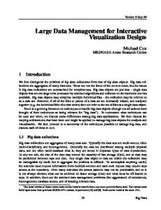
Table 2. Performance measurement for dynamic data sets: Comparison between SES and simplified SES (Simple). Name Fig. 11. A coupling protein (PDB-ID: 1GKI) which was used for performance measurements, colored by amino acid chain.
Recently, MetaMol, a GPU ray casting of the Molecular Skin Surface (MSS) [12], was presented by Chavent et al. [7]. Unlike the SES, the MSS is not defined by a rolling probe and only composed of quadric patches. The visual quality is analogous to our implementation. We compared the frame rate of our implementation to that of [7], using the identical data sets and the same hardware configuration (Intel CPU 2.4 GHz, NVIDIA Geforce 8800 GTX). For a protein of close to 2,000 atoms (PDB-ID: 1J4N, the largest data set used for testing MetaMol) they attained 7 fps while our method reached over 30 fps despite the higher cost for quartic root finding. This can be attributed to unoptimized rendering for the MSS, while our implementation was highly optimized for speed. As assumed, the frame rates for both methods exhibit linear scaling in respect of the number of atoms for small proteins. The preprocessing step for the MSS also induces considerably higher computational times compared to the SES, due to the construction of the mixed cells, which arise from a weighted Vorono¨ı diagram and a weighted Delaunay tetrahedralization. For the aforementioned protein of 2,000 atoms, MetaMol takes 15s for preprocessing, while our implementation takes less than 1s. Since MetaMol can currently be seen as a proof of concept, it offers no specific support for dynamic data and is therefore unserviceable for the use with trajectories. The following tests were done on an Intel Core 2 Duo 3 GHz with 4 GB RAM and an NVIDIA GeForce GTX280. The window size was set to 1024×1024 pixels and the proteins were fitted tightly into the ˚ screen. The probe radius was set to the canonical value of 1.4A. Table 1. Performance measurement for static data sets: SES without depth cues (w/o) and with Depth Darkening [24] (DD). RSS and STS denote the storage needed for the RS and the singularity texture. CT stands for the computation time for the RS. PDB-ID 1VIS 1AF6 1GKI 1AON
#Atoms
w/o (fps)
DD (fps)
SC (%)
RSS (MB)
STS (MB)
CT (s)
∼ 2,500 ∼ 10,000 ∼ 19,500 ∼ 59,500
60 27 19 13
49 24 17 12
60 70 70 55
0.7 2.8 5,4 18.5
0.3 1.2 3.1 10.4
0.08 0.36 0.77 2.68
In order to evaluate the rendering times and memory consumption of our ray casting implementation, we used several protein data sets from the PDB [3]. Table 1 shows the results of selected representative data sets. The mevalonate kinase 1VIS—displayed on the right in Fig. 1—with a chain length of about 300 amino acids represents an average sized protein (cf. Section 2.2). Since the data sets contain static data, no dynamic update of the RS was necessary for rendering
TEM β -lac (sim 1) TEM β -lac (sim 2) TEM β -lac (sim 2) TEM β -lac (sim 3) 8 × TEM β -lac CR lipase
RMSD yes yes no no no no
#Atoms
SES (fps)
Simple (fps)
∼ 4,060 ∼ 4,060 ∼ 4,060 ∼ 4,060 ×4,060 ∼ 8× ∼ 7,920
10–20 8–16 7–12 ∼5 – ∼2.5
∼55 ∼58 ∼56 ∼60 ∼5 ∼33
Different simulations of the same protein can lead to a higher number of moving atoms, resulting in lower frame rates. By applying RMSD alignment, a small but noticeable speedup is gained (cf. Table 2, sim 2). For trajectories with high dynamics (e.g. sim 3), the intended goal of 10 fps is just not achieved. Since the simplified SES is always completely recomputed in every frame, it is independent of the number of moving atoms. Therefore, the frame rates are equal for all trajectories of the same protein, as expected. Even for large proteins, interactive frame rates are easily attained when using the simplified SES. Only for the trajectory of 8 proteins, containing a total of more than 32,000 atoms, the frame rate drops considerably below 10 fps. We compared our approach to VMD [18], Chimera [29] and PyMOL [11], which use the program MSMS by Sanner [36] to compute the SES, like almost all available molecular viewers. The advantage of MSMS is that it is quite fast and offers a high-quality triangulation with arbitrary tessellation. However, the drawback is, that it cannot update the SES but recomputes it completely for every frame. Furthermore, even when using the standard parameters—resulting in a low tessellation—the triangulation generated by MSMS consumes twice the memory compared to the implicit representation used in our work, and roughly doubles the computation time. VMD additionally offers the possibility to use the program SURF by Varshney [41], which also cannot update the SES. Because PyMOL attempts to precompute the geometry of the SES for every frame of the whole trajectory, it is virtually not possible to view larger trajectories. Even when selecting very few frames (