1 JUNE 2003
FARRARA AND YU
1703
Interannual Variations in the Southwest U.S. Monsoon and Sea Surface Temperature Anomalies: A General Circulation Model Study JOHN D. FARRARA Department of Atmospheric Sciences, University of California, Los Angeles, Los Angeles, California
JIN-YI YU Department of Earth System Science, University of California, Irvine, Irvine, California (Manuscript received 12 June 2002, in final form 23 September 2002) ABSTRACT The interannual variability in the southwest U.S. monsoon and its relationship to sea surface temperature (SST) anomalies is investigated via experiments conducted with the University of California, Los Angeles, atmospheric general circulation model (AGCM). When the model is run without interannual variations in SSTs at the lower boundary, the simulation of the climatological mean monsoon is quite similar to the observed. In addition, the interannual precipitation variance and wet minus dry monsoon composite differences in the precipitation and monsoon circulation are largely realistic. When interannual variations in SSTs are introduced, the simulated interannual precipitation variance over the southwest U.S. monsoon region does not increase. Nor do SSTs seem to be important in selecting for wet or dry monsoons in this simulation, as there is little correspondence between observed wet and dry monsoon years and simulated wet and dry years. These results were confirmed through a 20-member ensemble of shorter seasonal simulations forced by an SST anomaly field corresponding to that observed for a wet minus dry southwest U.S. monsoon composite. When the AGCM is coupled to a mixed-layer ocean model, the pattern of SST anomalies generated in association with wet and dry monsoons is remarkably similar to that observed: there is a large area of positive SST anomalies in the subtropical eastern Pacific Ocean and weaker negative anomalies in the midlatitude North Pacific and Gulf of Mexico. It is demonstrated that the SST anomalies in the Pacific Ocean are forced by anomalies in the net surface solar radiative flux from the atmosphere associated with variations in planetary boundary layer stratus clouds; these variations are enhanced by a positive feedback between SST and stratus cloud variations. The anomalies in the Gulf of Mexico are associated with anomalous latent heat fluxes there. It is concluded that internal atmospheric variations are capable of 1) producing interannual variations in the southwest U.S. monsoon that are comparable to those observed, and 2) thermodynamically forcing the SST anomalies in the adjacent Pacific Ocean and Gulf of Mexico that are observed to accompany these variations. The implications of these results for seasonal forecasting are rather pessimistic since variations associated with internal atmospheric processes cannot be predicted on seasonal timescales.
1. Introduction The atmospheric circulation over North America during the summer season has many of the characteristics of a monsoon circulation (Tang and Reiter 1984). This circulation has been labeled the ‘‘North American monsoon system’’ (NAMS) by Higgins et al. (1997), who give a description of its life cycle in terms of development, mature, and decay phases. The development phase that occurs during May and June is characterized by the following Corresponding author address: Dr. John D. Farrara, Department of Atmospheric Sciences, Mail Code 156505, University of California, Los Angeles, Los Angeles, CA 90095-1565. E-mail:
[email protected]
q 2003 American Meteorological Society
circulation changes: the extratropical storm track weakens and shifts poleward, the frequency of occurrence and intensity of the Great Plains low-level jet increases, and over southwest Mexico monsoon rains and the upper-tropospheric monsoon high develops. The mature phase during July and August is characterized by the strengthening and northward migration of the monsoon high into the southwestern United States and an extension of the monsoon rains northward into northwest Mexico and the southwestern United States. The decay phase (September–October) is characterized by a gradual weakening and southward migration of the monsoon high and diminished monsoon rainfall throughout the region. The NAMS can exert a significant control over summer rainfall throughout a large portion of the United States and
1704
JOURNAL OF CLIMATE
Mexico. In the United States, this control is often manifested as an out-of-phase relationship between rainfall in the Southwest and Great Plains and an in-phase relationship between the Southwest and the East Coast (Mo et al. 1997; Higgins et al. 1997). Thus, before the onset of monsoon rainfall in the southwestern United States, rainfall is enhanced over the Great Plains and suppressed along the East Coast. After the onset of monsoon rainfall in the southwest, rainfall is suppressed over the Great Plains and enhanced along the East Coast (Tang and Reiter 1984; Douglas et al. 1993; Mock 1996; Okabe 1995). The North American summer monsoon circulation exhibits substantial interannual variability. This variability has important impacts on hydrological resources in the southwestern United States and potentially throughout the country via its relationships with the Great Plains and East Coast. Wet (dry) monsoons in the southwestern United States are accompanied by an intensified and northeastward-shifted (suppressed and southward shifted) monsoon anticyclone in the upper troposphere (Carleton et al. 1990; Higgins et al. 1998). During dry monsoons much of the Mississippi Valley, Ohio Valley, and mid-Atlantic states tend to be wetter than normal. In particular, the recent notable Midwest summer flood (drought) events of 1993 (1988) occurred during seasons characterized by dry (wet) monsoons. In summary, the intensity and position of the monsoon anticyclone seems to be one of the fundamental controlling factors on summertime rainfall in large parts of the United States. Determining causes and effects in this relationship, however, is complicated by the fact that in some cases—the 1988 drought in particular—the rainfall anomalies in the Midwest preceded those in the monsoon circulation. On timescales longer than about 10 days, the processes that produce fluctuations in atmospheric circulation patterns can be broadly divided into two classes. One class can be labeled ‘‘external’’ forcing from the lower boundary. These slowly varying boundary conditions include sea surface temperatures (SST), soil moisture, and snow cover. The SST anomalies associated with El Nin˜o and La Nin˜a events are a prominent example of this type of forcing (Deser and Blackmon 1993). The second class is related to internal dynamical processes in the atmosphere. In this class, variations are produced without any variations in the external forcing. Interactions among different components of the atmospheric circulation (tropical–extratropical or wave– mean flow interactions) cause the circulation to vacillate between different regimes (e.g., Charney and DeVore 1979; Yu and Hartmann 1993). For the extratropical winter circulation, several studies have suggested that these two classes of processes are roughly comparable in importance in producing interannual variations in the circulation (Brankovic et al. 1994; Kumar and Hoerling 1997). Fewer studies have been performed for the summer season. The relative importance of these two classes of processes has clear implications for seasonal forecasting since the variations associated with internal dy-
VOLUME 16
namical processes in the atmosphere cannot be predicted on seasonal timescales. Thus far, establishing clear links between interannual variations in the intensity and position of the monsoon anticyclone and the slowly varying lower boundary conditions (SSTs, soil moisture, and snow cover) has proven difficult. Concerning tropical SST anomalies, Higgins et al. (1999) did not find a clear relationship between El Nin˜o/La Nin˜a and monsoon rainfall in northwest Mexico and the southwestern United States, although they identified a weak association between dry monsoons in the southwestern United States (northwest Mexico) and La Nin˜a (El Nin˜o). Other studies on El Nin˜o/La Nin˜a relationships to monsoon rainfall in the southwest United States show no clear consensus: Andrade and Sellers (1988) found little correlation between El Nin˜o/La Nin˜a events and total summer rainfall in New Mexico and Arizona, while Harrington et al. (1992) suggested that there is a relationship between these events and the geographic distribution of precipitation in the region. Higgins et al. (1999) did, however, find that monsoon rainfall in southwest Mexico is modulated by the SST anomalies associated with El Nin˜o and La Nin˜a, such that wet (dry) monsoons are almost always associated with La Nin˜a (El Nin˜o). They attributed this, in part, to the impact of local SST anomalies on the land–sea thermal contrast (and, therefore, monsoon strength). Using a composite analysis of wet minus dry monsoon years, Higgins et al. (1999) showed that the pattern of SST anomalies associated with anomalous monsoon rainfall in the southwestern United States and northwest Mexico is quite different from that of a composite La Nin˜a minus El Nin˜o pattern of SST anomalies. In particular, the anomalies along the west coast of North America are of opposite sign in the two composites. Their wet minus dry composite for the southwestern United States shows negative anomalies in a band along 408N in the Pacific east of the date line with positive anomalies to the south and east that are strongest along the coast of Baja California and weak negative anomalies in the Gulf of Mexico. It has also been shown that wet (dry) monsoons in the southwest United States tend to follow winters that were wetter (drier) than normal in the Pacific Northwest and drier (wetter) than normal in the southwest United States (Carleton et al. 1990; Higgins et al. 1998). Both Carleton et al. and Higgins et al. suggested that the influence of the previous winter was through the persistence of SST anomalies established during the preceding winter in the extratropical Pacific adjacent to the region. However, it is also possible that the SST anomalies in this region observed in association with wet and dry monsoons are forced by the atmosphere. Recent observational (Gutzler and Preston 1997) and regional modeling (Small 2001) studies have suggested that anomalies in snow cover/ soil moisture in the Great Basin/Rocky Mountains could supply the required ‘‘memory’’ to produce such
1 JUNE 2003
FARRARA AND YU
a relationship between winter and summer rainfall. The mechanism of influence on the monsoon in this case would be through a decrease (increase) in the land–sea temperature contrast, and thus monsoon strength, in years with anomalously high (low) snow cover. These studies are limited, however, by a relative scarcity of land surface data available for verification. Further clouding the picture is a recent observational study (Kim 2002) using a century-long precipitation dataset that has called into question the robustness of the relationship between summer and winter precipitation in the southwest United States. In the dataset Kim analyzed, dry (wet) winters preceded wet (dry) summers in the southwest United States only after about 1960. In summary, the role played by the slowly varying lower boundary conditions in the interannual variability of the monsoon is not very clear and there remains the possibility that a substantial portion of its interannual variability is due to dynamical processes internal to the atmosphere. Determining the relative roles of ‘‘internal’’ and lower boundary forcing processes in producing interannual variability in the monsoon is a major objective of the current study. In particular, we focus on the interannual variability in the southwest United States. Given the uncertainties associated with land surface processes, and the possibilities for interactions between land surface variability and variability forced by SSTs, we have chosen to focus on the internal variability and the variability associated with SST anomalies at this stage. For this work, we use a methodology based on experiments conducted using a global climate model, the University of California, Los Angeles (UCLA) atmospheric general circulation model (AGCM). Simulating monsoon rainfall using global atmospheric models has proven difficult. For example, Yang et al. (2001) analyzed the National Center for Atmospheric Research Community Climate Model 3 (NCAR CCM3) in this regard and found that regardless of the land surface model used, the CCM3 underestimates the observed summer rainfall in Arizona–New Mexico by a factor of 5 or more. Possible reasons for this difficulty include the complex topography of the region and the multiple sources of moisture and the relatively small scales involved. However, as demonstrated by Boyle (1998) in a comparison of Atmospheric Model Intercomparison Project (AMIP) model simulations of Arizona–New Mexico rainfall, use of higher model resolution is not sufficient to produce a superior simulation. We demonstrate below a successful simulation of the NAMS by the UCLA AGCM that we use as the starting point for a set of experiments designed to characterize the natural interannual variability of the simulated southwest U.S. monsoon and to investigate the impact, if any, of SSTs on its interannual variations. In the following section, we describe the version of the UCLA AGCM used and the design of the two primary 20-yr integrations we
1705
analyze, one CONTROL and one AMIP-type simulation. In section 3, we examine the climatology and interannual variability of the monsoon in these two simulations. In an attempt to better understand (and establish the statistical significance of) the results obtained in section 3, we present and analyze in section 4 an ensemble of seasonlong simulations. Section 6 contains a discussion and our conclusions. To explore further the origin of extratropical SST anomalies adjacent to the southwest U.S. monsoon region, we analyze in an appendix the results of an extended integration in which the AGCM is coupled to a simple thermodynamic mixed-layer ocean model in the extratropics. 2. Description of the UCLA AGCM and design of the experiments The UCLA AGCM is a comprehensive gridpoint model of the global atmosphere extending from the earth’s surface to the top of the stratosphere (50 km). The model is based on the primitive equations, with horizontal velocity, potential temperature, surface pressure, water vapor mixing ratio, cloud water mixing ratio, cloud ice mixing ratio, ground temperature, and snow depth over land as the model’s prognostic variables. The model equations are discretized using an Arakawa C grid in the horizontal (Arakawa and Lamb 1977; Arakawa 1981) and a modified sigma coordinate in the vertical (Arakawa and Suarez 1983; Suarez et al. 1983). The model includes advanced parameterizations of the major physical processes in the atmosphere including solar and terrestrial radiation (Harshvardhan et al. 1987, 1989), cumulus convection, and planetary boundary layer processes. A prediction scheme for cloud liquid water and ice based on a five-phase bulk microphysics is used (Ko¨hler 1999) and cloud radiative properties are computed based on these water and ice mixing ratios. An important aspect of this scheme is that the decay timescale for cloud ice takes into account the fact that air inside clouds is generally convective. The parameterization of cumulus convection is a version of the Arakawa–Schubert scheme (Arakawa and Schubert 1974) in which the cloud work function quasi equilibrium is relaxed by predicting the cloud-scale kinetic energy (Pan and Randall 1998) and that includes the effects of convective downdrafts (Cheng and Arakawa 1997). This parameterization is intimately linked to the parameterization of planetary boundary layer processes that follows the mixed-layer approach of Suarez et al. (1983) as modified by Li et al. (1999) and Li et al. (2002); the recent modifications result in improved simulations of stratocumulus cloud incidence and surface solar radiative fluxes. At the earth’s surface, monthly mean values of the SST and sea ice extent (Rayner et al. 1995), albedo, ground wetness, and roughness length (Dorman and Sellers 1989) are prescribed. Daily values of these surface conditions are determined from the monthly mean values by linear interpolation. The surface temperature over land is predicted using the predicted snow depth and a prescribed albedo and surface heat capacity in a
1706
JOURNAL OF CLIMATE
VOLUME 16
simple surface energy balance calculation. All the simulations presented here use a model resolution of 2.58 longitude, 28 latitude with 29 levels in the vertical. The model has been shown to quite accurately simulate the major time-averaged features of the global atmospheric circulation (Suarez et al. 1983; Kim et al. 1998). In addition, the response of the model atmosphere during northern winter to the tropical SST anomalies that characterized the 1997/98 El Nin˜o event has been analyzed (Farrara et al. 2000) and found to be quite realistic. In section 3, we examine the model’s performance in simulating the North American monsoon. To investigate the origins of SST anomalies adjacent to the NAMS region we also couple the AGCM to a constant-depth mixed-layer ocean model (see the appendix). This mixed-layer ocean has a constant depth of 50 m and its temperature (SST) is determined by the net fluxes of heat at the air–sea interface (as determined by the AGCM) and a flux that represents the ocean advective heat flux. This ocean advective heat flux is determined as the residual in a simple heat balance equation for the mixed layer using the heat fluxes at the ocean surface from the CONTROL AGCM simulation and the prescribed month-to-month changes in SST used in that simulation. To begin our investigation of the relative roles of internal and lower boundary forcing processes in producing interannual variability in the monsoon we performed two 20-yr-long AGCM simulations. The first simulation uses the Global Sea Ice and Sea Surface Temperature dataset (GISST) climatological SSTs (Rayner et al. 1995; averaging period: 1960–90) and the second uses observed SSTs [for the period 1979–98, in which anomalies taken from the Reynolds SST dataset (Smith and Reynolds 1998) were added to the GISST climatology]. We refer to these simulations as CONTROL and AMIP, respectively. In both of these simulations, land surface conditions are prescribed as described above. In the following section, the patterns and magnitude of the interannual variability in the NAMS found in the CONTROL simulation are analyzed and compared to observations of NAMS variability and to that found in the simulation that includes SST anomalies. The observed datasets we use are 1) precipitation estimates from the Climate Prediction Center’s Merged Analysis of Precipitation (CMAP; Xie and Arkin 1997) and 2) 200-hPa geopotential heights from the (National Centers for Environmental Prediction) NCEP–NCAR reanalysis (Kalnay et al. 1996). The design of the ensembles of season-long simulations and the extended integration using the AGCM coupled to a constant-depth mixed-layer ocean model are described in more detail in sections 4 and 5, respectively.
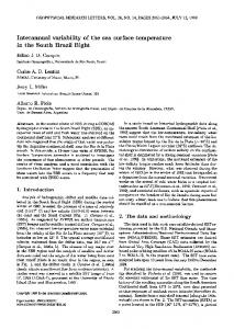
FIG. 1. Climatological precipitation rate (mm day 21 ) averaged over the months of JAS from (a) the CMAP (1979–98), (b) the CONTROL simulation of the UCLA AGCM, and (c) the AMIP simulation of the UCLA AGCM. The contour interval is 1 mm day 21 . Light shading indicates areas with greater than 2 mm day 21 and heavy shading areas with greater than 5 mm day 21 .
3. Simulated interannual variability in the CONTROL and AMIP simulations a. Simulated climatology—CONTROL As mentioned in the introduction, simulating North American summer monsoon rainfall using global at-
mospheric models has proven difficult. Therefore, we examine first the performance of the UCLA AGCM in this regard. Figure 1 shows the 20-yr mean precipitation for the summer season [July–August–September (JAS)] over Mexico, the United States, southern Canada, and
1 JUNE 2003
FARRARA AND YU
FIG. 2. Month-by-month evolution of the climatological precipitation rate (mm day 21 ) in AZ–NM (box boundaries: 318–378N, 1028– 1148W). The dashed line shows values from the CMAP, the solid line values from the AGCM CONTROL simulation, and the dotted line values from the AGCM AMIP simulation.
adjacent ocean areas from the CONTROL simulation and the 1979–98 JAS mean from the CMAP data. The overall pattern and absolute values from the simulation are in broad agreement with the CMAP observations. In particular, in the CONTROL simulation (Fig. 1b) there is abundant monsoon rainfall in a realistic pattern of high values along the Pacific coast of Mexico that extends northward with diminished intensity along the Sierra Madre Occidental range into northwest Mexico and the southwestern United States. There are, however, areas of significant model error, such as the Pacific Northwest, where precipitation is overestimated. Figure 2 shows the month-to-month evolution of the precipitation rate in Arizona–New Mexico (AZ– NM; 318–378N, 1028–1148W). Precipitation in this region in the CONTROL simulation is overestimated throughout the year. This overestimate is most serious (greater than 1 mm day 21 ) during the first 5 months of the year. During the rest of the year—including the entire summer season—the overestimate ranges from 0.5 to 0.75 mm day 21 . For the JAS mean, the CONTROL overestimates precipitation by a factor of about 1.4. The simulated evolution is quite realistic with a relative minimum in the spring (the model’s minimum is in May, the observed is in April), a dramatic increase in July at monsoon onset, and then a slower decrease in September–October as the monsoon decays. Figure 3 shows the changes in precipitation outside the AZ–NM monsoon region associated with this onset by presenting a map of the July minus June precipitation for the same region as shown in Fig. 1. This figure can be directly compared with the corresponding observed data shown in Fig. 8 of Higgins et al. (1997). Though there are some differences in the magnitude, all the major features of the continental-
1707
scale mode of variability pointed out by Higgins et al. are reproduced in the CONTROL simulation. Specifically, we note the increases in precipitation over AZ–NM, the decreases surrounding this area to the north and east, and the increases in the eastern part of the United States. The simulation of the upper-tropospheric anticyclone associated with the NAMS is also similar to that observed. Figure 4 shows the zonally asymmetric part of the JAS mean 200-hPa geopotential height fields from the NCEP– NCAR reanalysis (Kalnay et al. 1996) and the CONTROL simulation (Figs. 4a and 4b, respectively). Both fields show positive values over northern Mexico and most of the middle part of the United States, reflecting the monsoon anticyclone, in the CONTROL this anticyclone; is somewhat stronger than and located somewhat southwest of the observed one. The simulated climatological fields from the AMIP integration are nearly identical to those shown here for the CONTROL. We conclude that the UCLA AGCM simulation of the North American monsoon is largely realistic, thus satisfying a necessary prerequisite for its use in our subsequent sensitivity studies of interannual variability in the NAMS. b. Simulated interannual variability—CONTROL Since albedo, ground wetness, and SSTs were prescribed from a climatology, there is virtually no external forcing of interannual variability in the CONTROL integration. The year-to-year fluctuations in the NAMS found in this simulation must be associated with the internal variability of the atmospheric circulation. We examine first the magnitude of this interannual variability by computing the interannual variance in precipitation and comparing it to that observed. Figure 5 shows the interannual standard deviation in the seasonal (JAS) mean precipitation over monsoon region from CMAP observations (Fig. 5a) and the CONTROL integration (Fig. 5b). In the core monsoon region in Mexico, the simulated and observed standard deviations are similar in magnitude over land, while the simulated interannual variability is substantially smaller over the adjacent Pacific Ocean. The variability over the continental United States tends to be somewhat smaller than that observed and is approximately 75% of that observed in AZ–NM. This reduced variability is expected in a simulation without variations in land surface conditions, as these have been shown (e.g., Koster and Suarez 1995; Koster et al. 2000) to be a significant enhancer of precipitation variance over the Northern Hemisphere midlatitude land areas during the summer season, though not a major contributor in the southwest United States. We examine next differences between composites of ‘‘wet’’ and ‘‘dry’’ monsoons in the southwest United States. The years included in the observed composites (see figures) are the same as those presented in Higgins et al. (1999) for his AZ–NM averaging region (328–368N, 112.58–107.58W) and chosen by selecting years with JAS precipitation of more (less) than 0.5 standard deviations above (below) the cli-
1708
JOURNAL OF CLIMATE
VOLUME 16
FIG. 3. Climatological Jul minus Jun precipitation (mm day 21 ) from (a) the CONTROL simulation and (b) the AMIP simulation. The contour interval is 0.5 mm day 21 . Light shading indicates areas with differences of less than 21 mm day 21 and heavy shading areas with differences greater than 1 mm day 21 .
matological values as wet (dry) monsoons. The years included in the composites from the AGCM simulations were chosen based on the area-averaged precipitation in AZ–NM. The four years (out of 20) with the largest precipitation were assigned to the wet composite and the four years with the smallest precipitation were assigned to the dry composite. Since the SSTs used are from a climatology, the years in the CONTROL simulation are simply numbered sequentially starting at year 1. Figure 6 compares the observed (CMAP) precipitation composite of wet minus dry monsoon years with a similar composite constructed from the 20-yr CONTROL simulation. The magnitude of the wet minus dry differences in AZ– NM and parts of Mexico in the CONTROL are very similar to those observed. The maximum positive dif-
ferences are between 0.75 and 1 mm day 21 in both cases; however, in the CONTROL composite the maximum differences are centered in New Mexico, while in the observed composite the center is in Arizona. Wet minus dry differences in other areas of the United States and Mexico show less agreement. In particular, although there are weak negative differences in the upper Great Plains in CONTROL, the large area of observed negative differences in the Great Plains and Mississippi Valley (representing the out-of-phase between rainfall in the Southwest and Great Plains emphasized by Higgins et al. 1997) are not reproduced in CONTROL. It is not clear how important this failing is, especially in light of the recent analysis of a century-long rainfall dataset by Kim (2002), which calls into question the robustness of this out-of-phase
1 JUNE 2003
FARRARA AND YU
1709
to that observed. However, the simulated height changes tend to be more zonally symmetric than those observed with height increases at all longitudes between 258 and 508N and decreases poleward, reflecting an intensification of the summertime subpolar storm track and jet stream. In summary, the simulation of the interannual variability in the NAMS in the CONTROL simulation is largely realistic, suggesting that internal atmospheric processes alone might account for the observed variability. In anticipation of how atmospheric circulation differences might force sea surface temperature anomalies in the regions adjacent to the monsoon, we plot in Fig. 8 the wet minus dry composites of the surface latent heat flux from the CONTROL simulation (Fig. 8a) and net surface fluxes (Fig. 8b).1 Figure 8a shows that latent heat fluxes (evaporation) are greater during wet monsoons in both the Gulf of Mexico and off the Baja California coast south of 258N. Therefore, latent heat fluxes in these two regions would tend to cool the ocean surface more during wet monsoons. However, in the Pacific the net surface fluxes (into the ocean, Fig. 8b) actually increase off the Baja California coast in wet monsoons compared to dry monsoons. This increase is almost entirely due to increases in surface solar radiative fluxes associated with the decreases in stratus clouds (not shown) that overwhelm the impact of the increased latent heat fluxes there. To the northwest of this region in the midlatitude North Pacific, stratus clouds increase, and net surface fluxes and surface solar fluxes decrease. In the Gulf of Mexico, the decrease in net surface fluxes is due to the increase in latent heat fluxes there shown in Fig. 8a. We will revisit these differences in section 5 when we explore the origins of the sea surface temperature anomalies observed in association with wet and dry monsoons. FIG. 4. Climatological deviations from the zonal mean of the 200hPa geopotential height fields (m) averaged over JAS from (a) the NCEP–NCAR reanalysis (1968–96), (b) the CONTROL simulation, and (c) the AMIP simulation. The contour interval is 20 m and the zero contour is omitted. Light shading indicates areas with values less than 260 m and heavy shading areas with values greater than 40 m.
relationship between the southwest United States and Great Plains/Mississippi Valley. Figure 7 shows the observed and CONTROL wet minus dry composite 200-hPa geopotential heights. As shown by Carleton et al. (1990), Higgins et al. (1998), and Fig. 7a, wet (dry) monsoons in the southwestern United States are observed to be accompanied by an intensified and northward-shifted (suppressed and southward shifted) monsoon anticyclone in the upper troposphere. In the CONTROL composite (Fig. 7b), there is an intensification and northward shift of the monsoon anticyclone that is similar in magnitude
c. Simulated interannual variability—AMIP We examine first the magnitude of the interannual variability by computing the interannual variance in precipitation and comparing it to that in the CONTROL simulation. Figure 9 shows the difference (AMIP 2 CONTROL) in the interannual standard deviation in the seasonal (JAS) mean precipitation over monsoon region. The addition of year-to-year variations in SSTs results in slight decreases in the interannual variations in precipitation nearly everywhere in the United States, including AZ– NM. The variability increases somewhat over the core monsoon region in Mexico and the eastern Pacific Ocean adjacent to this region and over the Gulf of Mexico and adjacent land areas (e.g., Florida). The increases in variability over Mexico result in values there that are larger 1 Note that in Fig. 8b, the sign of the fluxes is the opposite of that in Fig. 8a, and is such that positive values indicate a tendency of the atmosphere to warm the underlying ocean.
1710
JOURNAL OF CLIMATE
VOLUME 16
FIG. 5. Interannual standard deviation (mm day 21) in precipitation averaged over JAS from (a) the CMAP (1979–98) and (b) the CONTROL simulation of the UCLA AGCM. The contour interval is 0.25 mm day21. Shading indicates areas with standard deviations greater than 1 mm day 21.
than observed. It must be noted, however, that none of these differences are statistically significant. We have also constructed composites of wet and dry monsoons in the same way as was done for the CONTROL simulation. In this case the years given for the AMIP simulation correspond to particular years during the period 1979–98 since observed SSTs for this period were used. Figure 10 shows the precipitation composite from the AMIP simulation. Figure 10 shows a rather different pattern of wet minus dry differences than that found in the CONTROL simulation (Fig. 6). The maximum positive differences in the southwest United States are somewhat smaller (consistent with the smaller interannual variability found there) and the values throughout the rest of the United States are mostly small
and positive. The pattern throughout the rest of the United States, as well as differences in the 200-hPa height field and other dynamical fields (not shown), are also in general less similar to the observed than those obtained in the CONTROL simulation. In addition, it seems that SSTs are not playing an important role in ‘‘selecting’’ wet or dry years; there is little correspondence between observed wet and dry monsoon years and the wet and dry monsoons in the AMIP simulation. In fact, three of the four dry monsoon years in the simulation (1984, 1986, and 1988) were observed to be wetter than normal (see Fig. 6a). In summary, we do not find a systematic impact of SST anomalies on the monsoon in the AMIP simulation. We consider three possible explanations for this result: 1) the
1 JUNE 2003
FARRARA AND YU
1711
FIG. 6. Composite wet minus dry precipitation differences (mm day 21 ) averaged over JAS for (a) the CMAP (1979–98) and (b) the CONTROL simulation of the UCLA AGCM. Years included in the composites are listed below each panel. The contour interval is 0.25 mm day 21 , negative contours are dashed, and the zero contour is omitted. Light shading indicates areas with differences less than 20.75 mm day 21 and heavy shading areas with differences greater than 0.75 mm day 21 .
single realization of each year in the AMIP simulation is not sufficient to distinguish the SST-forced signal from the ‘‘natural variability,’’ which, according to our CONTROL simulation, is large; 2) the natural atmospheric variability is the driver and atmospheric circulation anomalies are thermodynamically forcing SST anomalies adjacent to the monsoon region rather than vice versa; and 3) land surface processes are playing a mediating role in the relationship between SSTs and monsoon variability. We examine hypotheses 1 and 2 in the following section and the appendix, respectively.
4. The impact of SST anomalies To address hypothesis 1 we have performed two 20-member ensembles of integrations for the summer season (May–September). The large ensembles allow us to determine the statistical significance of changes in the atmospheric circulation that develop in response to the SST anomalies imposed in the second ensemble. One is an analog to CONTROL in that it uses climatological SSTs. This ensemble was run to provide a large sample of independent realizations of the control climate from which to assemble random
1712
JOURNAL OF CLIMATE
VOLUME 16
FIG. 7. Composite wet minus dry JAS 200-hPa geopotential height differences (m) from (a) the NCEP–NCAR reanalysis and (b) the CONTROL run of the UCLA AGCM. Years included in the composites are given below each panel. The contour interval is 5 m, negative contours are dashed, and the zero contour is omitted. Light shading indicates areas with differences less than 215 m and heavy shading areas with differences greater than 15 m.
combinations for the Monte Carlo significance testing. The 20 different initial conditions were constructed by adding small random perturbations to the model’s prognostic variables corresponding to an atmospheric state realized on 1 May of year 10 in the 20-yr CONTROL run. The other ensemble is forced by a global SST anomaly field (Smith and Reynolds 1998) derived from an observed composite of wet minus dry monsoon years in AZ–NM (see Fig. 11) using the same set of perturbed initial conditions as used for the CONTROL ensemble. The years in this wet minus dry composite are the same as those shown
in Fig. 8a. Figure 11 shows that this SST anomaly field is characterized by positive anomalies approaching 1 K in the subtropical eastern Pacific Ocean immediately adjacent to the monsoon region with weaker negative anomalies in the midlatitude North Pacific and Gulf of Mexico. In the tropical Pacific Ocean, which is outside the domain plotted in Fig. 11, there are weak negative anomalies in the eastern equatorial region, suggesting a slight preference for wet monsoons during La Nin˜a years. Figure 12 shows the ensemble mean difference in JAS precipitation in the CONTROL and anomaly ensembles.
1 JUNE 2003
FARRARA AND YU
1713
FIG. 8. Composite wet minus dry JAS differences in the CONTROL run of (a) surface latent heat fluxes (W m 22 ) and (b) net surface fluxes (W m 22 ). Note that in (b) a slightly larger domain is plotted and the sign is opposite that in (a), and is such that positive (negative) values indicate a tendency of the atmosphere to warm (cool) the ocean. Years included in the composites are given below each panel. The contour interval is 10 W m 22 , negative contours are dashed, and the zero contour is omitted. Light shading indicates areas with differences less than 220 W m 22 and heavy shading areas with differences greater than 20 W m 22 .
We note first that the difference pattern does not look much like the observed or CONTROL wet minus dry precipitation difference patterns shown in Fig. 6. In Mexico there is an increase in precipitation in the northwest part of the country—the region adjacent to the positive SST anomalies in the Pacific Ocean—and decreases elsewhere. There are also decreases over the Gulf of Mexico—where negative SST anomalies were prescribed—and Florida. The differences over the rest of the continental United States (including the southwest
monsoon region) are very small. In particular, there are small decreases in precipitation in AZ–NM even though the anomaly ensemble is forced with SST anomalies observed when precipitation there is greater than normal. The statistical significance of these results was determined via Monte Carlo methods (Livezey and Chen 1983; Livezey 1985). The areas in Fig. 12 where the differences between the two ensembles are significant at the 95% level are shown by gray shading. This shading covers only a small region in northwest Mexico,
1714
JOURNAL OF CLIMATE
VOLUME 16
FIG. 9. Difference (AMIP minus CONTROL) in interannual standard deviation (mm day 21 ) in precipitation averaged over JAS. The contour interval is 0.25 mm day 21 .
none of the other differences in Fig. 12 are significant at this level, and there is certainly no field significance. In addition, the ensemble mean anomaly–CONTROL differences in 200-hPa geopotential heights (not shown) are relatively small (and not significant) and have a pattern that is very different from the observed and CONTROL wet minus dry differences shown in Fig. 7. In particular, the differences are negative over the monsoon region rather than positive; the monsoon anticyclone is suppressed in the anomaly run. This analysis suggests that, both hydrologically and dynamically, there is no systematic impact of the SST anomalies on the atmospheric circulation over North America during summer in the AGCM. In fact, although the differences are not statistically significant, the precipitation in the southwest United States actually decreases in the anomaly ensemble compared to the CONTROL ensemble, suggesting that hypothesis 1 cannot explain the lack of correspondence between observations and the results of the AMIP simulation. Koster et al. (2000) reached a similar conclusion, noting that in their simulations, SSTs contribute the most to precipitation variance in the Tropics, whereas chaotic atmo-
← FIG. 10. Composite wet minus dry JAS differences in (a) precipitation (mm day 21 ) and (b) 200-hPa heights (m) from the AMIP run. Years included in the composites are given below each panel. In (a) the contour interval is 0.25 mm day 21 , negative contours are dashed, and the zero contour is omitted. Light shading indicates areas with differences less than 20.75 mm day 21 and heavy shading areas with differences greater than 0.75 mm day 21 . In (b), the contour interval is 5 m, negative contours are dashed, and the zero contour is omitted. Light shading indicates areas with differences less than 215 m and heavy shading areas with differences greater than 15 m.
1 JUNE 2003
FARRARA AND YU
1715
FIG. 11. Observed wet minus dry composite of Reynolds SST anomalies (K). Years included in the composites are listed below the figure. The contour interval is 0.25 K, negative contours are dashed, and the zero contour is omitted. Light shading indicates areas with differences less than 20.5 K and heavy shading areas with differences greater than 0.5 K.
spheric dynamics contribute most in the extratropics. We examine hypothesis 2 in the appendix. 5. Summary and discussion We have examined the interannual variability of the southwest U.S. monsoon with the objective of determining the relative roles of internal and lower boundary forcing processes in this variability. In view of the limitations in observing land surface conditions and the possibilities for interactions between land surface variability and interannual variability associated with SSTs, we have chosen to focus on the internal variability and the variability associated with SST anomalies in this paper. For this work, we used a methodology based on experiments conducted using a global climate model, the UCLA atmospheric general circulation model (AGCM). There were two primary 20-yr integrations we analyzed, one CONTROL that used climatological SSTs and one AMIP-type simulation that used observed SSTs for the period 1979–98. In both of these simulations land surface conditions, except for the ground temperature, are prescribed from a monthly varying climatology. We first confirmed that UCLA AGCM’s CONTROL simulation of the climatological monsoon is realistic enough to proceed with an analysis of the interannual variability. We examined the climatological monsoon precipitation, its June–July change, and the 200-hPa height field. For these fields we found that the simulated JAS climatology is realistic to a significantly greater degree than recently published simulations with other GCMs. As indicated in the introduction,
this result is not likely due to resolution; the resolution we use here is very similar to that used by many of the AMIP models (the horizontal resolution we use here is approximately equal to T42). Rather, we speculate that it is a result of the unique parameterization of planetary boundary layer (PBL) processes and the linkages between the PBL and convection parameterizations in the model. Together they generally produce a faithful representation of the diurnal cycle over land areas, which is of great importance in simulating the monsoon. We then compared the CONTROL-simulated and observed interannual variability and examined composites of wet minus dry monsoons. An analysis of the interannual variance in the JAS mean precipitation and the wet minus dry monsoon composite differences in precipitation and 200-hPa geopotential heights in the CONTROL simulation showed them to be largely realistic. At this point, we tentatively concluded that large-scale internal atmospheric processes alone might account for the observed variability. We next examined, in two different ways, the impact of SSTs. First, we compared the interannual variability in the AMIP simulation to that in the CONTROL. We found that the interannual precipitation variance over the southwest U.S. monsoon region does not increase. Nor did SSTs seem to be important in selecting for wet or dry monsoons in this simulation as there is little correspondence between observed wet and dry monsoon years and wet and dry years in this simulation. In fact, three of the four dry monsoon years in this simulation. (1984, 1986, and 1988) were observed to be wetter than normal.
1716
JOURNAL OF CLIMATE
VOLUME 16
FIG. 12. Anomaly minus CONTROL JAS ensemble mean difference in precipitation (mm day 21 ). The contour interval is 0.25 mm day 21 , negative contours are dashed, and the zero contour is omitted. The shaded region covers areas in which the differences are significant at the 95% level according to a Monte Carlo–type test (see text for details).
We considered three hypotheses for why this might be the case: 1) the single realization of each year in the AMIP simulation is not sufficient to distinguish the SSTforced signal from the natural variability (noise), which, according to our CONTROL simulation, is substantial; 2) the natural atmospheric variability is the driver and atmospheric circulation anomalies are thermodynamically forcing SST anomalies adjacent to the monsoon region rather than vice versa; and 3) land surface processes are playing a significant mediating role in the relationship between SSTs and monsoon variability. Examining hypothesis 1 led to the second way in which we investigated the impact of SST anomalies: through a 20-member ensemble of simulations for the summer season (May through September) forced by an SST anomaly field corresponding to that observed for a wet minus dry southwest U.S. monsoon composite. In this set of simulations we found no systematic impact of the SST anomalies on the atmospheric circulation over North America during summer. In fact, although the differences were not statistically significant, the precipitation in the southwest United States actually decreased in the anomaly ensemble compared to the CONTROL ensemble, suggesting that hypothesis 1 cannot explain the lack of correspondence between observations and the results of the AMIP simulation. These results are consistent with previous other climate model studies of precipitation variance (e.g., Koster et al. 2000) that have shown that SSTs are not a dominant factor in forcing precipitation variance outside the Tropics. In the appendix we investigate hypothesis 2 by performing another 20-yr integration, this time with the AGCM coupled to a (constant depth) mixed-layer ocean model. We find that wet minus dry southwest U.S. mon-
soon composites from this integration feature SST anomalies that are remarkably similar to those from the observed composite (though they tend to be larger than observed): there are large areas of positive SST anomalies in the subtropical eastern Pacific Ocean and weaker negative anomalies in the midlatitude North Pacific and Gulf of Mexico. The SST anomalies in the Pacific Ocean are forced by anomalies in the net surface solar radiative flux from the atmosphere associated with variations in PBL stratus clouds, which were enhanced by a positive feedback between SST and stratus cloud variations. The anomalies in the Gulf of Mexico are associated with anomalous latent heat fluxes there. We conclude that internal atmospheric variations are capable of 1) producing interannual variations in the southwest U.S. monsoon that are comparable to those observed, and 2) thermodynamically forcing the SST anomalies in the adjacent Pacific Ocean and Gulf of Mexico that are observed to accompany these variations. We note that the implications of these results for seasonal forecasting are rather pessimistic since variations associated with internal atmospheric processes are generally not predictable on seasonal timescales. Finally, we reiterate that all the results presented here were obtained with a model configuration in which land surface conditions (in particular, ground wetness and albedo) were prescribed from a climatology (noninteractive land surface with no interannual variations). Although there is no strong evidence in the literature to suggest that variations in land surface conditions are a primary driver of interannual variability in summer precipitation in midlatitude areas (Koster et al. 2000), there remains the possibility (see our hypothesis 3 above) that land surface processes are playing a significant mediating role in the re-
1 JUNE 2003
FARRARA AND YU
lationship between SSTs and summer monsoon precipitation. As we have confined this part of our study to an exploration of the impact of SSTs, this hypothesis remains unexamined here but is being examined using the UCLA AGCM coupled to the NCEP/Oregon State University/Air Force/National Weather Service Hydrologic Research Lab (NOAH) land surface model as part of our continuing work on this topic. In addition, our results were obtained with a single global climate model. To strengthen our conclusions, the experiments should be repeated with different global climate models. We plan to undertake such experiments when community climate models that can realistically simulate the North American monsoon become available. Acknowledgments. The authors gratefully acknowledge the assistance of Ms. Ying Teng in the analysis of the CONTROL and AMIP simulations and in the preparation of some of the figures. The authors also acknowledge the contribution of Dr. Jinwon Kim to this research through many fruitful discussions of the results and ideas presented. The NCEP–NCAR reanalysis data and CMAP precipitation data were provided by the NOAA CIRES Climate Diagnostics Center, Boulder, Colorado, through their Web site (http:// www.cdc.noaa.gov). The authors wish to acknowledge the support for this research provided by the NOAA Office of Global Programs through Grants NA06GP0376, NA16GP1671, and NA16GP1016, and the Department of Energy’s Los Alamos National Laboratory under Grant IGPP-99-047. APPENDIX The Origin of Extratropical SST Anomalies Associated with Wet and Dry Monsoons Concerning hypothesis 2, we have equipped the AGCM to interact with a simple mixed-layer ocean model (MLOM). This mixed-layer ocean has a constant depth of 50 m and its temperature (SST) is determined by the net fluxes of heat at the air–sea interface (as determined by the AGCM) and a flux that represents the ocean advective heat flux. This ocean advective heat flux is determined as the residual in a simple heat balance equation for the mixed layer using the heat fluxes at the ocean surface from the CONTROL AGCM simulation and the prescribed month-to-month changes in SST used in that simulation. The domain of the MLOM for the experiment described below is global between 108 and 708N and only for the ocean points that are not covered by prescribed sea ice. Outside the MLOM domain, climatological SSTs are prescribed exactly as in the CONTROL simulation. With the AGCM MLOM we have performed a 20-yrlong integration (analogous to the CONTROL and AMIP integrations described in section 3) to determine whether the low-frequency atmospheric variability resulting in wet and dry monsoons could force SST anomalies of a
1717
magnitude and pattern similar to those observed during wet and dry monsoon years. We examine first the wet minus dry monsoon composite precipitation differences shown in Fig. A1a. This difference field shows many similarities to wet minus dry composite from the AGCM CONTROL integration shown in Fig. 6b. These similarities include a positive center of somewhat greater than 0.75 mm day 21 in AZ– NM, weak negative differences in the upper Great Plains, and an area of positive differences in the southeast United States, though this is stronger and covers a larger area in the AGCM MLOM than in the AGCM CONTROL. Figure A1b shows the wet minus dry composite difference in SST from the AGCM MLOM integration. This difference field can be compared with the observed wet minus dry composite SST difference shown in Fig. 11. However, since the SST anomalies generated in the AGCM MLOM run tend to be larger than those observed, the contour interval used in Fig. A1b is twice that used in Fig. 11. Nevertheless, the overall pattern of the difference field in Fig. A1b is quite similar to the observed (with about twice the amplitude): there is a large area of positive differences in the subtropical eastern Pacific Ocean and weaker negative anomalies to the northwest in the midlatitude North Pacific and in the Gulf of Mexico. Referring back to Fig. 8a, we see that in the Gulf of Mexico where SSTs have decreased in the AGCM MLOM run, there were increases in latent heat fluxes (evaporation) in the wet minus dry composite from the CONTROL simulation that would have a tendency to cool the ocean surface. In Fig. 8b, which shows the wet minus dry differences in net surface heat fluxes from the CONTROL, we noted that in the Pacific Ocean most of the contribution to these differences was from the surface solar radiative fluxes associated mostly with variations in PBL cloud cover. The pattern in Fig. 8b was such that anomalous atmospheric fluxes would tend to warm the region (subtropical eastern Pacific) where positive SST differences are seen in Fig. A1b and cool the region (in the North Pacific). To confirm that the same processes are acting in the AGCM MLOM run, we show in Fig. A2 the difference in planetary boundary layer (i.e., the lowest model layer) clouds. Figure A2 confirms that this is the case as there are decreases (increases) of up to 30% (20%) in stratus cloud incidence in the eastern subtropical Pacific (midlatitude North Pacific). Associated with these changes are changes of 30–50 W m 22 in surface solar radiative fluxes (not shown). For the Gulf of Mexico, where there are almost no stratus clouds, it is expected that evaporation differences dominate the net surface flux. However, in the AGCM MLOM run these differences will be smaller than those in the CONTROL since these fluxes depend on atmosphere–ocean temperature differences and ocean temperature changes tend to provide a negative feedback that does not allow large anomalous fluxes to develop. The feedbacks in the Pacific
1718
JOURNAL OF CLIMATE
VOLUME 16
FIG. A1. Composite wet minus dry JAS differences in the MLOM run of (a) precipitation (mm day 21 ) and (b) SST (K) differences. Note that a slightly larger domain is plotted in (b). The contour intervals are 0.25 mm day 21 and 0.5 K, respectively; negative contours are dashed; and the zero contour is omitted. Years included in the composites are given below each panel. Light shading indicates areas with differences less than 20.75 mm day 21 and 21 K, respectively, and heavy shading areas with differences greater than 0.75 mm day 21 and 1 K, respectively.
Ocean, on the other hand, tend to be positive (see also Norris et al. 1998): if ocean temperatures warm (cool), this creates an environment that is less (more) favorable for the occurrence of stratus clouds, leading to an increase (decrease) in surface solar radiative fluxes, leading to further warming (cooling) of the ocean. An overestimate of these feedbacks may be contributing to the larger-amplitude SST differences seen in the AGCM MLOM as compared to the observed. In this regard, we
also note that the MLOM uses a constant-depth mixed layer for the ocean. Upper-ocean heat storage exhibits substantial geographical variations that may also be having an impact on the simulated SSTs variations in the AGCM MLOM integration. We conclude from this analysis that SST anomalies observed in association with wet and dry monsoons in the southwest United States are likely thermodynamically forced by atmospheric circulation anomalies.
1 JUNE 2003
FARRARA AND YU
1719
FIG. A2. Composite wet minus dry JAS difference in the MLOM run of PBL stratus cloud incidence (%). The contour interval is 10%, negative contours are dashed, and the zero contour is omitted. Years included in the composites are given below each panel. Light shading indicates areas with differences less than 220% and heavy shading areas with differences greater than 20%.
REFERENCES Andrade, E. R., and W. D. Sellers, 1988: El Nino and its effect on precipitation in Arizona and western New Mexico. J. Climatol., 8, 403–410. Arakawa, A., 1981: A potential enstrophy and energy conserving scheme for the shallow water equations. Mon. Wea. Rev., 109, 18–36. ——, and W. H. Schubert, 1974: Interaction of a cumulus ensemble with the large-scale environment, Part I. J. Atmos. Sci., 31, 674– 701. ——, and V. R. Lamb, 1977: Computational design of the basic dynamical processes of the UCLA general circulation model. General Circulation Models of the Atmosphere, J. Chang, Ed., Vol. 17, Methods in Computational Physics, Academic Press, 173–265. ——, and M. J. Suarez, 1983: Vertical differencing of the primitive equations in sigma coordinates. Mon. Wea. Rev., 111, 34–45. Boyle, J. S., 1998: Evaluation of the annual cycle of precipitation in the United States in GCMs: AMIP simulations. J. Climate, 11, 1041–1055. Brankovic, C., T. N. Palmer, and L. Ferranti, 1994: Predictability of seasonal atmospheric variations. J. Climate, 7, 217–237. Carleton, A. M., D. A. Carpenter, and P. J. Weser, 1990: Mechanisms of interannual variability of the southwest United States summer rainfall maximum. J. Climate, 3, 999–1015. Charney, J. G., and J. DeVore, 1979: Multiple flow equilibria in the atmosphere and blocking. J. Atmos. Sci., 36, 1205–1216. Cheng, M.-D., and A. Arakawa, 1997: Inclusion of rainwater budget and convective downdrafts in the Arakawa–Schubert cumulus parameterization. J. Atmos. Sci., 54, 1359–1378. Deser, C., and M. L. Blackmon, 1993: Surface climate variations over the North Atlantic Ocean during winter. J. Climate, 6, 1743– 1754. Dorman, J. L., and P. J. Sellers, 1989: A global climatology of albedo, roughness length and stomatal resistance for atmospheric general circulation models as represented by the Simple Biosphere Model (SiB). J. Appl. Meteor., 28, 833–855. Douglas, M. W., R. A. Maddox, K. Howard, and S. Reyes, 1993: The Mexican monsoon. J. Climate, 6, 1665–1677. Farrara, J. D., C. R. Mechoso, and A. W. Robertson, 2000: Ensembles
of AGCM two-tier predictions and simulations of the circulation anomalies during winter 1997–98. Mon. Wea. Rev., 128, 3589– 3604. Gutzler, D., and J. Preston, 1997: Evidence for a relationship between spring snow cover in North America and summer rainfall in New Mexico. Geophys. Res. Lett., 24, 2207–2210. Harrington, J. A., Jr., R. Cerveny, and R. Balling Jr., 1992: Impact of the Southern Oscillation on the North American southwest monsoon. Phys. Geogr., 13, 318–330. Harshvardhan, D. A. Randall, and T. G. Corsetti, 1987: A fast radiation parameterization for atmospheric circulation models. J. Geophys. Res., 92, 1009–1016. ——, ——, ——, and D. A. Dazlich, 1989: Earth radiation budget and cloudiness simulations with a general circulation model. J. Atmos. Sci., 46, 1922–1942. Higgins, R. W., Y. Yao, and X. Wang, 1997: Influence of the North American monsoon system on the United States summer precipitation regime. J. Climate, 10, 2600–2622. ——, K. C. Mo, and Y. Yao, 1998: Interannual variability of the U.S. summer precipitation regime with emphasis on the southwestern monsoon. J. Climate, 11, 2582–2606. ——, Y. Chen, and A. V. Douglas, 1999: Interannual variability of the North American warm season precipitation regime. J. Climate, 12, 653–680. Kalnay, E., and Coauthors, 1996: The NCEP/NCAR 40-Year Reanalysis Project. Bull. Amer. Meteor. Soc., 77, 437–471. Kim, J., 2002: Precipitation variability associated with the North American monsoon in the 20th century. Geophys. Res. Lett., 29, 1650, doi:10.1029/2001GL014316. Kim, Y.-J., J. D. Farrara, and C. R. Mechoso, 1998: Sensitivity of AGCM simulations to modifications in the ozone distribution and refinements in selected physical parameterizations. J. Meteor. Soc. Japan, 76, 695–709. Ko¨hler, M., 1999: Explicit prediction of ice clouds in general circulation models. Ph.D. dissertation, University of California, Los Angeles, 167 pp. Koster, R. D., and M. J. Suarez, 1995: Relative contributions of land and ocean processes to precipitation variability. J. Geophys. Res., 100, 13 775–13 790. ——, ——, and M. Heiser, 2000: Variance and predictability of pre-
1720
JOURNAL OF CLIMATE
cipitation at seasonal-to-interannual timescales. J. Hydrometeor., 1, 26–46. Kumar, A., and M. P. Hoerling, 1997: Interpretation and implications of the observed inter–El Nin˜o variability. J. Climate, 10, 83–91. Li, J.-L., A. Arakawa, and C. R. Mechoso, 1999: Improved simulation of PBL moist processes with the UCLA GCM. Preprints, Seventh Conf. on Climate Variations, Long Beach, CA, Amer. Meteor. Soc., 423–426. ——, M. Ko¨hler, J. D. Farrara, and C. R. Mechoso, 2002: The impact of stratocumulus cloud radiative properties on surface heat fluxes simulated with a general circulation model. Mon. Wea. Rev., 130, 1433–1441. Livezey, R. E., 1985: Statistical analysis of general circulation model climate simulation: Sensitivity and prediction experiments. J. Atmos. Sci., 42, 1139–1150. ——, and W. Y. Chen, 1983: Statistical field significance and its determination by Monte Carlo techniques. Mon. Wea. Rev., 111, 46–59. Mo, K. C., J. N. Paegle, and R. W. Higgins, 1997: Atmospheric processes associated with summer floods and drought in the central United States. J. Climate, 10, 3028–3046. Mock, C. J., 1996: Climatic controls and spatial variations of precipitation in the western United States. J. Climate, 9, 1111–1125. Norris, J. R., Y. Zhang, and J. M. Wallace, 1998: Role of low clouds in summertime atmosphere–ocean interactions over the North Pacific. J. Climate, 11, 2482–2490. Okabe, I. T., 1995: The North American monsoon. Ph.D. dissertation, University of British Columbia, 146 pp. Pan, D.-M., and D. A. Randall, 1998: A cumulus parameterization
VOLUME 16
with a prognostic closure. Quart. J. Roy. Meteor. Soc., 124, 949– 981. Rayner, N. A., C. K. Folland, D. E. Parker, and E. B. Horton, 1995: A new global sea-ice and sea surface temperature (GISST) data set for 1903–1994 for forcing climate models. Internal Note 69, Hadley Centre, United Kingdom Meteorological Office, 14 pp. Small, E. E., 2001: The influence of soil moisture anomalies on variability of the North American monsoon system. Geophys. Res. Lett., 28, 139–142. Smith, T. M., and R. W. Reynolds, 1998: A high-resolution global sea surface temperature climatology for the 1961–90 base period. J. Climate, 11, 3320–3323. Suarez, M. J., A. Arakawa, and D. A. Randall, 1983: The parameterization of the planetary boundary layer in the UCLA general circulation model: Formulation and results. Mon. Wea. Rev., 111, 2224–2243. Tang, M., and E. R. Reiter, 1984: Plateau monsoons of the Northern Hemisphere: A comparison between North America and Tibet. Mon. Wea. Rev., 112, 617–637. Xie, P., and P. A. Arkin, 1997: Global precipitation: A 17-year monthly analysis based on gauge observations, satellite estimates and numerical model outputs. Bull. Amer. Meteor. Soc., 78, 2539– 2558. Yang, Z.-L., D. Gochis, and W. J. Shuttleworth, 2001: Evaluation of the simulations of the North American monsoon in the NCAR CCM3. Geophys. Res. Lett., 28, 1211–1214. Yu, J.-Y., and D. L. Hartmann, 1993: Zonal flow vacillation and eddy forcing in a simple GCM of the atmosphere. J. Atmos. Sci., 50, 3244–3259.