Proceedings of the IEEE International Symposium on Industrial Electronics, june 17-20 1996, Warsaw.
Internal Model Control Using Neural Networks. Isabelle Rivals and Léon Personnaz ESPCI, Laboratoire d'Électronique, 10 rue Vauquelin 75231 Paris Cedex 05, France. E-mail:
[email protected],
[email protected] IM control characteristics are the consequence of the following properties: (a) If the process and the controller are (input-output) stable, and if the IM is perfect, then the control system is stable. (b) If the process and the controller are stable, if the IM is perfect, if the controller is the inverse of the IM, and if there is no disturbance, then perfect control is achieved. (c) If the controller steady-state gain is equal to the inverse of the IM steady-state gain, and if the control system is stable with this controller, then offset-free control is obtained for constant setpoints and output disturbances.
Abstract – We propose a design procedure of neural Internal Model control systems for processes with delay. We assume that a stable discrete-time neural model of the process is available. We show that the design of a Model Reference controller for Internal Model control necessitates only the training of the inverse of the model deprived from its delay, provided this inverse exists and is stable. As the robustness properties intrinsic to Internal Model control systems are only obtained if the inverse model is exact, it is also shown how to limit the effects of a possible inaccuracy of the inverse model due to its training. Computer simulations illustrate the proposed design procedure.
I. INTRODUCTION There are two ways to cope with nonlinear control design for plants subject to uncertainty and disturbances: robust and adapative control. While neural adapative control is being intensively developed [1][2], the robust technique of Internal Model control is investigated here, using neural networks. The ability of the latter for nonlinear black-box modeling of processes and their inverses is exploited throughout the paper. In this introduction, we present basic notions concerning Internal Model control. A control system consists of the process to be controlled and of a control device chosen by the designer, which computes the control input so as to convey the desired behavior to the control system. The control device consists of a controller and possibly other elements (observer, filter, internal model…). In this paper, the control device imposes the desired dynamic behavior with the help of a Model Reference controller, which is described in section III. We distinguish between two types of control systems: - Simple Feedback control systems: their control device is made of the controller only. They are the most classic ones in the field of nonadaptive neural control, but their performances rely heavily on the accuracy of the model used for the design of the controller. - Internal Model (IM) control systems: they are characterized by a control device consisting of the controller and of a simulation model of the process, the IM. The IM loop computes the difference between the outputs of the process and of the IM, as shown in Fig. 1 (the control device is represented on a gray background). This difference represents the effect of disturbances and of a mismatch of the model. IM control devices have been shown to have good robustness properties against disturbances and model mismatch in the case of a linear model of the process [3]. Developments of IM control in the case of nonlinear models of the process have been proposed, mainly for continous-time models [4], but also for discrete-time models [5]; neural (discrete-time) IM control systems are discussed in [6] [7]. Discrete-time
Effect of disturbances r
r*
Controller
u
Process
+
+
yp
+ – u
Internal Model
+ y –
Fig. 1. Internal Model control system.
As a consequence of c), if the controller is made of the inverse of the IM cascaded with a low-pass filter, and if the control system is stable, then offset-free control is obtained for constant inputs, i.e. setpoint and output disturbances. Moreover, the filter introduces robustness against a possible mismatch of the IM, and, though the gain of the control device without the filter is not infinite as in the continuous-time case, its interest is to smooth out rapidly changing inputs. Our aim is to show that the design of Simple Feedback and IM control systems with neural networks is very similar, and that it is straightforward to improve a classic Simple Feedback control system with poor performances, because of disturbances or of a model mismatch, by changing it into an IM control system. II. NEURAL MODELS FOR CONTROL We are interested in single input/single output processes. We consider discrete-time deterministic nonlinear inputoutput models. The process is described by the assumed model: y p(k+1) = h y p{kk-n+1, u{k-d+1 (1) k-m+1 k where yp{k-n+1 denotes the set of past outputs of the process yp(k), …, yp(k-n+1) , and u{k-d+1 k-m+1 the set of the past control inputs u(k-d+1), …, u(k-m+1) ; d≥1 is the delay of the assumed model; h is an unknown nonlinear function. Possible disturbances are assumed not to be measurable, hence the model does not explicitely represent them. Nevertheless, they will appear in section V, devoted to the simulation examples.
A neural model associated to the process assumed model (1) is of the form: k-d+1 y(k+1) = ϕ y{kk-n+1 , u{k-m+1 ;θ (2) where ϕ is a nonlinear function implemented by a feedforward network with weights θ . If the family of functions defined by the feedforward part of the network is rich enough with respect to the complexity of h (i.e. the number of neurons is adequate), and if the training algorithm is efficient, then the function ϕ implemented by the neural network will be arbitrarily close to the function h in the domain defined by the training sequences. The neural identification procedure is extensively discussed in [8], and appropriate training algorithms are described in [9] for example. In the case of a process with delay (d>1), we will also need the model (2) deprived from its delay: z(k+1) = ϕ z{kk-n+1, u{kk-m+d (3) ϕ is the same function than in (2), θ being now fixed. III. DESIGN OF THE NEURAL CONTROLLER In subsection A, we present the Model Reference (MR) control objective. Then, we define the theoretical, or exact, MR controller imposing the reference dynamic behavior, and the strongly related theoretical inverse model. The training of an empirical neural MR controller is then presented in subsection D. A. Control Objective We consider the problem of tracking a setpoint sequence {r(k )}, possibly in the presence of deterministic disturbances which might occur randomly, and whose effect must be cancelled (regulation). The desired dynamical behavior of the control system is chosen to be given by a stable reference model. In this paper, the reference model is linear, but according to known charateristics of the process and possibly to the saturations of the controller, a nonlinear reference model can be chosen as well (see for example the training of a minimum-time heading controller for a 4WD Mercedes in [10]). For process (1) with delay d and order n, a suitable linear reference model is given by: E (q-1) y r(k) = q-d H (q-1) r(k) (4) where r denotes the setpoint and y r the output of the reference model, and where: E (q -1) = 1 + e1q -1 + … + enq -n (5) H (q -1) = h0 + h1q -1 + … + hnq -n h0 ≠ 0 -1 q is the backward shift operator, which will be omitted in the following when it is the argument of a polynomial. The theoretical objective is thus to impose the perfect control: E y p(k) = q-d H r(k) (6)
behavior of the reference model at all time k’≥ k+d, if no disturbance occurs. r
yr yr =0
r
y
Theoretical MR Controller (E, H, d)
u
Model (delay d)
y
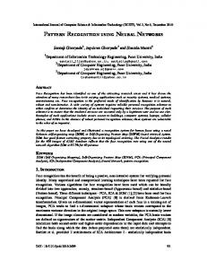
Fig. 2. Theoretical Model Reference controller.
We consider the class of models whose MR controller exists and is stable, in the state domain of interest. The MR controller is well known in the linear literature [11]. C. Theoretical Inverse Model The theoretical inverse of model (2) is defined, if it exists, as the controller which, when cascaded with model (2), imposes the behavior of a pure delay d: y(k+d) = r(k) = yr(k+d) (8) The inverse model is thus the MR controller for E = H = 1 (i.e. the reference model is the delay d). It is known in the linear literature as the “one-step-ahead controller” [11]. D. Design of the Neural Reference Model Controller As will be shown in section IV, only the case of a model without delay (d=1) needs to be considered. The objective is to impose the desired dynamic behavior given by the reference model, i.e. relationship (7), from time k+1 on. Relationship (7) can be rewritten as: y(k+1) = H r(k) + 1 – E y(k+1) (9) Using the model expression (2) with d=1, it follows that: k ϕ y{kk-n+1 , u{k-m+1 = H r(k) + 1 – E y(k+1) (10) We suppose that it is possible to express u(k) as a function g of H r(k) + 1 – E y(k+1), i.e. of the past outputs y{kk-n+1 and inputs u{k-1 k-m+1, such that (10) is verified in the domain of interest. The theoretical MR controller can be expressed as: k k-1 u(k) = g H r(k) + 1 – E y(k+1), y{k-n+1 , u{k-m+1 (11) The MR controller is of order m–1≥0. Using the same derivation, the theoretical inverse model is given by: u(k) = g y r(k+1), y {kk-n+1, u{k-1 (12) k-m+1 The MR controller is thus equivalent to the inverse model driven by the output of a feedforward system defined by the polynomials E and H of the reference model; this output yral(k+1) computed at time k is given by: yral(k+1) = H r(k) + 1 – E y(k+1) (13) This feedforward model is called a rallying model. The equivalence is illustrated in Fig. 3: r
B. Theoretical Model Reference Controller
y
Theoretical MR Controller (E, H, d=1)
u
Model (d=1)
y
⇔
The theoretical MR controller of model (2) is defined, if it exists, as the controller which, when cascaded with model (2) in a simple feedback system, imposes the reference dynamic behavior (4), as shown in Fig. 2: E y(k) = q -d H r(k) (7) Thus, whatever the state of the model at time k, the theoretical MR control input u(k) is such that the behavior of the system {MR controller+model} is identical to the
Reference Model (E, H, d)
r
y
Theoretical MR Controller (E, H, d=1) y ral Rallying Theoretical Model Inverse Model (E, H, d=1) y
u
Model (d=1)
y
Fig. 3. Model Reference controller equivalence for a model without delay.
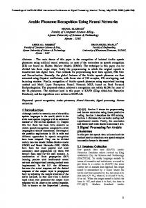
Thus, in order to obtain the MR controller, it is only necessary to estimate the function g, i.e. to train the inverse model. The training system of the inverse of a model without delay is shown in Fig. 4. It consists of: – the reference model generating the desired output sequence; at time k, it computes: y r(k+1) = H r(k) + 1 – E y r(k+1) (14) – the neural inverse model (to be trained); at time k, it computes: k k-1 u(k) = γ yr(k+1), y{k-n+1 , u{k-m+1 ;θ (15) where γ is a nonlinear function implemented by a feedforward network with weights θ. – the model, whose weights are fixed; at time k, u(k) being available, it computes: k y(k+1) = ϕ y{kk-n+1 , u{k-m+1 (16) r
Reference Model (E, H, d=1)
yr
y Neural Inverse Model (to be trained) yr
Back-Prop
u
Model (d=1, fixed) Back-Prop
y
yr + – e
Fig. 4. Training system of the inverse of a nonlinear model without delay.
If the family of functions defined by the feedforward part of the network is rich enough with respect to the complexity of g, and if the training algorithm is efficient, then the function γ implemented by the neural network will be arbitrarily close to the function g in the domain defined by the training sequences. The MR controller is then obtained from the trained inverse model by replacing yr(k+1) in (15) by the output of the rallying model H r(k) + 1 – E y(k+1) : k k-1 u(k) = γ H r(k) + 1 – E y(k+1), y{k-n+1 , u{k-m+1 (17) whose weights θ are now fixed. An advantage of the proposed design of a MR controller is that, if the behavior of the control system based on the MR controller is not entirely satisfactory, it is possible to tune the rallying model without training the MR controller anew. Note that the design of the MR controller is more complex for a model with delay. If d>1, a difference arises from the fact that 1 – E y (k+d) in (10) contains not only past or present outputs, but also the future outputs y(k+1), … y(k+d-1). In that case, the MR controller must be designed and trained as a function of the reference model and of its delay (see [12] for a full treatment of the case d>1). IV. THE INTERNAL MODEL CONTROL SYSTEM In order to show the simplicity of the design of IM control systems, the classic Simple Feedback control system design is first dealt with. Simple Feedback Control System Having trained a MR controller, the design of a Simple Feedback control system is straightforward: the MR
controller is cascaded with the process. In the particular case of a model without delay, the MR controller consists of the inverse model cascaded with the rallying model associated to the reference model, as shown in Fig. 5. The expression of the control is obtained by replacing y by y p in (17): k-1 u(k) = γ H r(k) + 1 – E yp(k+1), yp{kk-n+1, u{k-m+1 (18) k-1 = γ yral(k+1), yp{kk-n+1, u{k-m+1 where yral(k+1) is the output of the rallying model. Neural MR Controller (d=1) y ral Rallying Neural Model Inverse (E, H, d=1) Model yp
r yp
u
yp
Process
Fig. 5. Simple Feedback control system of a process without delay.
As already mentionned in section I, such a control system is intrinsically not robust towards a model mismatch and disturbances, which lead to important steady-state errors. Internal Model Control System The controller must now control the IM. Let us show that the case of a model with delay is dealt with very simply. Model (2) is used as IM; let it be split into: – the delay-deprived model (3): k z(k+1) = ϕ z{kk-n+1, u{k-m+d – a delay (d–1): y(k+d) = z(k+1). What is needed is the MR controller for the delay-deprived model: since the latter is a model without delay, it can be built from: – the inverse of the delay-deprived model; – a rallying model for the delay-deprived model, which is thus defined by the polynomials E and H of the reference model, but with delay d’=1. Its input are the IM setpoint, and the past outputs of the delay-deprived model. The overall IM control system is shown in Fig. 6. r + – eIM
MR Controller of the Delay-Deprived Model zral Rallying Neural Inverse Model of the Delay(E, H, d'=1) Deprived Model z z
r*
u
yp
Process
Internal Model u
DelayDeprived Model
z
yp +
q-(d-1)
y
– eIM
Fig. 6. Internal Model control system of a process with delay.
When u(k-1) becomes available, z(k) is computed by the delay-deprived model : k-1 z(k) = ϕ z{k-1 k-n, u{k-m+d-1 Then, let us consider the computations performed at time k, which is defined as the instant when yp(k) is available: a) the difference between the outputs of the process and of the IM: eIM(k) = y p(k) – y (k) b) the corrected setpoint for the IM: r*(k) = r(k) – eIM(k) c) the output of the rallying model: zral(k+1) = H r*(k) + 1 – E z(k+1) (19) d) the control value, output of the inverse of the delaydeprived model: k k-1 u(k) = γ zral(k+1), z{k-n+1 , u{k-m+d (20) Properties of the proposed IM control system The proposed control system has the basic properties described in section I:
– If the inverse is exact, the output of the delay-deprived model is equal to the output of the rallying model: z(k+1) = H r*(k) + 1 – E z(k+1) If the IM is perfect, the dynamic behavior of the control system is thus identical to the reference behavior in the absence of disturbances. – If only the inverse model is exact, and if the overall control system is stable, the effect of constant disturbances and of a model mismatch are cancelled in the steady-state, which is an important advantage over a Simple Feedback control system. – The rallying model of the MR controller plays the role of the IM filter in the classical IM control system [4] which ensures the robustness of the stability of the control system with respect to a process mismatch, and the smoothness of the control. With our method, the design of the filter is straightforward. Design precautions Let us now specify the design precautions that must be taken in the case of a neural network based IM control system in order to maximize its robustness properties. One must be aware that the validity domain of the neural inverse model is restricted to the region of the state space it was trained in. This training region must be larger than the operating region desired for the process since, during the operating phase, the neural inverse model controls the IM, which might evolve in a larger region of the state space than the process, due to a model mismatch and to disturbances. Remarks Neural IM control system are often simplified in the two following ways: – Instead of the feedforward rallying model, the feedback reference model with input r* and output zr* is used to drive the inverse model, as in [7] for example. This assumes that z(k) = zral(k) ∀k holds, i.e. that the inverse model is exact. But, dealing with general nonlinear neural models, this is usually not true. As a matter of fact, we showed in [13] that an IM control system with a rallying model is more robust towards a controller/model mismatch than with the reference model. – The IM is removed, in [6] for example, as in Fig. 7: r
r* + – eIM
Reference Model (E, H, d'=1)
zr *
Neural Inverse of the DelayDeprived Model
u
Process
q -d
systems are designed for these processes, and compared to Simple Feedback control systems on representative setpoint sequences, in the presence of disturbances. A. Process ‘1’ (without delay) Process ‘1’ is simulated by: yp(k+1) = h yp(k), yp(k-1), u(k) 2 (21) 24+yp(k) = yp(k) – 0.8 u(k) 2 yp(k-1) + 0.5 u(k) 30 1+u(k) Analysis of the Process Behavior For large input amplitudes, the process is a stable nonlinear oscillatory low-pass filter (see Fig. 8). More specifically, around operating points {y 0 , u0 }, its behavior is the following: (i) around {0, 0}, it behaves like a damped first-order filter with time constant 3.6 T (T is the sampling period); (ii) around operating points corresponding to 0.1 < |u 0 | < 0.5, it behaves like an oscillatory second-order filter with pseudo-period 5 T; (iii) for operating points corresponding to larger u0 , the behavior becomes more complex. The amplitude of u is limited to [-5; 5] by a saturation of the actuator output; for a constant amplitude 5 of the control input, the output is equal to 2.7, and for an amplitude of -5, to -2.3. Reference Model The reference regulation and tracking dynamic behavior is chosen to be given by a damped linear second-order filter with time constants T and 1.2 T, and with unit static gain: yr(k+1) + e1 yr(k) + e2 yr(k-1) = h0 r(k) + h1 r(k-1) (22) where: e1 = –0.803; e2 = 0.160; h0 = 0.232; h1 = 0.126. 1) Modeling of the Process The training control input sequence consists of pulses of random amplitude in the range [-5; 5] with a duration of 10 sampling periods; the total length of the sequence is 1000. The control input sequence used for the performance estimation is generated in the same manner, and is shown in Fig. 8. u
5
0
yp yp + yr* –
-5
yp 0
200
400
600
800
1000
Fig. 8. Performance estimation sequences for modeling. eIM
Fig. 7. Simplified Internal Model control system to avoid.
As a matter of fact, the process is usually equipped with an actuator whose output is limited in amplitude. The existence of an inverse is then restricted to these limits, and so the legimity of the IM removal. As a consequence, the control system of Fig. 7 is not immune to wind-up (the loop with the delay d creates an integrator that is never switched off). V. ILLUSTRATIVE EXAMPLES
We retained the following candidate: y(k+1) = ϕ y(k), y(k-1), u(k) (23) where ϕ is a function implemented by a fully connected network1 with 5 sigmoidal hidden neurons and a linear output neuron. Using a quasi-Newton algorithm, a “training mean square error” (TMSE) of 1.2 10-5 and a 1 A fully connected network with Ne inputs x 1 , …, xN e , and Nn ordered neurons, is such that the output xi of neuron i is given by: i-1
x i = fi
∑ θij x j
i = Ne+1 to Ne+Nn
j=1
This section presents the modeling and control of two simulated processes, without and with delay. IM control
where f i is the activation function of neuron i. Neuron Ne+Nn is the output neuron.
“performance mean square error”, i.e. a MSE on the sequences for performance estimation (PMSE), of 1.4 10 -5 were obtained. 2) Training of the Inverse Model We assume that the process is to be controlled for setpoint pulses of amplitude in the range [-2; 2.5]. The inverse of model (23) is trained using the training system described in section III.D Fig. 4; it consists of: – the reference model (22) generating the desired output sequence yr(k) from the setpoint sequence r(k) . – the neural inverse model (to be trained): u(k) = γ yr(k+1), y(k), y(k-1); θ (24) where γ is a function implemented by a fully connected network with sigmoidal hidden neurons and where the activation function of the output neuron is the saturation function between [-5; 5] (which corresponds to the actuator limits). – the neural model (23), whose weights are now fixed. The training setpoint sequence {r(k)}consists of pulses of random amplitude in the range [-2.5; 3] with a duration of 20 sampling periods; the total length of the sequence is 1000. The maximum amplitudes are chosen so as to fully explore the desired output amplitude range [-2; 2.5] and to encounter the saturations. With 5 hidden neurons, a TMSE of 5.6 10 -4 is obtained. Since most errors are due to the control saturation, adding neurons does not improve the TMSE significantly. 3) Control of the Process The process is affected by a randomly occuring pulseshaped disturbance of amplitude 0.5, denoted by da, acting additively on the output: x p(k+1) = h x p(k), x p(k-1), u(k) (25) y p(k) = x p(k) + da(k) The setpoint sequence consists of pulses with amplitudes in the range [-2; 2.5]. The Simple Feedback control system is first tested. Simple Feedback Control System The behavior of the Simple Feedback control system is shown in Fig. 9:
disturbance occurs, there is a small steady-state error, due to a controller inaccuracy. As a matter of fact, the value of the output of the model reaches 3, that is the limit of the domain the controller was trained in. Retraining the controller in a larger domain leads to zero error, but our goal was to emphasize the importance of the design precautions sketched in section IV. 5
0
-5 0
50
100
150
200
250
300
Fig. 10. Internal Model control of process ‘1’ (thin line: r; dotted line: da ; dashed line: u; thick line: yp ; thick dotted line: y).
B. Process ‘10’ (with delay) In order to show the similarity of the design in the case of a process with delay, the second process is chosen to be characterized by the same input-output relationship than process ‘1’, but with a delay d=10. Process ‘10’ is thus simulated by the following discrete-time system: x p(k+1) = h x p(k), x p(k-1), u(k-9) (26) y p(k) = x p(k) + da(k) We choose to deduce a model of (26) from the model of process ‘1’ (23) by adding a delay of 9 time steps to it: y(k+1) = ϕ y(k), y(k-1), u(k-9) (27) As shown in section IV for models with delay, the neural controller (24) can be used in the IM control system for process ‘10’ (but not in a Simple Feedback control system, we will therefore not make the comparison for this process). Its behavior is shown in Fig. 11: 5
0
5 -5 0
50
100
150
200
250
300
Fig. 11. Internal Model control of process ‘10’ (thin line: r; dotted line: da; dashed line: u; thick line: yp ; thick dotted line: z).
0
-5 0
50
100
150
200
250
300
Fig. 9. Simple Feedback control of process ‘1’ (thin line: r ; dotted line: da; dashed line: u; thick line: yp ).
A disadvantage of Simple Feedback control appears clearly: constant disturbances lead to important steadystate errors. Internal Model Control System The behavior of the IM control system is shown in Fig. 10. y denotes the output of the IM. Thanks to the IM control structure, the performance in the steady-state is greatly improved (it appears clearly in the control error shown in Fig. 12). Nevertheless, the second time the
z denotes the output of model (27) deprived from its delay. If we except the uncancellable errors due to the pure delay, the performance of the control system of process ‘10’ is almost identical to that of process ‘1’. 1
0
-1
0
50
100
150
200
250
300
Fig. 12. Comparison of the control errors (thin dashed line: da; thin continuous line: Simple Feedback control of process ‘1’; thick dotted line: Internal Model control of process ‘1’; thick line: Internal Model control of process ‘10’).
The errors of the three control systems are shown in Fig. 12. The control error is computed as the difference between the output of the reference model (not shown on the graphs for the sake of clarity) and of the process. VI. CONCLUSION We have presented a design procedure of Internal Model control systems for the problem of tracking a setpoint sequence with the dynamic behavior given by a reference model. We have shown that the design of the Model Reference controller can be performed independantly from the delay of the process, since it can be built of the inverse of the model deprived from its delay (trained), and of a rallying model associated to the reference model. Moreover, the control system using the Model Reference controller can be modified by tuning the rallying model (not trained), if necessary. The advantage of Internal Model control systems is their robustness with respect to a model mismatch and to disturbances. Nevertheless, these properties are only obtained if the Model Reference controller is close to the theoretical one; we have thus stressed the design precautions that must be taken in order to avoid the consequences of a possible controller/model mismatch. The proposed Internal Model design procedure was successfully applied to the piloting (velocity control) of a 4WD Mercedes vehicle [14]. We are now investigating the use of affine black-box models, which allow a direct and thus exact design of their inverse model [12]. VII. REFERENCES [1] Sanner R., Slotine J.-J., “Stable adaptive control of robot manipulators using ‘neural’ networks”, Neural Computation Vol. 7 N°4, 1995, pp. 753-790. [2] Narendra K. S., Mukhopadhyay S., “Adaptive control of nonlinear multivariable systems using neural networks”, Neural Networks Vol. 7 N°5, 1994, pp. 737-752. [3] Morari M., Zafiriou E., Robust process control, Prentice-Hall International Editions, 1989. [4] Economou G. C., Morari M., Palsson B. O., “Internal Model control. 5. Extension to nonlinear systems”, Ind. Eng. Chem. Process Des. Dev. Vol. 25, 1986, pp. 403-411. [5] Alvarez J., “An internal model controller for nonlinear systems”, Proceedings of the 3rd European Control Conference, Rome, Italy, September 1995, pp. 301-306. [6] Psichogios D. C., Ungar L. H., “Direct and indirect model based control using artificial networks”, Ind. Eng. Chem. Res. Vol. 30 N°12, 1991, pp. 2564-2573. [7] Hunt K., Sbarbaro D. “Neural networks for nonlinear internal model control”, IEE Proc.-D Vol. 138 N°5, 1991, pp.431-438. [8] Rivals I., Personnaz L., “Black-box modeling with state-space neural networks”, to appear in Neural Adaptive Control Technology I, R. Zbikowski and K. J. Hunt eds., World Scientific, 1996. [9] Nerrand O., Roussel-Ragot P., Personnaz L., Dreyfus G., “Neural networks and nonlinear adaptive filtering:
unifying concepts and new algorithms”, Neural Computation Vol. 5 N°2, 1993, pp. 165-199. [10] Rivals I., Personnaz L., Dreyfus G., Canas D., “Realtime control of an autonomous vehicle: a neural network approach to the path following problem”, 5th International Conference on Neural Networks and their Applications, Nîmes, France, 1993, pp. 219-229. [11] Goodwin G. C., Sin K. S., Adaptive filtering prediction and control, Prentice-Hall, New Jersey, 1984. [12] Rivals I., Personnaz L., “Model Reference control using neural networks”, 1996, submitted for publication. [13] Rivals I., Modélisation et commande de processus par réseaux de neurones ; application au pilotage d’un véhicule autonome, Thèse de Doctorat de l’Université Paris 6, 1995. [14] Rivals I., Canas D., Personnaz L., Dreyfus G., “Modeling and control of mobile robots and intelligent vehicles by neural networks”, IEEE Conference on Intelligent Vehicles, Paris, 24-26 octobre 1994, pp. 137-142.