Intraseasonal variability in barrier layer ... - Wiley Online Library

JOURNAL OF GEOPHYSICAL RESEARCH, VOL. 116, C03009, doi:10.1029/2010JC006657, 2011

Intraseasonal variability in barrier layer thickness in the south central Bay of Bengal M. S. Girishkumar,1 M. Ravichandran,1 M. J. McPhaden,2 and R. R. Rao3 Received 16 September 2010; revised 27 November 2010; accepted 16 December 2010; published 5 March 2011.

[1] Time series measurements of temperature and salinity recorded at 8°N, 90°E in the south central Bay of Bengal from a Research Moored Array for African‐Asian‐Australian Monsoon Analysis and Prediction buoy, along with satellite altimetry and scatterometer data, are utilized to describe the seasonal and intraseasonal variability of barrier layer thickness (BLT) during November 2006 to April 2009. The BLT shows strong seasonality with climatological minima during both March–May and August–September and maxima during December–February. Large‐amplitude, intraseasonal fluctuations in BLT are observed during September 2007 to May 2008 and during September 2008 to April 2009. The observed intraseasonal variability in BLT is mainly controlled by the vertical movement of isothermal layer depth (ILD) in the presence of a shallow mixed layer. Further, the analysis shows that both ILD and BLT are modulated by vertical stretching of the upper water column associated with westward propagating intraseasonal Rossby waves in the southern bay. These waves are remotely forced by intraseasonal surface winds in the equatorial Indian Ocean. Citation: Girishkumar, M. S., M. Ravichandran, M. J. McPhaden, and R. R. Rao (2011), Intraseasonal variability in barrier layer thickness in the south central Bay of Bengal, J. Geophys. Res., 116, C03009, doi:10.1029/2010JC006657.

1. Introduction [2] The Bay of Bengal is a unique semienclosed tropical basin, forced locally by the semiannually reversing monsoon winds and remotely by zonal winds in the equatorial Indian Ocean (EIO) [McCreary et al., 1993]. In addition, the Bay of Bengal (referred to hereafter as the bay) also receives large quantity of freshwater by excess precipitation and river runoff over evaporation [Varkey et al., 1996; Rao and Sivakumar, 2003]. This large freshwater flux into the bay makes the waters in the near‐surface layer less saline and maintains strong haline stratification [Shetye et al., 1996]. This leads to the formation of an intermediate “barrier layer” (BL), the layer between the base of the mixed layer and the top of the thermocline [Lukas and Lindstrom, 1991; Vinayachandran et al., 2002; Rao and Sivakumar, 2003; Thadathil et al., 2007]. [3] The BL acts as a barrier to turbulent entrainment of cooler thermocline waters into mixed layer and thereby plays an important role on ocean surface layer heat budget and sea surface temperature (SST) [Lukas and Lindstrom, 1991]. In addition, the BL may induce inversions in the

1 Indian National Centre for Ocean Information Services, Ministry of Earth Sciences, Hyderabad, India. 2 NOAA Pacific Marine Environmental Laboratory, Seattle, Washington, USA. 3 Department of Meteorology and Oceanography, Andhra University, Visakhapatnam, India.

Copyright 2011 by the American Geophysical Union. 0148‐0227/11/2010JC006657

vertical temperature profile by trapping a significant part of the penetrating solar radiation [Anderson et al., 1996]. In the bay, thermal inversions supported by BLs play a significant role in warming the mixed layer during the winter monsoon by entrainment of warm subsurface water [de Boyer Montégut et al., 2007b]. [4] The signature of intraseasonal variations has been observed in the bay for SST [Sengupta and Ravichandran, 2001; Vecchi and Harrison, 2002; Rao et al., 2006] and for ocean currents [Durand et al., 2009]. A better understanding of this intraseasonal variability may be valuable for short‐ term climate forecasting in the tropics. Earlier studies showed that intraseasonal variability of SST in the bay could be an important factor in the evolution of active and break cycles of the summer monsoon [Vecchi and Harrison, 2002]. The halocline in the surface layer has the potential to maintain the warm SST (>28°C) in the bay [Shenoi et al., 2002], and hence plays a crucial role in monsoon precipitation over the ocean and the surrounding land. Sengupta et al. [2007] showed that the existence of BLs reduces the effects of storm induced cooling in the mixed layer, and hence favors the intensification of tropical cyclones during the postmonsoon season (October–November) in the bay. [5] The BL also inhibits transfer of nutrients into the euphotic zone from below, and leads to low biological productivity in the bay, particularly during the summer monsoon season [Prasanna Kumar et al., 2002]. Weakening of the BL can also enhance primary productivity by allowing greater injection of nutrients into the mixed layer [Girishkumar et al., 2010]. Rao et al. [2002] have shown that near‐surface stratification in the bay prevents Indian Ocean Dipole (IOD)

C03009

1 of 9

C03009

GIRISHKUMAR ET AL.: BARRIER LAYER IN THE BAY OF BENGAL

related upwelling from influencing SST. Thus the above studies emphasize the importance of understanding the evolution of BL to elucidate air‐sea interaction processes and ocean primary productivity in the bay. [6] Investigations of the seasonal evolution of the BL in the bay using monthly temperature and salinity climatologies derived from historical observations conclude that the BL is most prominent in February [Sprintall and Tomczak, 1992; Rao and Sivakumar, 2003]. de Boyer Montégut et al. [2007a] and Mignot et al. [2007] also reported that barrier layer thickness (BLT) is maximum during winter in the bay. Thadathil et al. [2007] have made a detailed study of seasonal variability of the BL and its formation mechanisms in the bay. They reported that during both the summer and winter monsoon seasons the surface circulation and the redistribution of low saline waters show a dominant influence on the observed BLT distribution. Also, Ekman pumping and propagating Rossby waves forced by Kelvin waves propagating along the eastern boundary contribute significantly in modulating variability in BLT on seasonal time scales. [7] Using in situ observations made from a stationary location in the northern bay (20°N, 89°E) during August– September 1990, Murty et al. [1996] reported that the thickness of the mixed layer based on temperature is always greater than that based on density implying the presence of a significant BL. Vinayachandran et al. [2002] studied the formation of BL in the bay during the summer monsoon and its intraseasonal variability using the hydrographic observations made in the northern bay (18.5°N, 89°E) from 27 July to 6 August 1999, and reported that the BL was about 25– 30 m thick. They further showed that a decrease in mixed layer depth (MLD) due to the arrival of fresh water plumes from river discharge and rainfall leads to the formation BLs. Due to lack of systematic measurements of temperature and salinity with high temporal resolution, most of these studies focused mainly on the seasonal time scale and short period intraseasonal variations using limited data sets. Hence, much less is known about intraseasonal variability of the BL and how that variability changes from year to year in the bay. [8] The main aim of the present work is to describe and explain the observed intraseasonal variability of BLT at 8°N, 90°E in the south central bay during 2006–2009 and the role that intraseasonal planetary waves play in modulating that variability. We have chosen this site because of its long record length (approximately 2.5 years) and its location in a region of significant mean BLT. Our interest in wave influences on BLT changes is motivated by modeling and observational studies that have shown winds over the EIO, and alongshore winds in the eastern bay play an important role in modulating the circulation features in the bay on seasonal time scales [Potemra et al., 1991; Yu et al., 1991; McCreary et al., 1993, 1996; Yang et al., 1998; Shankar et al., 2002; Yu, 2003; Kantha et al., 2008]. Westerly (easterly) winds in the central and eastern EIO force downwelling (upwelling) first and second baroclinic mode Kelvin waves that propagate eastward along the equator then traverse the rim of the bay as coastal Kelvin waves [Potemra et al., 1991]. McCreary et al. [1993] and Yang et al. [1998] have further shown that meridional winds along the eastern rim of the bay also trigger coastal Kelvin waves. Recent studies [Iskandar et al., 2005; Han, 2005; Fu, 2007; Vialard et al., 2009; Oliver and Thompson, 2010] have revealed the existence of intraseasonal

C03009

(30–90 days) baroclinic mode Kelvin waves in the eastern EIO, which are forced primarily by intraseasonal wind variability (30–90 days). When these waves propagate as coastal Kelvin waves into the eastern bay, they then radiate westward as low baroclinic mode Rossby waves into the interior [Potemra et al., 1991; Yu, 2003; Rao et al., 2010]. Bosc et al. [2009] noted that BLT can change from relative deepening or shoaling of the isothermal layer depth (ILD) and MLD due to dynamical processes such as westward propagating planetary waves. Yu [2003] and Rao et al. [2010] further suggest that on seasonal time scales remote forcing from the EIO controls the large variability of upward/downward thermocline movements. However, the influence of these intraseasonal waves on BLT in the bay is not yet reported so far. [9] The paper is organized as follows. Section 2 describes the data sets utilized and the methodology followed. The observed BLT variability at the buoy location is described in section 3. The causative mechanisms for the observed variability in BLT are examined in section 4, and the main conclusions are summarized in section 5.

2. Data and Methodology [10] The Research Moored Array for African‐Asian‐ Australian Monsoon Analysis and Prediction (RAMA) [McPhaden et al., 2009] is the moored buoy component of the Indian Ocean Observing System (IndOOS), which consists of a variety of satellite and in situ measurement systems [Meyers and Boscolo, 2006]. Daily time series of temperature and salinity are obtained from the RAMA buoy in the south central bay (8°N, 90°E, red square in Figure 1). These data provide a unique time series data set to examine the evolution of near‐surface thermal and salinity structure and to describe the observed intraseasonal variability of BLT in this region. Satellite measurements are also used to study the dynamic and thermodynamic processes that are important for BLT variability at the buoy location. [11] Data are available from the RAMA buoy during 1 November 2006 to 30 April 2009. The time series of temperature and salinity are continuously measured at depths of 1, 10, 13, 20, 40, 60, 80, 100, 120, 140, 180, 300, and 500 m and 1, 10, 20, 40, 60, 100, and 120 m respectively. We consider measurements at 1 m nominally as from the surface. [12] We will mainly focus on analyzing data in the upper 100 m. The data are linearly interpolated in the vertical to 1 m intervals to facilitate analysis. To understand how accurately BLT can be estimated from these buoy data, which have fairly coarse vertical resolution, we have picked about 25 profiles from a nearby Iridium Argo float that has typically 2 m vertical resolution (i.e., higher vertical resolution than the typical 10 m resolution in the upper 200 m for most Argo floats). This float was typically within 1.5° of the buoy location. Parameters such as MLD, ILD, and BLT were computed from these data and compared to the same quantities estimated from Argo data sampled at RAMA buoy depths. Differences between these estimates provide an idea about the accuracy of these parameters derived from RAMA buoy. The root‐mean‐square difference for MLD, ILD, and BLT are 3.5, 5.0, and 4.6 m, respectively. These differences are generally small relative to the amplitude of the variations we observed in the bay, so the above analysis indicates that

2 of 9

C03009


C03009

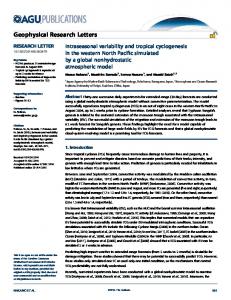
Figure 1. (a) Observed time series of surface wind vectors (m s−1) at 4 m height, (b) depth‐time section of temperature (°C), (c) depth‐time section of salinity, and (d) barrier layer thickness (m) derived from the temperature and salinity climatology (WOA05, red line) and derived from RAMA buoy measurements (black line) at 8°N, 90°E in the Bay of Bengal during November 2006 to April 2009. In Figures 1b and 1c, the thick, dashed, and thin lines indicate MLD (m), ILD (m), and depth of the 23°C isotherm (m), respectively. The red square in the inset map represents the buoy location.

RAMA buoy measurements provide reasonable estimates of these quantities despite their relatively coarse vertical resolution. [13] A Triangle Trans Ocean Buoy Network (TRITON) mooring deployed by the Japan Agency for Marine Earth Science and Technology (JAMSTEC) at 1.5°S and 90°E is used to compute the depth of the 23°C isotherm, which is a measure of the thermocline depth. TRITON moorings are very similar to ATLAS moorings in their vertical and temperature sampling schemes. These data is utilized to understand the relationship of D23 to surface zonal winds and sea surface height anomaly (SSHA) in the EIO. [14] A satellite gridded SSHA product [AVISO Altimetry, 2009] was utilized to characterize the nature of propagating Rossby waves. QuikSCAT [Wentz et al., 2001] wind data are utilized to characterize the wind variability over the equator and along the southeastern rim of the bay. The sources, resolutions, and the accuracies of the data sets utilized in this study are shown in Table 1.

[15] The MLD and ILD are defined following Sprintall and Tomczak [1992] and Rao and Sivakumar [2003]. The ILD is defined as the depth where the temperature is 0.8°C less than SST [Kara et al., 2000; Du et al., 2005]. The MLD is calculated as the depth where the density is equal to the sea surface density plus the increment in density equivalent to 0.8°C. This increment of the density is determined by the coefficient of thermal expansion, which is calculated as a function of SST and sea surface salinity. The BLT is defined as the difference of ILD and MLD. A Butterworth band‐ pass filter is used to extract intraseasonal (40–100 day) signals [Emery and Thomson, 1998] in zonal wind speed, SSHA, ILD, MLD, and BLT.

3. Observed Wind Speed, Temperature, Salinity, and BLT at the Buoy Location [16] The observed temporal evolution (without bandpass filtering) of wind speed, temperature and salinity at the buoy

3 of 9

C03009


C03009

Table 1. Source, Temporal and Spatial Resolution, and Accuracy of Data Set Used in This Study Parameter

Source

Temporal and Spatial Resolution

Accuracy

AVISO blended sea surface height anomaly QuikSCAT wind data RAMA temperature data

http://www.aviso.oceanobs.com

0.33°, 7 day composites

2.5–4 cm

http://www.ssmi.com http://www.pmel.noaa.gov/tao

0.25°, daily 1, 10, 13, 20, 40, 60, 80, and 100 m depth, daily 1, 10, 20, 40, 60, and 100 m depth, daily 1.5, 25, 50, 75, 100, 125, 150, 200, 250, 300, 500, and 750 m depth

2 ms−1 and ±20° ±0.003°C and ±0.05°C

RAMA salinity data TRITON temperature data

http://www.pmel.noaa.gov/tao http://www.jamstec.go.jp/jamstec/TRITON

location is shown in Figure 1. The wind speed shows a strong annual cycle with southwesterly during May to October and northeasterly during November to April. The depth‐time section of temperature (Figure 1b) at the buoy location shows a semiannual seasonal cycle with two warm seasons during April–May and October–November, and two cool seasons during December–February and June–September. The warm near‐surface layer during spring penetrates down to 40–50 m. The temporal evolution of temperature (Figure 1b) shows a strong temperature gradient around the 23°C isotherm. The average position of this isotherm is around 100 m depth and it exhibits significant upward and downward movements on intraseaonal time scales. [17] The temporal evolution of near‐surface salinity (Figure 1c) shows relatively low saline waters in the near‐ surface layers compared to subsurface layers. The evolution of near surface salinity variability at the buoy location (Figure 1c) shows the existence of low saline water ranging from 32.2 to 34.6 in the upper 30 to 40 m. The existence of low saline waters near the surface and high saline waters below 30 m depth leads to a strong halocline in the near‐surface layer leading to a shallow salinity‐dependent mixed layer and to formation of a barrier layer below it. The BLT derived from the temperature and salinity climatology of Locarnini et al. [2006] at the buoy location and from the RAMA buoy is shown in Figure 1d. The BL climatology shows minimum thickness during March–May and August–September, and a maximum thickness during December–February. Daily evolution of BLT from the RAMA data shows strong seasonality, wherein BLT builds up from August (20–25 m) and reaches maximum thickness during the winter (60–75 m) and decrease afterward in spring (20 m). Large warming in the near surface layer due to intense solar heating during spring shoals the ILD even in the presence of a halocline [Thadathil et al., 2007]. This is one of the reasons for minimum BLT during the spring as shown in Figure 1d. The BLT is at minimum during winter 2006–2007, January 2008, summer 2008, and March 2009. However, during the winter of 2006–2007, the BLT is very weak compared to winters of 2007–2008 and 2007–2009. In addition, large amplitude intraseasonal variability is observed in BLT, which is particularly pronounced during September 2007 to May 2008 and September 2008 to April 2009.

4. Forcing Mechanisms for BLT Variability 4.1. Evolution of MLD and ILD at the Buoy Location [18] Earlier several studies show that the primary mechanism for the development of the seasonal BL in the bay is

±0.02 ±0.002°C

the formation of shallow salinity driven mixed layer due to freshening in the surface layer [Thadathil et al., 2007]. That freshening is the result of intense precipitation and the redistribution low saline river discharge by the horizontal circulation [Rao and Sivakumar, 2003; Jensen, 2003; Sengupta et al., 2006; Parampil et al., 2010]. Processes that can cause a deepening/shoaling of mixed layer are surface cooling/ warming by air‐sea fluxes of heat, fresh water fluxes, turbulent transfer of momentum from wind, and horizontal current convergence and divergence. Wind‐induced mixing and convective overturn due to net heat loss from sea surface increases turbulent entrainment at the bottom of the mixed layer and can lead to deepening of the mixed layer and a thinning of the BL. Positive fresh water and heat flux, both of which contribute to a positive buoyancy flux, stabilize the surface layer and can cause the mixed layer to shoal. [19] To understand the relative influence of MLD and ILD on BLT variability at the buoy location, we have calculated the correlation between changes in BLT and ILD and between BLT and MLD. The correlations of unfiltered BLT with MLD and unfiltered BLT with ILD for the entire period of observation are −0.39 and 0.45, respectively. After band‐ pass filtering, the correlation of BLT with MLD is −0.33 and BLT with ILD is 0.67. Focusing on just those periods of pronounced intraseasonal variability in BLT (September 2007 to May 2008 and September 2008 to April 2009), the corresponding correlations between band‐pass filtered BLT with MLD is −0.35 and between BLT with ILD is much higher at 0.83. All correlations are statically significant at 95% confidence level. This analysis indicates that thickening of the BL is largely due to deepening of the ILD and secondarily to shoaling of the MLD. Note that though intraseasonal variability in ILD is seen during the winter 2006–2007 (Figure 2), the corresponding amplitude of intraseasonal variability of BLT is not significant then since the ML is also varying in association with the relatively strong winds (Figures 1a and 1b). [20] Yu [2003] suggested that on seasonal time scales the upward/downward movement of the thermocline in the bay is controlled by Ekman pumping and/or remote forcing from the EIO. In the Ekman pumping process, cyclonic (anticyclonic) wind stress curl causes divergence (convergence) of the local Ekman currents that in turn, induces upwelling (downwelling) beneath the Ekman layer, thereby affecting the ILD [Gill, 1982]. In order understand the relative contribution of Ekman pumping to the variability of ILD, daily Ekman pumping velocity (WEP, m d−1) was calculated using the expression of Yu [2003] from QuikSCAT wind data with

4 of 9

C03009


C03009

Figure 2. Daily evolution of Ekman pumping velocity (m d−1, blue line) and rate of change of ILD (∂h/∂t in m d−1, red line) at the buoy location. 0.25 degree spatial resolution. The local rate of change of ILD (∂h/∂t) was also estimated from the buoy data (Figure 2). The rate of change of ILD shows strong intraseasonal variability, with large magnitude during November to April compared to other seasons. Furthermore, it is apparent that local Ekman pumping plays only a minor role in the modulation of ILD, particularly during the periods of large intraseasonal oscillations. Hence, remote processes must be important in affecting ILD. In order to understand the role of remote forcing from EIO at the buoy location, SSHA data obtained from altimeter data are examined in section 4.2. 4.2. Role of Intraseasonal Rossby Waves [21] The observed time series of D23, ILD and SSHA at the buoy location in the bay and EIO (Figure 3) are utilized to seek a relationship between these variables on the assumption that baroclinic mode wave dynamics are important in governing their evolution. The correlation between D23 and SSHA in the bay is 0.86; similarly the correlation between ILD and SSHA is 0.70. At the buoy location (1.5°S, 90°E), the correlation between SSHA and D23 is 0.75. This correlation analysis (with all correlations statistically significant

at 95% confidence level) shows that SSHA serves as a good proxy to study intraseasonal thermocline variability at the buoy location in the bay. Hence, SSHA is utilized to understand the role of propagating features on intraseasonal variability in ILD. [22] During the study period, winds in EIO show significant intraseasonal variability, with large amplitude during the monsoon transitions (Figure 3b). Westerly (easterly) wind events lead to positive (negative) SSHA and to deeper (shallower) thermocline depths in the eastern EIO with a lag of a few days (Figure 3b). In general, the surface zonal wind stress and SSHA in the EIO have a maximum correlation coefficient of 0.80 when the SSHA lags the surface zonal wind stress by 11 days, in rough agreement with Hase et al. [2008] and Rao et al. [2010]. The estimated phase speed of propagating features in EIO is approximately 2.3 m s−1 in good agreement with phase speed of Kelvin waves as revealed by earlier studies [Iskandar et al., 2005]. Han [2005] and Sengupta et al. [2007] found that westerly wind events on intraseasonal time scales along the equator produce downwelling Kelvin waves that propagate along the equator. When the winds change from westerly to easterly, upwelling

Figure 3. (a) Daily evolution of ILD (m, scale on left side, dashed red line), D23 (m, scale on right side, thin red line), and SSHA (cm, black thick line) at the 8°N, 90°E buoy location. (b) Time series of zonal surface wind stress (N m−2, black line) averaged over the black box bounded by 1°N–1°S, 70°–90°E, SSHA (cm, red dashed line) averaged over the red box bounded by 1°N–1°S, 90°–100°E, and D23 (m, green line) from moored buoy located at 1.5°S and 90°E (green circle) during November 2006 to April 2009. 5 of 9

C03009


Figure 4. (a) Amplitude spectrum based on Fast Fourier Transform [Emery and Thomson, 1998] of zonal wind speed (m s−1) averaged over the black box bounded by 1°N–1°S, 70°–90°E. (b) SSHA (cm) at EIO averaged over the black box bounded by 1°N–1°S, 70°–90°E (black line), SSHA at buoy (red line), and D23 (m) at the 8°N, 90°E buoy location (green line).

C03009

Kelvin waves are generated that propagate eastward along the equator. [23] Power spectra of SSHA and zonal wind in the EIO, and SSHA and D23 at the buoy location in south central bay (Figures 4a and 4b), clearly show dominant peaks in the period band of 40–100 days. After band‐pass filtering the time series in Figures 3a and 3b to emphasize 40–100 day periods, the correlation between D23 and SSHA (ILD and SSHA) is 0.91 (0.76). Similarly the correlation between band‐pass filtered time series of SSHA and D23 at the equator is 0.79 and the correlation between zonal wind stress and SSHA is 0.86 when the SSHA lags the surface zonal wind stress by 11 days. The above analysis indicates the importance of intraseasonal zonal winds along the eastern EIO modulating the corresponding SSHA, thermocline depth, and ILD variability in southern Bay of Bengal consistent with the findings of Vialard et al. [2009]. [24] To understand the role of intraseasonal wind variability in the eastern EIO on the generation of intraseasonal equatorial Kelvin waves and Rossby waves in the southern bay, following the method of Yu [2003] and Kantha et al. [2008], the time‐longitude section of 40–100 day band‐ pass filtered time series of zonal wind along the equator (1°S–1°N), SSHA along the equator to the Sumatra coast, and along the latitude belt 7°N–10°N in the bay are presented in Figures 5a, 5b, and 5c, respectively. The continuous

Figure 5. Time longitude plots of 40–100 day band‐pass filtered (a) zonal wind (m s−1) along the equator, (b) SSHA (cm) at equator and off Sumatra coast, (c) SSHA (cm) along 8°N in the southern Bay of Bengal and (d) time series of ILD (m, not filtered) at the buoy location. (e) time series of 40–100 days band‐pass filtered ILD (m) and SSHA (cm) at the buoy location. (Note the east‐west reversal shown in Figure 5c.) 6 of 9

C03009


Figure 6. Schematic of Rossby wave‐induced upwelling/ downwelling on BLT variability.

propagation of negative (positive) SSHA signals eastward along equator, poleward along the coast of Sumatra and westward along 8°N is clearly seen in the Figures 5b and 5c in response to intraseasonal time scales wind forcing in the eastern EIO. To estimate the speed of these propagating features, we perform a lag correlation analysis. The correlation between 40 and 100 day band‐pass filtered time series of SSHA at 0°, 97°E and 5°N, 95°E shows a maximum value of 0.75 at a lag of 6 days. The estimated phase speed of the Kelvin wave along the coast of Sumatra is therefore approximatelly 2.5 m s−1, which is in good agreement with the intraseasonal first baroclinic mode Kelvin wave speed estimated in EIO [Iskandar et al., 2005]. To estimate the phase speed of the westward propagating signal along 8°N in the southern bay, a lag correlation analysis is performed between 40 and 100 day band‐pass filtered time series of SSHA in the eastern bay (at 8°N, 93°E) and that at the buoy location. A maximum correlation of 0.53 was found at a lag of 16 days, implying a westward phase speed of approximately 0.23 m s−1. The theoretical Rossby wave phase speed at 8°N calculated using the expression given by Jury and Huang [2004] is 0.21 ms−1. The estimated Rossby wave speed thus is in agreement with that expected from theory. This estimate also compares well with earlier results of Yang et al. [1998] and Yu [2003]. [ 25 ] According to linear wave theory [Shankar and Shetye, 1997; Vialard et al., 2009], the theoretical upper bound on allowable periods of the first baroclinic mode Rossby waves at 8°N is 42 days. Coastal Kelvin waves with longer periods will radiate westward as Rossby waves, whereas Kelvin waves at shorter periods will remain trapped to the coast. Hence, intraseasonal Rossby waves at periods of 40–100 days are permissible and in theory can exist at 8°N. The above analysis shows the existence and connectivity of these waves with intraseasonal Kelvin waves along the equator and the coast in the bay. [26] Due to westward propagation of upwelling (downwelling) Rossby waves the thermocline and ILD shoals (deepens) in the bay [Yu, 2003] such that the BL becomes thinner (thicker). The shoaling (deepening) of ILD due to westward propagating upwelling (downwelling) Rossby waves is seen in Figure 5d. The shoaling (deepening) of the ILD leads to thinning (thickening) of the BL (Figure 1b). Thus the observed ILD and BLT variability at the buoy location can be attributed to the westward propagating waves on intraseasonal time scales, particularly during winter. In order to see the intraseasonal variability of ILD and SSHA at the buoy location, 40–100 days band‐pass filtered are

C03009

shown in Figure 5e. It is seen from Figure 5e that the ILD and SSHA are coherent, especially during winter. [27] Figure 6 shows a schematic diagram of how intraseasonal Rossby waves affect the BLT. Even though the BL exists most of the time due to the presence of shallow MLD, intraseasonal variability is modulated by Rossby wave generated variations in ILD. The vertical velocity associated with equatorial waves is zero at surface (assuming a rigid lid approximation) and it would increase roughly linearly with depth near the surface. Thus vertical velocity at the level of the ILD is thus greater than at the level of the MLD. This means that though the BL exists most of the time due to shallow salinity stratification, intraseasonal variations in ILD will result in intraseasonal variation in BLT.

5. Summary and Conclusions [28] Time series measurements of temperature and salinity recorded at the 8°N, 90°E RAMA mooring, along with satellite measurements, are utilized to describe seasonal and intraseasonal variability of BLT during November 2006 to March 2009 in the Bay of Bengal. The observed evolution of BLT shows strong seasonality with maximum thickness during winter and minimum thickness in spring and in August–September. During the winter of 2006–2007, the BLT was very thin compared climatology and to the winters of 2007–2008 and 2007–2009. In addition, pronounced intraseasonal variability is observed in the BLT during September 2007 to May 2008 and September 2008 to April 2009. [29] The salinity distribution at the buoy location shows a sharp halocline in the near‐surface layer resulting in the formation of a shallow mixed layer within a deep isothermal layer. The analysis also shows that large variability of BLT cannot be explained by variations in MLD alone, but is mainly the result of vertical movements in ILD. An SSHA analysis at the latitudinal band of the buoy revealed the prominence of westward propagating intraseasonal Rossby waves, which are driven remotely by intraseasonal zonal winds along the equator. These intraseasonal Rossby waves alternately deepen and shoal the ILD leading to a thickening and thinning of the BL on intraseasonal time scales. [30] There is a tendency for the largest intraseasonal variability in BLT to occur during the winter season in the bay. This seasonality may be explained by the seasonality of the Madden‐Julian Oscillation (MJO), which tends to be most energetic immediately south of the equator during boreal winter [Zhang, 2005]. Earlier studies highlighted alternating surface zonal wind variations associated with active and suppressed phases of the MJO [Wheeler and Hendon, 2004] and it is zonal winds on these time scales along the equator that are the proximate forcing of the fluctuations we observe in the bay. There is a second weaker peak season is boreal summer when the strongest MJO atmospheric signals are strongest north of the equator. These summer season MJO variations may also contribute to the observed variability in BLT. [31] The present study shows that BLT exhibits large intraseasonal, seasonal, and year‐to‐year variability in the bay. Earlier studies indicated that the presence of a BL may induce temperature inversions especially in winter [Thadathil et al., 2002; Thompson et al., 2006]. Temperature inversions

7 of 9

C03009


play a significant role in warming the mixed layer during the winter monsoon by entrainment of warm subsurface water to the mixed layer [de Boyer Montégut et al., 2007b]. Large year‐to‐year and intraseasonal variability in BLT can therefore be expected to influence wintertime mixed layer temperatures. The influence of BLT variability on the mixed layer heat budget will be the subject of a future study. [32] Acknowledgments. The encouragement and facilities provided by the director of INCOIS are gratefully acknowledged. RAMA data are available from the TAO Project Office of NOAA PMEL. The altimeter products are produced by SSALTO/DUACS and distributed by AVISO. QuikSCAT wind data are downloaded from http://www.ssmi.com. The comments and suggestions of two anonymous reviewers greatly improved the manuscript. Graphics were generated using Ferret. This is PMEL publication 3612.

References Anderson, S. P., R. A. Weller, and R. B. Lukas (1996), Surface buoyancy forcing and the mixed layer of the western Pacific warm pool: Observations and 1D model results, J. Clim., 9, 3056–3085, doi:10.1175/1520-0442 (1996)0092.0.CO;2. AVISO Altimetry (2009), SSALTO/DUACS user handbook: (M)SLA and (M)ADT near‐real time and delayed time products, Rep. CLS‐DOS‐NT‐ 06.034, 51 pp., Ramonville‐Saint‐Agne, France. Bosc, C., T. Delcroix, and C. Maes (2009), Barrier layer variability in the western Pacific warm pool from 2000 to 2007, J. Geophys. Res., 114, C06023, doi:10.1029/2008JC005187. de Boyer Montégut, C., J. Mignot, A. Lazar, and S. Cravatte (2007a), Control of salinity on the mixed layer depth in the world ocean: 1. General description, J. Geophys. Res., 112, C06011, doi:10.1029/2006JC003953. de Boyer Montégut, C., J. Vialard, S. S. C. Shenoi, D. Shankar, F. Durand, C. Ethé, and G. Madec (2007b), Simulated seasonal and interannual variability of the mixed layer heat budget in the northern Indian Ocean, J. Clim., 20, 3249–3268, doi:10.1175/JCLI4148.1. Du, Y., T. Qu, G. Meyers, Y. Masumoto, and H. Sasaki (2005), Seasonal heat budget in the mixed layer of the southeastern tropical Indian Ocean in a high‐resolution ocean general circulation model, J. Geophys. Res., 110, C04012, doi:10.1029/2004JC002845. Durand, F., D. Shankar, F. Birol, and S. S. C. Shenoi (2009), Spatiotemporal structure of the East India Coastal Current from satellite altimetry, J. Geophys. Res., 114, C02013, doi:10.1029/2008JC004807. Emery, W. J., and R. E. Thomson (1998), Data Analysis Methods in Physical Oceanography, Pergamon, Kidlington, U. K. Fu, L.‐L. (2007), Intraseasonal variability of the equatorial Indian Ocean observed from sea surface height, wind, and temperature data, J. Phys. Oceanogr., 37, 188–202, doi:10.1175/JPO3006.1. Gill, A. E. (1982), Atmosphere‐Ocean Dynamics, 662 pp., Academic, New York. Girishkumar, M. S., M. Ravichandran, and V. Pant (2010), Observed chlorophyll‐a bloom in southern Bay of Bengal during winter 2006–07, Int. J. Remote Sens., in press. Han, W. (2005), Origins and dynamics of the 90‐day and 30–60‐day variations in the equatorial Indian Ocean, J. Phys. Oceanogr., 35, 708–728, doi:10.1175/JPO2725.1. Hase, H., Y. Masumoto, Y. Kuroda, and K. Mizuno (2008), Semiannual variability in temperature and salinity observed by Triangle Trans‐Ocean Buoy Network (TRITON) buoys in the eastern tropical Indian Ocean, J. Geophys. Res., 113, C01016, doi:10.1029/2006JC004026. Iskandar, I., W. Mardiansyah, Y. Masumoto, and T. Yamagata (2005), Intraseasonal Kelvin waves along the southern coast of Sumatra and Java, J. Geophys. Res., 110, C04013, doi:10.1029/2004JC002508. Jensen, T. G. (2003), Cross‐equatorial pathways of salt and tracers from the north Indian Ocean: Modelling results, Deep Sea Res. Part II, 50, 2111–2127, doi:10.1016/S0967-0645(03)00048-1. Jury, R. M., and B. Huang (2004), The Rossby wave as a key mechanism of Indian Ocean climate variability, Deep Sea Res. Part I, 51, 2123–2136, doi:10.1016/j.dsr.2004.06.005. Kantha, L., T. Rojsiraphisal, and J. Lopez (2008), The north Indian Ocean circulation and its variability as seen in a numerical hindcast of the years 1993–2004, Prog. Oceanogr., 76, 111–147, doi:10.1016/j.pocean. 2007.05.006. Kara, A. B., P. A. Rochford, and H. E. Hurlbutt (2000), Mixed layer depth variability and barrier layer formation over the North Pacific Ocean, J. Geophys. Res., 105, 16,783–16,801, doi:10.1029/2000JC900071.

C03009

Locarnini, R. A., A. V. Mishonov, J. I. Antonov, T. P. Boyer, and H. E. Garcia (2006), World Ocean Atlas 2005, vol. 1, Temperature, NOAA Atlas NESDIS, vol. 61, edited by S. Levitus, 182 pp., NOAA, Silver Spring, Md. Lukas, R., and E. Lindstrom (1991), The mixed layer of the western equatorial Pacific Ocean, J. Geophys. Res., 96, suppl., 3343–3358. McCreary, J. P., P. K. Kundu, and R. L. Molinari (1993), A numerical investigation of dynamics, thermodynamics and mixed‐layer processes in the Indian Ocean, Prog. Oceanogr., 31, 181–244, doi:10.1016/00796611(93)90002-U. McCreary, J. P., W. Han, D. Shankar, and S. R. Shetye (1996), Dynamics of the East India Coastal Current: 2. Numerical solutions, J. Geophys. Res., 101, 13,993–14,010, doi:10.1029/96JC00560. McPhaden, M. J., G. Meyers, K. Ando, Y. Masumoto, V. S. N. Murty, M. Ravichandran, F. Syamsudin, J. Vialard, L. Yu, and W. Yu (2009), RAMA: The Research Moored Array for African‐Asian‐Australian Monsoon Analysis and Prediction, Bull. Am. Meteorol. Soc., 90, 459–480, doi:10.1175/2008BAMS2608.1. Meyers, G., and R. Boscolo (2006), The Indian Ocean Observing System (IndOOS), CLIVAR Exchanges, 11, 2–3. Mignot, J., C. de Boyer Montégut, A. Lazar, and S. Cravatte (2007), Control of salinity on the mixed layer depth in the world ocean: 2. Tropical areas, J. Geophys. Res., 112, C10010, doi:10.1029/2006JC003954. Murty, V. S. N., Y. V. B. Sarma, and D. P. Rao (1996), Variability of the oceanic boundary layer characteristics in the northern Bay of Bengal during MONTBLEX‐90, J. Earth Syst. Sci., 105, 41–61, doi:10.1007/ BF02880758. Oliver, E. C. J., and K. R. Thompson (2010), Madden‐Julian Oscillation and sea level: Local and remote forcing, J. Geophys. Res., 115, C01003, doi:10.1029/2009JC005337. Parampil, S. R., A. Gera, M. Ravichandran, and D. Sengupta (2010), Intraseasonal response of mixed layer temperature and salinity in the Bay of Bengal to heat and freshwater flux, J. Geophys. Res., 115, C05002, doi:10.1029/2009JC005790. Potemra, J. T., M. E. Luther, and J. J. O’Brien (1991), The seasonal circulation of the upper ocean in the Bay of Bengal, J. Geophys. Res., 96, 12,667–12,683, doi:10.1029/91JC01045. Prasanna Kumar, S., P. M. Muraleedharan, T. G. Prasad, M. Gauns, N. Ramaiah, S. N. de Souza, S. Sardesai, and M. Madhupratap (2002), Why is the Bay of Bengal less productive during summer monsoon compared to the Arabian Sea?, Geophys. Res. Lett., 29(24), 2235, doi:10.1029/ 2002GL016013. Rao, R. R., and R. Sivakumar (2003), Seasonal variability of sea surface salinity and salt budget of the mixed layer of the north Indian Ocean, J. Geophys. Res., 108(C1), 3009, doi:10.1029/2001JC000907. Rao, R. R., M. S. Girishkumar, M. Ravichandran, B. K. Samale, and G. Anitha (2006), Observed intraseasonal variability of mini‐cold pool off the southern tip of India and its intrusion into the south central Bay of Bengal during summer monsoon season, Geophys. Res. Lett., 33, L15606, doi:10.1029/2006GL026086. Rao, R. R., M. S. Girishkumar, M. Ravichandran, A. R. Rao, V. V. Gopalakrishna, and P. Thadathil (2010), Interannual variability of Kelvin wave propagation in the wave guides of the equatorial Indian Ocean, the coastal Bay of Bengal, and the southeastern Arabian Sea during 1993–2006, Deep Sea Res. Part I, 57, 1–13, doi:10.1016/j.dsr.2009.10.008. Rao, S. A., V. V. Gopalakrishna, S. R. Shetye, and T. Yamagata (2002), Why were cool SST anomalies absent in the Bay of Bengal during the 1997 Indian Ocean Dipole Event?, Geophys. Res. Lett., 29(11), 1555, doi:10.1029/2001GL014645. Sengupta, D., and M. Ravichandran (2001), Oscillations in the Bay of Bengal sea surface temperature during the 1998 summer monsoon, Geophys. Res. Lett., 28, 2033–2036, doi:10.1029/2000GL012548. Sengupta, D., G. N. Bharath Raj, and S. S. C. Shenoi (2006), Surface freshwater from Bay of Bengal runoff and Indonesian Throughflow in the tropical Indian Ocean, Geophys. Res. Lett., 33, L22609, doi:10.1029/ 2006GL027573. Sengupta, D., R. Senan, B. N. Goswami, and J. Vialard (2007), Intraseasonal variability of equatorial Indian Ocean zonal currents, J. Clim., 20, 3036–3055, doi:10.1175/JCLI4166.1. Shankar, D., and S. R. Shetye (1997), On the dynamics of the Lakshadweep high and low in the southeastern Arabian Sea, J. Geophys. Res., 102, 12,551–12,562, doi:10.1029/97JC00465. Shankar, D., P. N. Vinayachandran, and A. S. Unnikrishnan (2002), The monsoon currents in the north Indian Ocean, Prog. Oceanogr., 52, 63–120, doi:10.1016/S0079-6611(02)00024-1. Shenoi, S. S. C., D. Shankar, and S. R. Shetye (2002), Differences in heat budgets of the near‐surface Arabian Sea and Bay of Bengal: Implications for the summer monsoon, J. Geophys. Res., 107(C6), 3052, doi:10.1029/ 2000JC000679.

8 of 9

C03009


Shetye, S. R., A. D. Gouveia, D. Shankar, S. S. C. Shenoi, P. Vinayachandran, N. Sundar, G. S. Michael, and G. Namboodiri (1996), Hydrography and circulation in the western bay of Bengal during the northeast monsoon, J. Geophys. Res., 101, 14,011–14,025, doi:10.1029/95JC03307. Sprintall, J., and M. Tomczak (1992), Evidence of the barrier layer in the surface layer of the tropics, J. Geophys. Res., 97, 7305–7316, doi:10.1029/92JC00407. Thadathil, P., V. V. Gopalakrishna, P. M. Muraleedharan, G. V. Reddy, N. Araligidad, and S. Shenoy (2002), Surface layer temperature inversion in the Bay of Bengal, Deep Sea Res. Part I, 49, 1801–1818, doi:10.1016/S0967-0637(02)00044-4. Thadathil, P., P. M. Muraleedharan, R. R. Rao, Y. K. Somayajulu, G. V. Reddy, and C. Revichandran (2007), Observed seasonal variability of barrier layer in the Bay of Bengal, J. Geophys. Res., 112, C02009, doi:10.1029/2006JC003651. Thompson, B., C. Gnanaseelan, and P. S. Salvekar (2006), Seasonal evolution of temperature inversions in the north Indian Ocean, Curr. Sci., 90, 697–704. Varkey, M. J., V. S. N. Murty, and A. Suryanarayana (1996), Physical oceanography of the Bay of Bengal and Andaman Sea, in Oceanography and Marine Biology: An Annual Review, vol. 34, edited by A. D. Ansell, R. N Gibson, and M. Barnes, pp. 1–70, Allen and Unwin, London. Vecchi, G. A., and D. E. Harrison (2002), Monsoon breaks and subseasonal sea surface temperature variability in the Bay of Bengal, J. Clim., 15, 1485–1493, doi:10.1175/1520-0442(2002)0152.0. CO;2. Vialard, J., S. S. C. Shenoi, J. P. McCreary, D. Shankar, F. Durand, V. Fernando, and S. R. Shetye (2009), Intraseasonal response of the northern Indian Ocean coastal waveguide to the Madden‐Julian Oscillation, Geophys. Res. Lett., 36, L14606, doi:10.1029/2009GL038450. Vinayachandran, P. N., V. S. N. Murty, and V. Ramesh Babu (2002), Observations of barrier layer formation in the Bay of Bengal during

C03009

summer monsoon, J. Geophys. Res., 107(C12), 8018, doi:10.1029/ 2001JC000831. Wentz, F. J., D. K. Smith, C. A. Mears, and C. L. Gentemann (2001), Advanced algorithms for QuikSCAT and SeaWinds/AMSR, in Geoscience and Remote Sensing Symposium, 2001. IEEE 2001 International, vol. 3, pp. 1079–1081, doi:10.1109/IGARSS.2001.976752, Inst. of Electr. and Electr. Eng., New York. Wheeler, M., and H. Hendon (2004), An all‐season real‐time multivariate MJO index: Development of an index for monitoring and prediction, Mon. Weather Rev., 132, 1917–1932, doi:10.1175/1520-0493(2004) 1322.0.CO;2. Yang, J. L. Y., C. J. Koblinsky, and D. Adamec (1998), Dynamics of the seasonal variations in the Indian Ocean from TOPEX/POSEIDON sea surface height and an ocean model, Geophys. Res. Lett., 25, 1915–1918, doi:10.1029/98GL01401. Yu, L. (2003), Variability of the depth of the 20°C isotherm along 6°N in the Bay of Bengal: Its response to remote and local forcing and its relation to satellite SSH variability, Deep Sea Res. Part II, 50, 2285–2304, doi:10.1016/S0967-0645(03)00057-2. Yu, L., J. J. O’Brien, and J. Yang (1991), On the remote forcing of the circulation in the Bay of Bengal, J. Geophys. Res., 96, 20,449–20,454, doi:10.1029/91JC02424. Zhang, C. (2005), Madden‐Julian Oscillation, Rev. Geophys., 43, RG2003, doi:10.1029/2004RG000158. M. S. Girishkumar and M. Ravichandran, Indian National Centre for Ocean Information Services, Ministry of Earth Sciences, Post Bag 21, Hyderabad 500 055, India. ([email protected]) M. J. McPhaden, NOAA Pacific Marine Environmental Laboratory, 7600 Sand Point Way N.E., Seattle, WA 98115‐6349, USA. R. R. Rao, Department of Meteorology and Oceanography, Andhra University, Visakhapatnam, 530 003 Andhra Pradesh, India.

9 of 9