This lecture covers how the transport of thermal energy can be computed ... Note
there is an internal wall boundary condition on the interface, with a 'coupled'.
Customer Training Material
L t Lecture 7 Heat Transfer Modeling g
Introduction to ANSYS FLUENT ANSYS, Inc. Proprietary © 2010 ANSYS, Inc. All rights reserved.
L7-1
Release 13.0 December 2010
Heat Transfer
Introduction
Customer Training Material
• This lecture covers how the transport of thermal energy can be computed using FLUENT: – Convection in the fluid (natural and forced) – Conduction in solid regions g – Thermal Radiation – External heat gain/loss from the outer boundaries of the model.
ANSYS, Inc. Proprietary © 2010 ANSYS, Inc. All rights reserved.
L7-2
Release 13.0 December 2010
Heat Transfer
Energy Equation – Introduction
Customer Training Material
• Energy transport equation:
Unsteady
Convection
Conduction
Species Diffusion
Viscous Dissipation
Enthalpy Source/Sink
– Energy E per unit mass is defined as:
– Pressure work and kinetic energy are always accounted for with compressible flows or when using the density-based solvers. For the pressure-based solver, they h are omitted i d and d can b be added dd d through h h the h text command: d – The TUI command define/models/energy? will give more options when enabling the energy equation equation.
ANSYS, Inc. Proprietary © 2010 ANSYS, Inc. All rights reserved.
L7-3
Release 13.0 December 2010
Heat Transfer
Wall Boundary Conditions
Customer Training Material
• Five thermal conditions – Heat Flux – Temperature – Convection – simulates an external convection environment which is not modeled (user-prescribed heat transfer coefficient). – Radiation – simulates an external radiation environment which is not modeled ( (user-prescribed ib d external emissivity and radiation temperature). – Mixed – Combination of Convection and Radiation boundary conditions.
• Wall material and thickness can be defined for 1D or shell conduction calculations.
ANSYS, Inc. Proprietary © 2010 ANSYS, Inc. All rights reserved.
heat transfer calculations.
L7-4
Release 13.0 December 2010
Heat Transfer
Conjugate Heat Transfer
Customer Training Material
• In this example both fluid and solid zones are being solved for. • Note there is an internal wall boundary condition on the interface, with a ‘coupled’ thermal condition. This wall will also have a partner ‘join-shadow’. Some properties ti like lik emissivity i i it can b be given i diff differentt values l on diff differentt sides id off th the wall. ll Coolant Flow Past Heated Rods
Grid
Velocity Vectors
Temperature Contours ANSYS, Inc. Proprietary © 2010 ANSYS, Inc. All rights reserved.
L7-5
Release 13.0 December 2010
Heat Transfer
Conjugate Heat Transfer Example
Customer Training Material
Air outlet
Symmetry y y Planes Top wall (externally cooled) h = 1.5 W/m2·K T∞ = 298 K
Electronic Component ( (one half h lf is i modeled) d l d) k = 1.0 W/m·K Heat generation rate of 2 watts (each component)
Air inlet V = 0.5 0 5 m/s T = 298 K
ANSYS, Inc. Proprietary © 2010 ANSYS, Inc. All rights reserved.
Circuit board (externally cooled) k = 0.1 W/m·K h = 1.5 W/m2·K T∞ = 298 K
L7-6
Release 13.0 December 2010
Heat Transfer
Problem Setup – Heat Source
Customer Training Material
• A volumetric heat source is applied to the ‘solid’ cell zone of the chip. • This is applied as a source term to the cell zone • Note the units are W/m W/m³,, volume is small so value is high.
ANSYS, Inc. Proprietary © 2010 ANSYS, Inc. All rights reserved.
L7-7
Release 13.0 December 2010
Heat Transfer
Temperature Distribution (Front and Top View) Temp. (ºF) 426
Flow direction
Air (fluid zone)
Front View
Customer Training Material
Convection boundary 1.5 W/m2 K 298 K free stream temp
410 394 378
Board ((solid zone))
362 346 330
Flow direction
Elect. Component ((solid zone)) 2 Watts source
Convection Boundary 1.5 W/m2 K 298 K free stream temp.
Top View ((image g mirrored about symmetry y yp plane))
314 298
ANSYS, Inc. Proprietary © 2010 ANSYS, Inc. All rights reserved.
L7-8
Release 13.0 December 2010
Heat Transfer
Modelling a Thin Wall
Customer Training Material
• It is often important to model the thermal effects of the wall bounding the fluid. However, it may not be necessary to mesh it. • Option 1: (as last example): • Mesh the wall in the pre-processor • Assign it as a solid cell zone • This is the most thorough approach • Option 2: • Just mesh the fluid region. • Specify a wall thickness. • Wall conduction will be accounted for. •O Option ti 3: 3 • As option 2, but enable ‘shell conduction’. • 1 layer of ‘virtual cells’ is created. • These Th affect ff t the th result, lt but b t cannott be b post-processed ANSYS, Inc. Proprietary © 2010 ANSYS, Inc. All rights reserved.
L7-9
Fluid Solid Heat can flow f in all directions
Fluid Solid Heat transfer normal to wall
Fluid
Heat can flow in all directions
Solid
Release 13.0 December 2010
Heat Transfer
Modelling a Thin Wall
Customer Training Material
• For option 2 and option 3 on the last slide (in which it is not necessary to mesh the solid in the pre-processor), the setup panel looks like this: • Option p 2: • Option p 3: • Just conduction normal to the solid • Shell conduction enabled Fluid
Fluid
Solid Heat transfer normal to wall
Heat can flow in all directions
Solid
• IIn both b th cases, a material t i l and d wall thickness are enabled
• To add the virtual cells (Option 3), enable shell conduction. N t these Note th virtual i t l cells ll cannott be post-processed (or exported for FSI) ANSYS, Inc. Proprietary © 2010 ANSYS, Inc. All rights reserved.
L7-10
Release 13.0 December 2010
Heat Transfer
Natural Convection
Customer Training Material
• Many heat transfer problems (especially for ventilation problems) include the effects of natural convection. • As the fluid warms, some regions become warmer than others, and therefore rise th through h th the action ti off b buoyancy. • This example shows a generic LNG liquefaction site, several hundred metres across. Large amounts of waste heat are dissipated by the air coolers (rows of blue circles). The aim of the CFD simulation is to assess whether this hot air rises cleanly away from the site.
H t discharges Hot di h
Red surface shows where air is more than 5°C above ambient temperature
Note transparent regions. These contain objects too fine to mesh mesh, so a porous cell zone condition is used
Problem areas where hot cloud fails to clear site
Ambient Wind ANSYS, Inc. Proprietary © 2010 ANSYS, Inc. All rights reserved.
L7-11
Release 13.0 December 2010
Heat Transfer
Natural Convection [2]
Customer Training Material
• The underlying term for the buoyant force in the momentum equations is (ρ − ρ0 )g where ρ is the local density and ρo a reference density • The reference density, ρo is set on the ‘Operating Conditions’ panel. • Note that mathematically, whatever is set for ρo will cancel itself out when integrated across the domain. However careful choice of ρo will make a big difference to the rate of convergence (in some cases whether the model will even converge or not). – For enclosed problems, pick value of ρo that represents a typical mean density in the flow. For external (dispersion) problems select ρo for the ambient flow, – Remember to define gravity vector
• Illustration coming on next slide slide…. ANSYS, Inc. Proprietary © 2010 ANSYS, Inc. All rights reserved.
L7-12
Release 13.0 December 2010
Heat Transfer
Natural Convection [3]
Customer Training Material
– E.g. consider the forces acting on this flow between a hot and cold wall flow
Well posed simulation • ρo set to a value in the middle of the cavity • Near the hot wall, the buoyant force term will be upwards, whilst at the cold wall this term will be downwards. start, and should • This will encourage the correct flow field from the start converge easily.
flow
flow
flow ANSYS, Inc. Proprietary © 2010 ANSYS, Inc. All rights reserved.
Badly posed simulation • ρo set too high (equivalent to a temperature colder than at the cold wall) • The Th source tterms therefore th f produce: d • A very high upwards force at the hot wall • A lesser, but still upwards, force at the cold wall. • When converged (if it ever does!) the flow field should be the same as the top case, but convergence will be difficult. L7-13
Release 13.0 December 2010
Heat Transfer
Natural Convection – the Boussinesq Model
Customer Training Material
• A simplification can be made in some cases where the variation in density is small. • Recall the solver must compute velocity, temperature, and pressure • Rather than introducing another variable density (which adds an extra unknown thus intensifying computational effort) • Instead for fluid ‘density’ select Boussinesq. • And define a thermal expansion coefficient β, (value in standard engineering texts) • Buoyant force is computed from
• The same comments as on the previous slides (for setting the reference density ρo) apply here for setting the reference temperature To - set in the Operating Conditions panel panel. ANSYS, Inc. Proprietary © 2010 ANSYS, Inc. All rights reserved.
L7-14
Release 13.0 December 2010
Heat Transfer
Radiation
Customer Training Material
•R Radiation di ti effects ff t should h ld b be accounted t d ffor when h iis off comparable magnitude as the convection and conduction heat transfer rates. – σ is the Stefan-Boltzmann constant, 5.67×10⁻⁸ W/(m2·K4)
• To account for radiation, radiative intensity transport equations (RTEs) are solved. – Local absorption by fluid and at boundaries couples these RTEs with the energy equation. – These equations are often solved separately from the fluid flow solution; however however, they can be coupled to the flow.
• Radiation intensity, I(r,s), is directionally and spatially dependent. • Five radiation models are available in FLUENT (see the Appendix for details on each model). – – – – –
Discrete Ordinates Model (DOM) Discrete Transfer Radiation Model (DTRM) P1 Radiation Model Rosseland Model S f Surface-to-Surface t S f (S2S)
ANSYS, Inc. Proprietary © 2010 ANSYS, Inc. All rights reserved.
L7-15
Release 13.0 December 2010
Heat Transfer
Selecting a Radiation Model
Customer Training Material
• Some general guidelines for radiation model selection: – Computational effort • P1 gives reasonable accuracy with the least amount of effort.
– Accuracy • DTRM and DOM are the most accurate. accurate
– Optical thickness • Use DTRM/DOM for optically thin media (αL Export menu in FLUENT. • Note that in this case,, the data is exported at the same grid locations as the FLUENT mesh.
ANSYS, Inc. Proprietary © 2010 ANSYS, Inc. All rights reserved.
L7-19
Release 13.0 December 2010
Heat Transfer
Exporting Data from FLUENT [2]
Customer Training Material
• FLUENT also includes an FSI Mapping tool. • Using this tool (unlike the export option on last slide) enables CFD results from FLUENT to be interpolated on to a different FEA mesh. • First obtain the FLUENT result, then generate the FEA mesh (ABAQUS, I-deas, ANSYS, NASTRAN, PATRAN) • Read the FEA mesh into FLUENT’s FSI Mapping Tool • FLUENT will then map the CFD results and save the interpolated results in a format the FEA code can read in. ANSYS, Inc. Proprietary © 2010 ANSYS, Inc. All rights reserved.
L7-20
Release 13.0 December 2010
Appendix
ANSYS, Inc. Proprietary © 2009 ANSYS, Inc. All rights reserved.
7-21
April 28, 2009 Inventory #002600
Heat Transfer
Energy Equation for Solid Regions
Customer Training Material
• Ability to compute conduction of heat through solids • Energy equation:
– h is the sensible enthalpy:
• Anisotropic conductivity in solids (pressure-based solver only)
ANSYS, Inc. Proprietary © 2010 ANSYS, Inc. All rights reserved.
L7-22
Release 13.0 December 2010
Heat Transfer
Solar Load Model
Customer Training Material
• Solar load model – Ray tracing algorithm for solar radiant energy transport: Compatible with all radiation models – Available with parallel solver (but ray tracing algorithm is not parallelized) – 3D only • Specifications – Sun direction vector – Solar intensity (direct, diffuse) – Solar calculator for calculating direction and direct intensity using theoretical maximum or “fair weather conditions” – Transient cases • When direction vector is specified with solar calculator, sun direction vector will change accordingly in transient simulation i l ti • Specify “time steps per solar load update” ANSYS, Inc. Proprietary © 2010 ANSYS, Inc. All rights reserved.
L7-23
Release 13.0 December 2010
Heat Transfer
Energy Equation Terms – Viscous Dissipation
Customer Training Material
• Energy source due to viscous dissipation:
– Also called viscous heating. – Important p when viscous shear in fluid is large (e.g. lubrication) and/or in high-velocity compressible flows. – Often negligible • Not included by default in the pressure-based solver. • Always included in the densitybased solver.
– Important when the Brinkman number approaches or exceeds unity:
ANSYS, Inc. Proprietary © 2010 ANSYS, Inc. All rights reserved.
L7-24
Release 13.0 December 2010
Heat Transfer
Energy Equation Terms – Species Diffusion
Customer Training Material
• Energy source due to species diffusion included for multiple species flows.
– Includes the effect of enthalpy transport d e to species diff due diffusion sion – Always included in the densitybased solver. – Can be disabled in the pressure pressurebased solver.
ANSYS, Inc. Proprietary © 2010 ANSYS, Inc. All rights reserved.
L7-25
Release 13.0 December 2010
Heat Transfer
Energy Equation Terms – Source Terms
Customer Training Material
• Energy source due to chemical reaction is included for reacting flows. – Enthalpy of formation of all species. – Volumetric rate of creation of all species.
• Energy source due to radiation includes radiation source terms. • Interphase energy source: – Includes heat transfer between continuous and discrete phase – DPM, spray, particles…
ANSYS, Inc. Proprietary © 2010 ANSYS, Inc. All rights reserved.
L7-26
Release 13.0 December 2010
Heat Transfer
Thin and Two-Sided Walls • • • •
Customer Training Material
In the Thin Wall approach, the wall thickness is not explicitly meshed. Model thin layer of material between two zones Thermal resistance Δx/k is artificially applied by the solver. Boundary conditions specified on the outside surface. Interior wall (user specified (user-specified thickness)
Exterior wall (user-specified thickness)
Interior wall shadow (user specified (user-specified thickness)
Outer surface (calculated) q1 or T1
Inner surface (thermal boundary condition specified here) Fluid or solid cells
Δx
q2 or T2
Fluid or solid cells
Thermal boundary y conditions are supplied on the inner surface of a thin wall ANSYS, Inc. Proprietary © 2010 ANSYS, Inc. All rights reserved.
k1
k2
Fluid or solid cells
Thermal boundary y conditions are supplied on the inner surfaces of uncoupled wall/shadow pairs L7-27
Release 13.0 December 2010
Heat Transfer
Discrete Ordinates Model
Customer Training Material
• The radiative transfer equation is solved for a discrete number of finite solid angles, σs:
Absorption p
Emission
Scattering
• Advantages: – Conservative method leads to heat balance for coarse discretization. • Accuracy can be increased by using a finer f discretization.
– Most comprehensive radiation model: • Accounts for scattering, semi-transparent media, specular surfaces, and wavelengthg banded-gray g y option. dependent transmission using
• Limitations: – Solving a problem with a large number of ordinates is CPU-intensive.
ANSYS, Inc. Proprietary © 2010 ANSYS, Inc. All rights reserved.
L7-28
Release 13.0 December 2010
Heat Transfer
Discrete Transfer Radiation Model (DTRM)
Customer Training Material
• Main assumption – Radiation leaving a surface element within a specified range of solid angles can be approximated by a single ray. • Uses a ray-tracing technique to integrate radiant intensity along each ray:
• Advantages: – Relatively simple model. – Can C iincrease accuracy b by iincreasing i number b off rays. – Applies to wide range of optical thicknesses.
• Limitations: – Assumes all surfaces are diffuse. – Effect of scattering not included. – Solving gap problem with a large g number of rays y is CPU-intensive.
ANSYS, Inc. Proprietary © 2010 ANSYS, Inc. All rights reserved.
L7-29
Release 13.0 December 2010
Heat Transfer
P-1 Model
Customer Training Material
• Main assumption – The directional dependence in RTE is integrated out, resulting in a diffusion equation for incident radiation. • Advantages: – Radiative transfer equation easy to solve with little CPU demand. – Includes effect of scattering. • Effects of particles, droplets, and soot can be included.
– W Works k reasonably bl wellll for f applications li ti where h th the optical ti l thi thickness k iis llarge ((e.g. combustion).
• Limitations: – Assumes all surfaces are diffuse. – May result in loss of accuracy (depending on the complexity of the geometry) if the optical thickness is small. – Tends to overpredict radiative fluxes from localized heat sources or sinks sinks.
ANSYS, Inc. Proprietary © 2010 ANSYS, Inc. All rights reserved.
L7-30
Release 13.0 December 2010
Heat Transfer
Surface-to-Surface (S2S) Radiation Model
Customer Training Material
• The surface-to-surface radiation model can be used for modeling radiation in situations where there is no participating media. – For example, spacecraft heat rejection system, solar collector systems, radiative space heaters, and automotive underhood cooling. – S2S is a view-factor based model. – Non-participating media is assumed.
• Limitations: – The S2S model assumes that all surfaces are diffuse. – The implementation assumes gray radiation. – Storage and memory requirements increase very rapidly as the number of surface faces increases. • Memory requirements can be reduced by using clusters of surface faces. – Clustering does not work with sliding meshes or hanging nodes.
– Not to be used with periodic or symmetry boundary conditions.
ANSYS, Inc. Proprietary © 2010 ANSYS, Inc. All rights reserved.
L7-31
Release 13.0 December 2010
Heat Transfer
Reporting – Heat Flux
Customer Training Material
• Heat flux report: – It is recommended that you perform a heat balance check so to t ensure that th t your solution l ti is truly converged.
• Exporting E ti H Heatt Fl Flux D Data: t – It is possible to export heat flux data on wall zones (including radiation) to a generic file. – Use the text interface: file/export/custom heat flux file/export/custom-heat-flux – File format for each selected face zone:
zone-name nfaces x_f f y_f f z_f f A … ANSYS, Inc. Proprietary © 2010 ANSYS, Inc. All rights reserved.
Q
T T_w L7-32
T T_c
HTC Release 13.0 December 2010
Heat Transfer
Reporting – Heat Transfer Coefficient
Customer Training Material
• Wall-function-based heat transfer coefficient
where cP is the specific heat, kP is the turbulence kinetic energy at point P, and T* is the dimensionless temperature:
– Available only when the flow is turbulent and Energy equation is enabled. – Alternative for cases with adiabatic walls.
ANSYS, Inc. Proprietary © 2010 ANSYS, Inc. All rights reserved.
L7-33
Release 13.0 December 2010