Introduction to Maxima online textbook - Stanford University

Introduction to Maxima

Maxima is a symbolic-based mathematical software providing a number of functions for algebraic manipulation, calculus operations, matrix and linear algebra, and other mathematical calculations. Maxima web page The Maxima web page is located at: http://maxima.sourceforge.net/ Read the description of Maxima shown in this page. The page also includes a number of links including a Download link. Download and install Maxima in your computer as indicated in the download page. The Maxima web page also includes a Documentation link with a number of tutorials on the use of Maxima. xMaxima and wxMaxima The figure below shows the listing of programs and documents available for Maxima 5.14.0 in a Windows Vista installation.

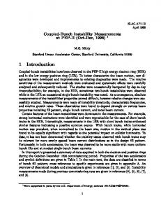
You will notice that there are two possible instances of Maxima called XMaxima and wxMaxima. While both allow the user access to the Maxima commands, the difference is in the graphic user interface (GUI) used to communicate with Maxima. XMaxima An example of the XMaxima interface is shown in Figure 1.1. The top of the GUI is the input window for Maxima commands. The lower part is a display of a Maxima Primer document providing the user with some information about getting started with Maxima. In between the top and lower part of the display you will find buttons labeled File, Back, 1-1

© Gilberto E. Urroz, 2008

Forward, Edit, Options, and Url: The last button refers to the file specification shown in the field immediately to its right. In this case, the file specification reads: file:/C:/PROGRA~/MAXIMA~1.0/share/maxima/514~1.0/xmaxima/INTRO~1.HTM The full reference to this file should be: file:/C:/Program Files/Maxima-5.14.0/share/maxima/5.14.0/xmaxima/intro.html The XMaxima GUI abbreviates some of the sub-folders in the first file specification producing the reference shown above, which could be a bit confusing. The full file specification shows the location of the file being shown in the bottom window of the XMaxima GUI. This html file is located in the Maxima installation as indicated above.

Figure 1.1. XMaxima starting GUI

1-2


The Back and Forward buttons allow the user to move about the document, while the other buttons provide the following menu items:

Using the Maxima Primer Scroll down the Maxima Primer document to learn about the use of Maxima. One of the first applications is presented in the following paragraph (lifted from the document):

Double-click on the integrate command shown in the Maxima Primer to see Maxima in action in the XMaxima window. The top window will now show the following operation:

Notice that there are two input locations labeled (%i1), or input 1, and (%i2), or input 2. Input 1 (%i1) is missing any input. This is so, because by double-clicking the integrate line 1-3


in the Maxima Primer, we activated the input without copying it to the top window. The result, however, is available in the top window as output 1 (%o1). Also, notice that XMaxima presents the result of the integral as closely as possible as a two-dimensional mathematical expression, i.e., 2 x - 1 atan(-------) log(x - x + 1) sqrt(3) log(x + 1) - --------------- + ------------- + ---------6 sqrt(3) 3 2

(%o1)

as opposite to a one-dimensional mathematical entry, i.e., -log(x^2-x+1)/6+ atan((2*x-1)/sqrt(3))/sqrt(3) + log(x+1)/3.

The full mathematical operation calculated in this example can be, on paper, written as

dx

∫ 1x 3 =−

2

ln  x −x1  6

tan−1





2∗x −1 3 log  x1 .  3 3

The user is invited to continue reading the Maxima Primer document and double-click on the different examples listed to learn the basic operation of Maxima. Following those exercises, one may notice, for example, that in the XMaxima interface, the mathematical constant π (the ratio of the length of a circumference to its diameter) is referred to as %pi. Also, infinity (∞) is referred to as inf. The Maxima Primer examples include also plots that are produced in their own separate graphics window, e.g., the commands ● ●

plot2d(sin(x),[x,0,2*%pi]) plot3d(x^2-y^2,[x,-2,2],[y,-2,2],[grid,12,12])

produce, respectively, the two-dimensional and a three-dimensional graphs shown below.

1-4


Click-off the graphical windows before continuing with the other commands in the Maxima Primer. wxMaxima wxMaxima uses an interface as shown in Figure 1.2, below.

Figure 1.2. The wxMaxima GUI. This interface is more sophisticated than that of XMaxima for the following reasons: ● ● ● ● ● ● ●

wxMaxima produces true two-dimensional mathematical output wxMaxima provides most Maxima commands in menus (e.g., Equations, Algebra, etc.) Some commands can be activated by using the buttons shown at the bottom of the interface, e.g., Simplify, Factor, etc. wxMaxima provides dialogues to enter parameters of selected commands. wxMaxima maintains a command line history buffer where previously used commands can be accessed, repeated, or edited. wxMaxima allows mixing text with mathematical expressions to produce printable documents. The current version of wxMaxima supports simple animations (to see the current version use the menu item Help > About). 1-5


A web page for wxMaxima is available here: http://wxmaxima.sourceforge.net/wiki/index.php/Main_Page For hints on the efficient use of wxMaxima visit: http://wxmaxima.sourceforge.net/wiki/index.php/Howto NOTE: Because of the additional features available in wxMaxima, we will use this GUI exclusively to present the examples contained in this and subsequent chapters. We will not be using XMaxima anymore in this or subsequent chapters. wxMaxima menus Take some time to explore the different menus in the wxMaxima GUI: ●

● ● ● ●

The File menu contains items typically found in windows-based applications such as Open, Read file, Save, Save As..., Export to HTML, Select File, Print, and Exit. Some items in the File menu, such as Load package, Batch file, and Monitor File, are proper of wxMaxima. The Edit menu contains typical commands such as Copy, Cut, and Paste, as well as others that are proper for wxMaxima. The Maxima menu contains items that allow the user to control the operation of Maxima. The Equations, Algebra, Calculus, Simplify, Plotting, and Numeric menus provide mathematical functions that are entered using dialogues. The Help menu contains several items of interest such as: ○ Maxima help: opens the Maxima Manual window with description and examples of Maxima commands. ○ Describe: produces a dialogue where the user can enter the name of a specific command. Try, for example, plot3d, and press OK. The dialogue will access the section of the Maxima Manual corresponding to the requested command. ○ Example: enters a series of examples of applications of the requested command into the wxMaxima interface. Try, for example, integrate, and press OK. ○ Apropos: use this dialogue to enter a keyword to search for a command that is similar to the keyword. For example, if you were seeking information on integration, you could enter the word integra, to get a listing of commands that may be related to integra. Then, you can use Describe or Example with one of the commands listed. ○ Show tip: shows tips on the use of Maxima. ○ Build info: provides information on the current version of Maxima. ○ Bug report: provides a web site where users can report errors in the operation of Maxima, or unexpected results of some operations. These “bugs” are reported to the programming team and solutions to them (if available) get incorporated in the new versions of the software. ○ About: provides the current version of wxMaxima. Notice that the versions of Maxima and vxMaxima are not necessarily the same. My installation, at the 1-6


moment of typing this book, showed Maxima version 5.14.0 and wxMaxima version 0.7.4. Remember that Maxima is the computer program that performs the mathematical calculations, while wxMaxima is the graphics user interface (GUI). wxMaxima tool bar The wxMaxima GUI provides a tool bar with the following buttons:

(1) Open session (2) Save session (3) Print document (4) Configure wxMaxima (5) Copy selection (6) Delete selection (7) Insert text (8) Insert input group (9) Interrupt current computation (10) Show Maxima help (same as menu item Help > Maxima help) Using the INPUT line The INPUT line in the wxMaxima interface can be used for a variety of purposes such as: ● ● ● ● ● ●

To To To To To To

perform a calculation, e.g., sqrt(1+3.5^2)/sin(%pi/6); define one or more variables, e.g., a:2; b:2; define a function, e.g., f(x):=sqrt(1+x^2); evaluate a function, e.g., f(2/3); produce a plot, e.g., plot2d(f(x),[x,-2,2]); enter other type of operations, e.g., a derivative: diff(t^2*sin(t), t);

Here are some observations from the examples shown above: ● ● ●

To enter the value of a variable use a colon (:) To define a function use a colon followed by the equal sign (:=) Maxima expressions end with a semi-colon. If you forget to enter the semi-colon in the INPUT line, wxMaxima will enter it for you.

This is additional information useful when entering expressions: ●

Variable or function names must start with a letter, and may include letters, numbers, and undersign, e.g., vx:2; x2:3; y_2:5; Initial_Velocity:-2.5;

1-7


●

The following are reserved words in Maxima and cannot be used as variable names: integrate in for else unless step

next at and do product

from limit elseif or while

diff sum then if thru

Some pre-defined functions: Some of the common pre-defined functions in Maxima include: sqrt tan csc atan acsc sinh asinh floor float

square root sin sine tangent cot cotangent cosecant asin inverse sine inverse tangent acot inverse cotangent inverse cosecant exp exponential hyperbolic sine cosh hyperbolic cosine hyperbolic asin acosh hyperbolic acos integer below ceiling integer above conver to floating point

cos cosine sec secant acos inverse cosine asec inverse secant log natural logarithm tanh hyperbolic tangent atanh hyperbolic atan fix integer part abs absolute value

Maxima does not have a logarithm-base-10 function. Instead, use:

log 10  x =

log  x  log 10

Here are some examples you can try: sin(2.5*%e);float(sin(2.5*%e)); floor(%pi);ceiling(%pi); log(5);float(log(5)); k:float(log(3)/log(10)); float(10^k);abs(-2);fix(3.3);fix(-3.2);

Notice that Maxima will tend to give symbolic results (i.e., results including fractions, square roots, unevaluated trigonometric, exponential, or logarithmic functions) rather than floating-point (or numerical) results. Use function float, as in the examples above, to get floating-point solutions. Automatic parentheses. Whenever you enter an opening parenthesis in the INPUT line, a closing parenthesis is added automatically. If you are not used to this feature, you may end up entering more closing parentheses than needed. This situation will result in an error that is easy to spot.

1-8


The percentage (%) operator.The percentage (%) symbol represents the most recent result. Try these examples: exp(-2.5)*sin(3*%pi/11);float(%);exp(-3);float(%);log(5);float(%);

To access the second-to-last commans use %2, the third-to-last, use %3, and so on. Mathematical constants. Some of the common mathematical constants available in Maxima are: %e %i inf minf infinite % phi % pi %gamma false, true

base of the common logarithms (=exp(1)) imaginary unit (=sqrt(-1)) real positive infinity real negative infinity complex infinity the golden ratio (φ) ratio of length of circumference to its diameter (π) Euler's constant (γ) boolean values (or logical values)

Here are some examples to try (in some examples we use function is to check whether comparisons of numbers are true or false): float(%phi);float(%pi);float(%e);%gamma; is(3>2);is(3 Save As ... and give a name to the file into which you will save your session. The following dialog form was used in a Windows Vista environment to save the current session.

The file storing the session will be located in the folder ../Documents/MAXIMA/, and will be named myFirstMaximaSession.wxm.

1-24


Reloading your session Restart Maxima (Edit > Restart Maxima) and use the menu item File > Open to browse your computer file system. For example, in a Windows Vista environment, I located the file I want to load in the following dialog form:

In this case, Maxima opens the file and executes every command, stopping at input (%i15) where it asks again about the value of coefficient w in variable myODE1. Repeating the response nonzero allows Maxima to continue evaluating the file to recover the entire session saved. Printing your session To produce a hard-copy of your session use the menu item File > Print. Loading a session without executing it An alternative way to load a saved session is by using the menu item File > Read File. Using this option will list all the commands in the session without executing it. The commands will be available in the command history, and could be reactivated by using the up- and down-arrow keys, and pressing [ENTER] when the proper command is in the INPUT line. Interrupting a calculation If, for some reason, wxMaxima seems to be hung up in a calculation, you can interrupt the processing by using the menu item Maxima > Interrupt, or type Cntl-G. Alternatively, use the interrupt button in the menu bar:

1-25


Ending your session To end your session use the menu item File > Exit, or click the [x] in the upper right corner of the wxMaxima window. This action produces the dialog form shown below.

Select [OK] if you don't want to save your current session. Otherwise, press [Cancel], save your session as indicated above, and exit wxMaxima once more. Formatting your session This section includes some examples of the use of text for commenting your session, as well as inserting sections and titles in your session. Inserting text (comments) in wxMaxima To enter text in wxMaxima use the menu item Edit > Insert > Text. The characters /* will be shown above the next input reference. Type one or more lines of text at the current cursor location. This line (or lines) of text can be used to comment your session. An example is shown next:

Text lines contained in saved session files get loaded with the rest of the commands when using File > Open or File > Read file. Inserting a title or a section in wxMaxima To insert a title use the menu item Edit > Insert > Title. This operation is similar to inserting text, except that the text is provided in a larger font. To insert a section use the menu item Edit > Insert > Section. This operation is also similar to inserting text, except that the text is provided in a larger font and with an underline. The following example shows a title and a section insertion in a wxMaxima session.

1-26


Inserting input The menu item Edit > Insert > Input produces a prompt input as illustrated in the following example:

If you enter a new command in the INPUT line, then the statement in front of the input prompt remains unevaluated. However, if you click on the input prompt statement, thus selecting it, and do a right-click, you can evaluate the command by selecting the option Re-evaluate input. In this case, the input gets evaluated as follows:

Clearing the screen The option Edit > Clear screen clears the current wxMaxima screen, showing at the top of the screen the current input reference, e.g.,

1-27


Additional session management in wxMaxima In this session we explore some of the menu items under the Maxima menu, namely: ● ● ● ● ● ● ●

Clear memory: clears all variables user-defined functions - equivalent to kill(all); Add to path: allows user to select folders to add to the search path for Maxima Show functions: lists all user-defined functions in the current session (functions;) Show definition: provides a dialogue form to request function definitions in session Show variables: lists all variables active in the current session (values;) Delete function: delete selected user-defined function or functions Delete variable: delete selected variables

The following example shows the definition of variables and functions and the listing of their names:

The option Show definition is used next to find the definition of function f2:

The result is shown below:

1-28


The option Delete functions produce the dialogue:

To delete functions f1 and f2 we enter those names in the dialogue. The result is shown below:

The option Delete variables produces the following dialogue:

To delete functions x1 and x2 we enter those names in the dialogue. The result is shown below:

An alternative way to delete user-defined functions or variables is to use function kill. This function basically clears any value or definition associated with a variable or function name. For example, to clear the contents of variable y1, use:

Check that the value of y1 is cleared:

1-29


Creating a batch file In an earlier exercise we saved a file called myFirstMaximaSession.wxm. In this section we will show you how to create a Maxima batch file out of your saved session. In order to create a batch file we need to edit the session file using a text editor. In this example I will use the Notepad++ text editor to open the session file. Notepad++ is available at http://notepad-plus.sourceforge.net/uk/site.htm .

When opened with Notepad ++, the file myFirstMaximaSession.wxm looks as follows:

Notice that you are warned in the very first line of the file to not edit the file by hand. This is for the wmx file. If you change anything in the file it may not be readable by wxMaxima again. The way to proceed is to save the file as a batch file, with the .mac suffix. Save it, for example, as myFirstMaximaBatchFile.mac, and edit it to look as shown below. This is the batch file that includes a number of comment lines (text between /* and */), and Maxima commands.

1-30


To load a batch file use the menu item File > Batch file, and select the proper file to load. The result of the batch file operation will be shown in your wxMaxima window. Notice, however, that the comment lines are not shown in the wxMaxima window. If you want to show explanatory text from your batch file, you may want to replace the comments by a string, making sure that the string ends in a dollar sign ($) rather than in a semi-colon (;).

1-31


With theses changes, the output in the wxMaxima is now well documented, although the comment strings are now part of the input (with no output), rather than inserted text. Part of the output from the batch file is shown below:

A batch file can also be created from scratch. Simply type the Maxima commands in a text file and save it with the suffix .mac. Here is an example of a batch file created from scratch:

1-32


Important basic functions This section addresses a few basic functions and operators of general application in mathematical functions and that were not addressed in any of the previous sections. Evaluation or not evaluation of an operation In many of the examples presented above related to differential equations we use an apostrophe (') in front of the derivative operator, diff, in order to avoid its evaluation. To illustrate the difference between the entry 'diff and diff, see the following example:

In the first expression, using 'diff(x,t,2) produces as output the derivative thus indicated. However, in the second expression, Maxima evaluates the required derivatives. Since function x(t) has not been defined, the derivatives in the second expression evaluate to zero, and the result is x = e-t. The following example shows an non-evaluated integral:

An example of a summation is shown next:

Applications of ev Function ev evaluates an expression in a given environment determined by a number of arguments. For complete information on function ev, use the menu item Help > Describe, and enter the name ev in the dialogue form. In this document we will present only some specific examples of the use of function ev. 1-33


●

Substituting constants in an equation before solving it:

●

Force floating-point evaluation of rational numbers:

●

Force derivative calculation after result has been suppressed:

●

Derivative and integral calculations can be forced with the option nouns:

These examples illustrates how to list an expression and their evaluation in the same line. It also introduces the idea of nouns in Maxima evaluation.

1-34


Nouns and verbs To understand the use of the argument nouns in the examples above, please open the Maxima Manual, available through the menu item Help > Maxima help, and find section 6.3 Nouns and verbs in the Contents tab, as shown in the figure below.

Read this section in the Manual to understand the idea of verbs and nouns, as well how to convert form one to the other.

Online help In an earlier section we presented the different options available in the Help menu. A quick way to obtain help is by using the ?? operator. For example, if you are interested in finding information about the function eval, use:

Maxima reply by listing a number of entries that include the particle eval, and requesting additional input from the user. At this point, the user can enter a particular number referring to the 7 options listed, or enter the particles all or none. Enter none to stop the online help process.

1-35


The following is another example related to the function integrate.

1-36


Real numbers, functions, and units in Maxima In this Chapter we introduce calculations with real and complex numbers using Maxima. We also introduce the use of functions, conditional statements, and logical particles. This chapter also includes examples of calculations using units of measurements. Symbolic and floating-point results with real numbers In this section we present simple calculations with real numbers and introduce conversion from symbolic to floating-point results. Symbolic results represent the results that one would obtain by working by hand, and producing simplification of operations with numbers. By default, Maxima produces symbolic results when operating with real (and complex) numbers. To produce floating-point values it is necessary to use function float as illustrated in the examples shown below. Notice that the first example shows a simple fraction of integer numbers, while the second example shows a square root calculation.

Fractions involving floating-point numbers produce floating-point results, e.g.,

Changing the default format Use the menu item Numeric > Toggle numeric output to change the default format of calculations with real numbers. For example, activating this item once, changes the default output format to floating point as illustrated below.

2-1

© Gilberto E. Urroz, 2008N

A second application of the menu item Numeric > Toggle numeric output will return the default output format to symbolic:

In this specific example the output %e-2 is the symbolic representation of the number e-2, while 0.1353... is the corresponding floating-point result. Other format changes The Numeric menu includes also the menu items Numeric > To float and Numeric > To bigfloat that can be used to convert a symbolic result into either a simple floating-point format, or to a double-precision floating-point format (referred to as bigfloat in Maxima). These two menu items are equivalent to the functions float and bfloat, respectively. When applying any of these two menu items, the result refers to the last result available (i.e., to %). The following two examples show the application of To float and To bigfloat to the number e-2.

Notice that the last result is in power-of-ten format with b indicating the power of ten. While the output shown uses the default number of digits (16), the value is stored in a double-precision location. Power-of-ten format To enter power-of-ten floating-point values use e to indicate the power of ten, some examples are shown below:

2-2


If entering a power-of-ten floating-point number using b instead of e, the number will be stored as a bigfloat number. Some examples are shown below:

Combining float and bigfloat numbers results in a bigfloat number, e.g.,

Setting floating-point precision By default, Maxima shows 16 digits in a floating-point number. Using the menu item Numeric > Set Precision ... produces a dialog form where you can enter the precision (number of digits) to show in your floating-point results, e.g.,

A simpler way to change the precision is to redefine parameter fpprec. In the following examples we change fpprec to values of 16, 32, 64, and 128, and then display the value of p %pi) using function bfloat:

2-3


Calculations with real numbers In this sections we present calculations with real numbers involving not only simple arithmetic operations (+, -, *, /, ^), but also square roots (sqrt), other roots, absolute values (abs), trigonometric functions and their inverses (sin, cos, asin, acos, etc.), hyperbolic functions and their inverses (sinh, cosh, asinh, acosh, etc.), exponential (exp), natural logarithms (log – note: not ln), ceiling, floor, fix, and float. By default symbolic results will be provided. Use function float to obtain floating-point results. Please notice that the arguments of trigonometric functions are in radians, the natural angular unit. To convert from degrees to radians use the factor %pi/180. Try some of the following examples (see the results in your own Maxima installation): 2+(1/(2+1/(2+1/2))); 4./3.+3./4.+1./6.; sqrt(1+(3/2)^3); abs(-2.5+1/2.5); sin(%pi/3+cos(%pi/3)); sqrt(exp(-2)+log(abs(-2+1/2))); ceiling(3.25); floor(3.25); fix(3.25); 3.25-fix(3.25); sinh(2.5);

Evaluation of formulas Evaluation of formulas is a common application of real number calculations. I suggest using a three-step approach: 1. Enter formula (remember to use : instead of =) 2. Enter list of values known, separated by $ to avoid taking space in the window 3. Use the command history to repeat the formula expression, which is now evaluated If need be, use float(%) to obtain a floating-point value. Some examples are shown below. Example 2.1:

2-4


Example 2.2:

Note: in this last example, kill(all) was used to clear all existing values. Also, the intermediate equation A2:float(%pi*D2^2/4) is calculated before calculating the value of Q. Defining functions To define a function write the function name and arguments, e.g., f(x), g(y), h(x,y), followed by := and by the function definition. Evaluation of the functions is performed by replacing the unknowns with variable names or numerical values.

Defining a function as a sequence of expressions Suppose that you want to define a function given by the following expression: f  x =

2 x 33x 3 2   x 3x  2 2 x 4 x 4

2-5


Notice that the definition of the function includes a couple of groupings of expressions, namely, (x2+4) and (x3+3x), that appear twice in the expression for f(x). It could be possible to calculate the function in three steps, namely, ● ● ●

a = x2+4 b = x3+3x 2 b f  x =  b 2 a a

In Maxima, we can define a function such as this by using a sequence of expressions separated by commas. For example,

Check the full expression of the function by using, for example, f(t):

Evaluation of the function is straightforward as illustrated in the following examples:

Using function ratsimp - Function ratsimp (rational simplification) can be used to simplify rational expressions such as fractions, polynomials, etc. This function will be presented in a later chapter in reference to simplification of algebraic expressions. It is introduced here to show an alternative way to define the function presented above:

2-6


The function definition is now:

In this case, evaluation of the function with algebraic arguments will produce a fully expanded expression, e.g.,

Defining functions with a block statement Functions that require more than one statements to be defined can use the block statement. The block statement is used if a return statement is to be included. The general form of a block-statement function is as follows: block([], )

To illustrate the use of the block statement in defining a function, consider the function:

{

x1,if 0≤x2 f  x =  x12 , if 2≤ x4 0, elsewhere

}

.

Using the Multiline Input - To enter the command defining the function we will use the Multiline Input window, available by clicking the multiline icon available at the end of the INPUT line in the wxMaxima window . Clicking this icon produces the following window, in which we enter the definition of function f(x) using an if-then command, and an if-then-else command as shown:

2-7


Using vectors - To illustrate the operation of the function we will generate a vector of data by evaluating the function at points x = -2, 0, 1, 2, 3, 4, and 5, i.e.,

The if-then and if-then-else constructs – In the definition of function f(x) shown above, we used both an if-then and an if-then-else constructs. The if-then construct has the general form: if then The result from this construct is to perform the if the is true, or do nothing otherwise. On the other hand, the if-then-else construct has the general form: if then else The result from this construct is to perform if the is true, or perform if the condition is false. Conditional statements – Conditional statements are statements that result in a true or false outcome. Numerical comparisons are common forms of conditional statements. In the definition of function f(x) used conditional statements such as: 2Complex simplification sub-menu. Convert to rectform This menu item converts a complex expression into its rectangular form. This command can be used to show the results of complex number operations, as illustrated in these examples. First we define two complex numbers z1 and z2 and attempt an addition:

Using the Convert to rectform (rectform) command we get:

The following examples show the command rectform applied to subtraction, multiplication, division, and powers of complex numbers:

3-16


Using actual numbers:

Convert to polarform This menu item converts a complex expression into its rectangular form. This command can be used to show the results of complex number operations, as illustrated in these examples. First we define two complex numbers z1 and z2 as follows:

In this case we use sub-indices to define the variables theta[1] and theta[2]. The sum of the two complex numbers is a long expression in its polar form:

3-17


Multiplications, divisions, and powers will show more manageable expressions, although the user needs to reply to additional requests for information from Maxima:

The following examples use actual numbers:

3-18


Get real part This menu item extracts the real part of a complex variable or expression:

Get imaginary part This menu item extracts the imaginary part of a complex variable or expression

Demoivre The simplest application of this menu item (demoivre) is to implement De Moivre's formula, e i =cos i sin , i.e.,

Other examples are shown below:

3-19


Exponentialize This menu item is the inverse of the Demoivre menu item, producing the exponential form of complex expressions involving trigonometric and hyperbolic functions, e.g.,

These two expressions, for example, show the definitions of the functions sin(z) and cosh(z) in term of the real and imaginary parts, x and y. More functions for complex numbers Maxima includes the following functions for manipulation of complex variables or expressions: ● ● ● ●

cabs carg conjugate residue

-

complex absolute value (modulus) complex argument complex conjugate residue in complex plane

While the modulus (cabs) and argument (carg) have been defined before, in this section we include definitions related to the functions conjugate and residue shown above. The complex conjugate of the complex number z = x + iy = reiθ is the reflection of z about the x-axis, i.e., z = x – iy = reiθ. The product of a complex numbers and its conjugate is the square of its modulus: z ⋅z = x2 + y2 = |z|2 = r2.

3-20


The following examples cover applications of the functions cabs, carg, and conjugate for complex expressions:

A Laurent series expansion for a complex expression requires a point of expansion z0. The Laurent series resembles a Taylor series expansion but it includes both positive and negative powers. The residue of a complex expression is the coefficient of the power (-1) term in the expansion of the expression in a Laurent series. For additional information on Laurent series check out the following online links:

● ●

Wikipedia link: Wolfram Mathworld link:

http://en.wikipedia.org/wiki/Laurent_series http://mathworld.wolfram.com/LaurentSeries.html

Function residue requires the complex expression being expanded, the complex variable, and the point of expansion, and returns the residue in the complex plane for the expression. Examples:

3-21


Substitution and other menu items for expression manipulation The last set of functions in the Simplify menu include the following items:

Substitute... This menu item activates a dialogue form that allows the substitution of a variable into an expression. For example, the following two examples show the dialogue form and the resulting entry into the wxMaxima window:

Checking the [ ] Rational box in the the dialogue form implements function ratsubst (rational substitution) rather than subst alone. The difference, in this example, is that a rational simplification is applied to the resulting expression. Here is another example:

3-22


An alternative way to use function subst is to create a list of substitutions using equal signs, as illustrated in these examples:

Evaluate noun forms Noun forms, as opposite to verb forms, are executable expressions in Maxima that remain unevaluated. The item menu Evaluate noun forms allows the evaluation of those unevaluated expressions. To produce an unevaluated expression typically you precede it with an apostrophe. Some examples of unevaluated expressions, and their result after the Evaluate noun forms menu item is activated, are shown below:

Toggle algebraic flag The Maxima Manual (select it using Help > Maxima help) has a simple entry for the algebraic flag. The Manual indicates that the default value of the algebraic flag is false, and that it must be set to true (using, algebraic : true) “in order for the simplification of algebraic integers to take effect.” By using this menu item you can toggle the algebraic flag between true and false. To find out about the current setting use (default set):

3-23


Add algebraic equality... This menu item activates the tellrat function to produce algebraic equality between expressions. Refer to the Maxima Manual for the operation of this function. Activate the Maxima Manual using Help > Maxima help, click on the Index tab, and type tellrat:

Modulus computation... The menu item Modulus computation... allows the user to set the modulus for modular arithmetic calculations. The default value is false. The user can set the modulus value to an integer value, say, 2, 3, etc. Typically the modulus is a positive prime number. The following references address the issue of modulus arithmetic:

● ●

Wikipedia link: http://en.wikipedia.org/wiki/Modular_arithmetic Wolfram Mathworld link: http://mathworld.wolfram.com/ModularArithmetic.html

Some examples of modular arithmetic calculations are shown below. First, examples with modulus = 3:

3-24


The second set of examples correspond to modulus = 5:

Simple operations with polynomials In this section we provide examples of functions that apply to polynomials. coeff The coeff function, coeff(p,x,n), is used to extract the coefficient of the variable x of order n in the polynomial p:

divide (also Calculus > Divide polynomials...) The divide function, divide(p,q), produces the quotient and residual of the polynomial division p/q:

3-25


quotient, and remainder The quotient and remainder functions, quotient(p,q) and remainder(p,q), produce, respectively, the quotient and residual of the polynomial division p/q:

ratdiff The ratdiff (rational differentiation) function, ratdiff(p,x), produces the derivative of a rational function p with respect to variable x:

allroots (Equations > Roots of polynomial) The allroots function, allroots(p) or allroots(p,x), calculates all the roots x of a polynomial p:

realroots (Equations > Roots of polynomial (real)) The allroots function, realroots(p) or realroots(p,x), calculates the real roots x of a polynomial p:

3-26


gcd (Calculus > Greatest common divisor... ) The gcd function calculates the greatest common divisor for two or more polynomials, e.g.,

Let's add one more polynomial to the gcd function:

Function gcd can also be applied to integers:

horner Function horner produces the expression corresponding to the Horner's rule for evaluating polynomials. The following example shows the Horner's rule for a list of two polynomials:

lcm (Calculus > Least common multiple ...) The lcm function calculates the least common multiple for two polynomials, or integers. This function belongs to the functs package, which must be loaded before applying the function. Function lcm can be invoked from the Calculus menu, however, before using this menu item it is necessary to load the functs package. Thus, the first command to enter is: 3-27


The following example shows function lcm applied to pairs of numbers:

Next, we apply function lcm to a pair of polynomials:

NOTE 1: Function lcm belongs to package functs which contains a number of other useful functions that apply to polynomials and numbers. The contents of package functs are presented in a section at the end of this Chapter. NOTE 2: For additional information on polynomials activate the Maxima Manual (Help > Maxima help) and find the Polynomial chapter in the Contents tab.

3-28


Simple operations with fractions In this section we provide examples of functions that apply to fractions. combine The combine function can be used to collect fractions with the same denominator:

partfrac (Calculus > Partial fractions...) The partfrac function decomposes a single fraction into its partial fractions:

cfdisrep (Calculus > Continued fraction) The cfdisrep function is used to produce a continued fraction given the coefficients of those fractions as illustrated in this example:

3-29


Functions in the functs package This section presents examples of functions in the functs package. The descriptions of the functions was taken from the Maxima online help facility for functs, i.e.,

Interestingly enough, function lcm, which was presented in an earlier section, is not included in the help entries for functs. rempart (expr, n) Removes part n from the expression expr. If n is a list of the form [l,m] then parts l through m are removed.

wronskian ([f1, ..., fn], x) Returns the Wronskian matrix of the functions f1, ..., fn in the variable x. f1, ..., fn may be the names of user-defined functions, or expressions in the variable x.

3-30


tracematrix(M) Returns the trace (sum of the diagonal elements) of matrix M.

rational(z) Multiplies numerator and denominator of z by the complex conjugate of denominator, thus rationalizing the denominator.

A similar result is obtained by using function rectform:

gcdivide(p,q) When takegcd is true, gcdivide divides the polynomials p and q by their greatest common divisor and returns the ratio of the results.

3-31


When takegcd is false, gcdivide returns p/q.

arithmetic (a,d,n) Returns the n-th term of the arithmetic series a, a+d, a+2d, ..., a+(n-1)d.

geometric (a,r,n) Returns the n-th term of the geometric series a, ar, ar2, ..., arn-1.

harmonic (a,b,c,n) Returns the n-th term of the harmonic series a/b, a/(b+c), a/(b+2c), ..., a/(b+(n-1)c).

arithsum (a,d,n) Returns the sum of the arithmetic series from 1 to n.

geosum (a,r,n) Returns the sum of the geometric series from 1 to n. If n is infinity (inf) then a sum is finite only if the absolute value of r is less than 1.

gaussprob (x) Returns the Gaussian probability function `%e^(-x^2/2)/sqrt(2*%pi)', i.e., the standard normal probability density function (pdf). 3-32


Here is a list of ordinates of the standard normal pdf:

Here is a list of probabilities of the intervals -1 < x < 1, -2 < x < 2, and -3 < x < 3, respectively,

Notice that integrals of the gaussprob(x) function are given in terms of the error function (erf). To find out about the error function check the Maxima online help:

Finally, a plot of the standard normal pdf is shown below: 3-33


gd (x) Returns the Gudermannian function `2 * atan(%e^x - %pi/2)'.

agd (x) Returns the inverse Gudermannian function `log (tan (%pi/4 +

x/2)))'.

vers (x) Returns the versed sine `1 - cos (x)'.

3-34


covers (x) Returns the coversed sine `1 - sin (x)'.

exsec (x) Returns the exsecant `sec (x) - 1'.

hav (x) Returns the haversine `(1 - cos(x))/2'.

3-35


Basic plotting commands in Maxima In this Chapter we present examples of plotting commands in Maxima useful for the creation of two-dimensional and threedimensional graphics. The plot2d command The plot2d command, in its simplest form, requires as input an expression or function name, and a range of values of the independent variable. Consider the following example typed in a wxMaxima window:

By default, this command produces a plot in a gnuplot window, as shown below for a Windows Vista environment:

In a Linux environment, specifically a Fedora 7 Linux environment, the following Gnuplot window would be produced:

4-1


In the wxMaxima window a plot can be produced inline by using the command wxplot2d, e.g.,

NOTE: It will be more accurate to say that to produce an inline two-dimensional plot you need to use the wx “wrapper” with the plot2d command, rather than referring to a wxplot2d command. Specifying the vertical range Besides specifying the abscissa or horizontal range (i.e., the x range), the plot2d command allows the user to specify the ordinate or vertical range (i.e., the y range). Consider the following two examples:

In the first case no vertical range is specified, thus, Maxima will tend to include the default vertical range [0,10]. In the second case, the vertical range [y,0,5] is specified, thus reducing the vertical range to half of that in the first case.

4-2


The following example illustrates the case of the function sec(x) which takes positive and negative infinite values at certain points. Without specifying the vertical scale the graph does not show much detail of the curve, i.e.,

The function diverges at values of -p/2 and p/2 as indicated by the vertical lines. The default vertical range extends from -250,000 to 50,000, a very large range indeed. Specifying a smaller vertical range,say -20 < y < 20, allows the user to see the details of the curve behavior:

4-3


Plotting more than one curve Specifying a list of functions or expressions allows the plotting of more than one curve through the use of plot2d (or wxplot2d), e.g.,

Specifying legends for multiple curves In the example above, the plot shows the function expressions as the legends for the two curves. The user may specify the legends to be included by using the legend option as illustrated in the following example:

4-4


Specifying labels for the plot The following example illustrates the use of the options xlabel and ylabel to specify plot labels:

The following example illustrates the specification of vertical scale, legends, and labels:

4-5


Plotting discrete data The examples shown above, where the curves plotted are based on expressions or functions, produce, by default, smooth, continuous lines. If the data to be plotted consists of discrete data points, say,

one can use the discrete option, altogether with the list of data points x and y, to produce a plot, e.g.,

Style: points - The resulting plot shows a series of segments joining the individual points corresponding to the data in lists x and y. The continuous line is the default plot style. In order to produce discrete points use the option [ style, [points] ], e.g.,

4-6


The points option for style can have one, two, or three additional options of the form: [points,radius,color,object]. The first option, radius, represents the radius of the points to be plotted. The larger the value of this first parameter the larger the individual point symbols. The second option, color, represents the color of the points with default values: 1-blue

2-red

3-magenta

4-orange

5-brown

6-lime

7-aqua

The sequence of colors repeat after the number 7, i.e., 8 will be blue, 9 red, etc. The last option, object, in the points specification represents the type of symbol, or object, that will be plotted, according to the following codes: 1: filled circles 4: times sign (x) 7: open squares 10:filled inverted triangles 13: open lozenges.

2: open circles 5: asterisk (*) 8: filled triangles 11: open inverted triangles

3: plus signs (+) 6: filled squares 9: open triangles 12: filled lozenges

The following figure illustrates three different point sizes (1, 10, 3) and two different colors (2 – red, 7-acqua):

4-7


The following examples show different combinations of the three options for points:

Style: lines – As with the case of points, the style option lines can alter the appearance of continuous lines by using the form [lines,[thickness,color]]. The option thickness operates similar to radius for points, while the option color is the same as in points. Some examples are shown below:

4-8


The lines option can be used with plots of functions or expressions, e.g.,

Styles: linespoints – This style combines lines with points and can use up to four options: [linespoints,[line thickness, point radius, color, object]]. Both lines and points will have the same color. Some examples are shown below:

Style: dots – This option shows discrete points a individual dots. These dots are a singlepixel size, therefore, they're hard to see in the plot, e.g.,

4-9


Plotting multiple types of data The following examples illustrate the plotting of different types of data. We start by showing a plot of a continuous function together with discrete data. The first case shown illustrates the use of two different styles, one for the continuous line, and one for the discrete data points. The second case illustrated shows the use of two different styles, plus a legend specification.

The next example shows how the same set of discrete data can be plotted simultaneously as a line and points. This is similar to the plot of the single discrete data set with the single style linespoints, except that the latter forces both lines and points to be the same color.

4-10


Plotting parametric plots Function plot2d can be used to plot parametric plots as illustrated in the following example:

Notice that the specification of a parametric plot requires the word parametric, and the expressions for the x and y components for the curve. The range of the independent variable is also required. Notice that, by default, the parametric plot used only 10 points to draw the curve. This situation can be improved using the plot option nticks. By making nticks to be 200 a smooth curve is produced for the parametric equations x = sin(t), y =cos(t)/2. The next example shows a parametric curve and a discrete data set plotted in the same set of axes, including different styles and a legend option.

4-11


The next example shows a plot combining a function plot, a parametric plot, and a discrete data set:

The next example is the same as above, in terms of the plots, but including labels for the axes:

4-12


Logarithmic scales Adding the option [logx,true] will force the x axis scale to be logarithmic, whereas the option [logy,true] will force the y axis scale to be logarithmic. Some examples are shown below. First, an example of a semi-logarithmic plot with the x scale being logarithmic. Notice that the option [logx,true] automatically produces the label log(x) in the x axis.

The following example illustrates the use of the [logy,true] option to produce a semilogarithmic plot where the vertical scale is logarithmic:

4-13


A double-logarithmic, or log-log, plot is shown next:

The box option The box option is set to true by default. Changing it to false removes the frame from the plot, e.g.,

4-14


The plot_realpart option for complex numbers Using the option [plot_realpart,true] with the plot2d command allows plotting the real part of complex numbers. The result is equivalent to plotting realpart(x) where x may contain complex numbers. The default setting for plot_realpart is false, in which case, complex numbers are ignored in the plot. To illustrate the use of the plot_realpart option consider the following plots:

Gnuplot options As illustrated in the examples shown above, the output of function plot2d is a gnuplot window (or an inline gnuplot window if the wxMaxima wrapper is used, i.e., wxplot2d). In this section we present some plot options related the gnuplot window. Selecting the gnuplot terminal (gnuplot_term and gnuplot_out_file options) To change the gnuplot terminal use the option [gnuplot_term, terminal_type], where terminal_type can take the values:

●

default dumb ps

●

other

● ●

output is displayed in a gnuplot window or inline output is displayed in an old-fashioned dumb terminal generates a default PostScript file maxplot.ps, unless a filename is given using the option gnuplot_out_file png, jpeg, svg 4-15


The following examples illustrate the use of this option. First, we show the result of a ps option using the default PostScript file name:

I used Adobe Acrobat Distiller to convert this ps file into a pdf file, from which I extracted the following plot:

To produce a PostScript file with a specific name, one could use, for example:

An example of a dumb terminal output, including an output file, is shown below:

4-16


The following example shows a plot which is send to a jpeg file (myPlot1.jpg):

The resulting file can be opened with any graphics software (e.g., Paint in Windows Vista). The result was copied into this document as shown below:

The gnuplot_preamble option The gnuplot_preamble option is set to an empty string “” as default. The string can be replaced by a string containing a number of gnuplot commands to set up a number of plot format options. These options may include logarithmic scales, location of legend key, placing zero axes, and location of x and y ticks, as illustrated in the following examples. Zero axes – The first case presented shows the setting of zero axes in the plot ●

Default case:

●

Preamble set for zero axis in both x and y:

4-17


4-18


Location of legend key – Using the gnuplot_preamble option with value “set key bottom”, “set key left”, or “set key left bottom” allows changing the location of the legend key. The default location is the upper right corner. The following plots illustrate the four possible corner locations.

Other options for the location of the legend key are “set key center”, “set key top center”, “set key bottom center”, “set key left center”, and “set key right center”. Two of these cases are illustrated below.

4-19


Setting tics on axes – Use the options “set xtics( ...)” and “set ytics(...)” to set the tick marks in the x and y axes. The following example illustrates the use of this option. The figure to the left is the default setting for ticks, while the figure to the right shows userdefined settings for those ticks.

Controlling the wxplot2d inline size The size of an inline plot is controlled by the variable wxplot_size. By default, this value is the list [400,250], representing the horizontal and vertical sizes of the inline plot window in pixels. To change the size of the inline plot, therefore, redefine the variable wxplot_size accordingly. Try the following examples:

4-20


An example of a two-dimensional plot The specific energy in an open channel is defined as the energy per unit weight measured from the channel bottom. The equation that defines specific energy is:

where E = specific energy, V = flow velocity, g = acceleration of gravity, and y = flow depth. The flow velocity, in turn, is defined in terms of the unit discharge (or discharge per unit width), q, as V = q/y, and replaced into the energy equation as:

Next, we replace the values q = 10 ft2/s, and g = 32.2 ft/s2, and define a function E(y) using the right-hand side (rhs) of the equations EnerEqQ:

To see the expression for the function E(y) use:

The plot of this function is shown together with the line E = y.

4-21


Using lists for producing plots The graph of specific energy shown above is typically shown with the axes switched. One possible way to produce such a plot is to create a well-populated list of values of y and then generate the corresponding list of values of E(y). To create a systematic list of values we use function makelist. For example, for the function E(y) used above, we can generate lists of values of y (yList) and E (EList), as follows:

To produce the plot, we first change the inline plot size and then use the following plot2d command:

4-22


The plot3d command The plot3d command can be used to produce a surface plot of a function of the form z = f(x,y), e.g., produces the plot:

If you click on the gnuplot graph window and then hold the left-mouse button while moving the mouse it is possible to rotate the view of the three-dimensional plot, e.g.,

4-23


Using the openmath window An alternative display for plot3d (also available for plot2d) is the plot format openmath. The following example shows the use of openmath:

The resulting graph is shown in a Tk Schelter's 3d Plot Window as shown below:

The openmath window provides a number of buttons that allows the user to modify the plot format. The options for the Config button are shown in the figure to the right. The Zoom button prepares the plot to zoom in or out. The instructions for zooming are as follows: ● ●

Click to Zoom Shift+Click to Unzoom

The Save button allows the user to save the plot in a file (see next page). The Replot button replots the graph. The Rotate button prepares the plot for rotation using the mouse. The Azimut and Elevation angles will be shown. The Close button closes the figure. 4-24


Inline three-dimensional plot with wxplot3d Use function wxplot3d to produce an inline three-dimensional plot as illustrated in the figure below. The figure to the left uses the default inline window size of [400,250, while the figure to the right shows a larger inline window of size [400,400].

4-25


The grid option The grid option determines the number of points used in the x and y variables in the plot. The default value is [grid,30,30].

Removing the mesh To remove the mesh from the surface use the option [gnuplot_preamble, “unset surface”]. The following figure shows the default surface format to the left, and the surface without the mesh to the right.

Plotting a three-dimensional parametric curve To plot a parametric curve provide a list of three functions [x(t),y(t),z(t)], and two variable ranges, one being the parameter for the curve, in this case, [t, 0, 10], and the second one being a dummy variable, e.g., [s, 0,10]. Only the range [t,0,10] is used in the calculation of the curve, but plot3d will not work unless the ranges for two independent variables are given. 4-26


Plotting a parametric surface The approach followed to produce a parametric surface is the same as in a parametric curve, except that the functions provided are of the form [x(u,v), y(u,v), z(u,v)], with ranges for variables u and v. The following parametric surface is produced using the option [plot_format,openmath]:

Surface with projected contour plot Define a string variable: mypreamble : "unset surface; set contour; set cntrparam levels 20; unset key";

Then, use the [gnuplot_preamble,mypreamble] option.

4-27


Color map A color map, somewhat similar to a contour plot, can be generated by using the option [gnuplot_preamble, “set view map; unset surface”]. Increasing the grid size improves the smoothness of the color map.

Transformation from polar coordinates A parametric surface of the form [r,θ,rθ], with parameters [r,0,2] and [θ,0,π], is interpreted as a Cartesian (rectangular) surface, i.e., [x = r, y = θ, z = rθ], as in the figure to the left. If the intention is for the functions [r,θ,rθ] to represent the polar coordinates, i.e., [r = r, θ= θ, z = rθ], it is necessary to use the option: [transform_xy, make_transform([r,theta,z],r*cos(theta),r*sin(theta),z).

The result is shown in the figure to the right.

4-28


The function make_transform, used in the example above, can be used as the value for the option transform_xy for other type of transformations, e.g.,

The following figures demonstrate the plotting of a hemisphere using Cartesian coordinates and polar coordinates:

Contour plots Function contour_plot, with similar arguments as plot3d, produces contour plots of functions of the form f(x,y). The first example shown uses the default number of parameters: 4-29


The next two plots show the contourplots corresponding to 10 and 20 contour levels, as specified by the option [gnuplot_preamble, “set cntrparam levels 10”], etc.

4-30


The use of the grid option makes for smoother contours, e.g.,

4-31


Use of the Plot 2D... and Plot 3D... menu items/buttons The wxMaxima interface provides quick access to the Plot2D and Plot3D functions through the menu items Plotting > Plot 2D... and Plotting > Plot 3D... , respectively. Alternatively, one can use the Plot 2D ... and Plot 3D... buttons available in the interface:

The Plot 2D... form Activating the Plotting >Plot 2D... menu item produces the following dialogue form:

The different entry fields are interpreted as follows: ●

The Expression(s) field are used to enter an expression in terms of variable x, let's refer to it as f(x).

●

The suggested range for x is -5 Roots of polynomial) The function allroots is used to calculate all roots, both real and complex, in a polynomial equation. Some examples using function allroots are presented below. Example 5-9 – Repeating Examples 5.3 and 5.4 - To illustrate the use of function allroots we repeat the solutions to Examples 5.3 and 5.4 using such function:

5-11


realroots (Equations > Roots of polynomial (real)) Function realroots produces the real roots of a polynomial equation. Some examples of the use of realroots are presented below. Example 5-10 – Repeating Examples 5.3 and 5.4 - To illustrate the use of function realroots we repeat the solutions to Examples 5.3 and 5.4 using such function:

NOTE: Functions allroots and realroots require a specific polynomial to produce a solution. Thus, attempting a general solution (e.g., as in the quadratic equation in Example 5.1) will produce an error:

The following engineering examples refer to function allroots and realroots. Example 5-11 - Critical depth for a trapezoidal channel – The cross-section of a trapezoidal channel, as shown in the figure to the right, is characterized by its bottom width b, its depth of flow y, and its side slope z (i.e., zH:1V). You can show that the specific energy equation for this cross-sectional shape is calculated as:

The critical depth can be obtained by taking the derivative of the specific energy with respect to y, i.e.,

5-12


and, then, making dE/dy = 0:

An attempt to use function solve to solve this equation produces a re-arrangement of the previous result into a polynomial, although no solution is given:

Let's substitute the following parameters into the equation b = 5 ft, z = 1, Q = 200 ft3/s, g = 32.2 ft/s2:

Trying function solve after replacing the parameters still does not produce a solution:

Notice, however, that function solve recast the polynomial into one with all integer coefficients. Since the equation is indeed polynomial, we'll use function allroots to find the solution:

This attempt to solve the equation using function allroots still reports an error. The reason for the error is the fact that the content of variable SolC1 is a list (as indicated by the brackets [ ] enclosing the polynomial. Thus, to extract the actual polynomial it is necessary to use a subindex. Thus, try:

5-13


Alternatively, one can use realroots(SolC1[1]); to find only those real solutions, namely, y = 2.99 ft ≈ 3 ft, and y = -2.59... ft ≈ -2.6 ft. Only the first result, y = 3 ft, makes physical sense. Example 5-12 - Manning's equation for a trapezoidal channel – Consider an open channel of constant cross-section laid on a bed slope S0. The bed slope represents the drop in ft per ft of channel length. If uniform flow, or flow of constant depth, occurs in this channel, the mean flow velocity is calculated using the Manning's equation, EqMV:

This is an empirical equation developed by an Irish engineer by the name of Manning in the late 1800's. In spite of being totally empirical, it is the most popular equation to calculate uniform flow in open channels. It is widely used around the world, and is known in Europe as the Manning-Stickler equation. In the Manning's equation the parameter Cu is a constant that depends on the system of units used. If using units of the International System (S.I.), Cu = 1. If using units of the English System (E.S.), Cu = 1.486. The parameter n is known as the Manning's roughness coefficient and it depends on the type of lining for the channel (e.g., for concrete, n = 0.012). Finally, R is known as the hydraulic radius, and it's defined as the ratio of the cross-sectional area A to the wetted-perimeter P of the cross-section (i.e., the length of the cross-section perimeter 'wetted' by the water), thus, R = A/P. The Manning's equation can be combined with the continuity equation (conservation of mass) for a liquid (constant density), EqQ, where Q is the volumetric discharge through the cross-section:

When substituting the Manning's equation (EqMV) into the continuity equation (EqMQ) results in a Manning's equation based on the discharge, EqMQ:

Replacing the hydraulic radius, R, in terms of area A and perimeter P, EqMQ becomes:

5-14


For a trapezoidal channel, as shown in Example 5-11, the area and wetted perimeter are define below and replaced into equation EqMQ:

We will be solving this equation for the depth of uniform flow, referred to as the normal depth. We notice that the equation EqMQ has exponents 5/3 and 2/3 for the terms containing y. However, since the exponents are fractions with denominator 3, it is possible to convert the equation into a polynomial equation by first multiplying it out by the denominator of the right-hand side of EqMQ:

Then, we raise both sides of the equation to the third power:

Now all the terms involving y have integer powers (2 and 5) and could be expanded into a polynomial (although we don't actually expand the polynomial out in this solution)

Even without expanding the polynomial, we can use function allroots to get all 10 roots of the resulting polynomial (the order 10 comes from multiplying out the y5 term with the (1.5y+5)5 term in the right-hand side of equation EqMQM1 above):

If we had used function realroots we would find only the values y = 9.50 ft and y = -12.97 ft. Of these two results, the only one that makes sense physically is y = 9.50 ft. 5-15


find_root (Equations > Solve numerically ...) Function find_root is used for the numerical solution of an equation f(x) = 0 in the interval [a,b]. The general call to the function is find_root(f(x)=0,x,a,b). Example 5-13 – Trajectory of a projectile – A projectile launched in the gravitational field of Earth, with the x position along the horizontal direction and the y position along the vertical direction, describes a trajectory given by the equation (See Figure 5.1, replace a = g, and θ0 = θ):

Here we use θ instead of θ0 because Maxima does not recognized a sub-indexed variable as a variable to solve for. Now, suppose that you are given the following data values: x0 = 5 m, y0 = 20 m, x = 20 m, y = 12 m, v0 = 10 m/s, and g = 9.81 m/s2. Replacing those data values into EqT produces the following equation EqT1:

You can try to solve this equation using solve, but you will get an error. Instead, we will attempt a numerical solution using function find_root. To get an idea of the interval where the solution is located we will define the following function f(θ) using the right-hand side (rhs) and left-hand side (lhs) of equation EqT1:

To check the behavior of the function, and the ranges where it becomes zero (roots of the equation), we plot the function f(θ) first in the interval −2π < θ < 2π. This plot corresponds to the left-hand side figure below. We notice that there are two roots for this equation in the range 0 < θ < π. The figure to the right-hand side, below, shows the behavior of the function in the range 0 < θ < 1, showing one root in the interval 0 < θ < 0.5 and a second one in the interval 0.5 < θ < 1. 5-16


Thus, we invoke function find_root twice, one for each of the intervals defined above, in order to determine the two smallest solutions indicated by the figures above:

These solutions are given, by default, in the natural units of angular measurement, namely, radians. To convert to degrees, use the conversion factor θ o = (180/π) θ r, thus:

newton Function newton, obtained through the command load(newton1), is used also for the numerical solution of an equation of the form f(x) = 0. The solution starts with an initial guess x0 for the solution, with convergence criteria ε. The general call to the function is newton(f(x),x,x0,ε). Example 5-14 – Solve Exercise 5-13 using function newton – Try the following commands:

5-17


Example 5-15 – Manning's equation for a circular open channel – The cross-section of a circular channel is characterized by its diameter D, and its depth y. These two variables are related by the half-angle β, such that cos(β) = 1-2(y/D). In this example we will use both functions find_root and newton to determine the depth of flow (normal depth) for a circular open-channel flow. First, we define the Manning's equation as we did in Example 5-12 (EqM):

Next, we define the continuity equation, EqQ:

Next, we combine them into equation EqMQ:

Next, we substitute the definition of the hydraulic radius:

Next, we substitute the definitions of the area, A, and wetted perimeter, P, for a circular cross-section in terms of the half-angle b to produce equation EqMQC:

Next, we replace the half-angle b in terms of the depth y and diameter D, to produce equation EqMQCy: 5-18


Finally, we substitute the parameters of the problem as follows, Cu = 1.486, D = 5 ft, Q = 2.5 ft3/s, S0 = 0.000023, and n = 0.012, to create equation EqMQCy1:

This is the equation we need to solve for y. In order to understand the behavior of the equation, we create the variable fn representing the difference between the right-hand side (rhs) and the left-hand side (lhs) of equation EqMQCy1:

A plot of the variable fn is shown in the figure below. This plot indicates that a solution exists in the interval 1 < y < 2. 5-19


The solution can be obtained using, for example, function find_root:

Alternatively, we can use function newton (use load(newton1) if no yet loaded):

To find the value in floating-point format use:

NOTE: Function newton could be very sensitive to the initial guess used. For example, using an initial value of zero produces an error (most likely due to the solution diverging):

The second case produces an extremely large expression. To determine the corresponding floating-point value, use float:

5-20


linsolve (Equations > Solve linear system ...) and matrix solutions Function linsolve is used to solve a system of linear equations. The easiest way to set up the solution is using the Equations > Solve linear system... menu option in the wxMaxima interface. Example 5-16 illustrates the use of linsolve as well as matrix solutions. Example 5-16 - System of 4 linear equations - Try the following example using Equations > Solve linear system...:

The corresponding wxMaxima entry line, and solution, is:

The system of equations can be written as:

which is equivalent to the matrix equation:

5-21


Using matrices, the solution is calculated as:

The coefficients of matrix A are the coefficients of the different variables x1, x2, x3, and x4, in each of the equations. The right-hand vector b is composed of the right-hand side values of the equations. Using Maxima matrix A can be entered as:

while vector b is entered as:

The inverse of matrix A, namely A-1, can be calculated in Maxima using:

5-22


Matrix multiplication in Maxima is indicated by using a dot (.) instead of the scalar multiplication (*). Thus, the solution to the matrix equation is:

This is exactly the same as the solution found earlier with function linsolve, i.e., x1 = -2, x2 = 10/3, x3 = 23/3, and x4 = -2/3. The corresponding floating-point solution can be obtained by using function float, i.e.,

This is to say, x1 = -2.0, x2 = 3.33..., x3 = 7.66..., and x4 = -0.66... This example represents a system of 4 equations in 4 unknowns. In the following example we consider the case of a system in which there are more unknowns than equations. Example 5-17 - Underdetermined system – In this case we have a system of two equations and three unknowns:

The results indicates a variety of solutions since the values of x and z depend on a parameter, arbitrarily referred to by Maxima as %r1. This can be interpreted as any variable, say, r, thus, you would write for this solution: x = 4-r, y = 2, z = r. This solution represent the parametric equations of a straight line in space as illustrated in the following figure. The line is contained in the plane y = 2, a plane parallel to the x-z axis. 5-23


Example 5-18 – Overdetermined system – An overdetermined system has more equations than unknowns, e.g.,

In this case the solution x = 2, y = 3 applies to all equations, Maxima was able to find the solution and eliminate 1 dependent equation. If we change the right-hand side value in the third equation, the system becomes inconsistent and Maxima is not able to find a solution:

Example 5-19 – Symbolic system of three linear equations – The following system of three linear equations results from the analysis of a system of two blocks A and B, of masses mA and mB, respectively, connected via a pulley, so that block B slides on a inclined plane. The kinetic friction factor between block B and the inclined plane is µk. T is the tension in the cord connecting the two blocks, and aA and aB are the accelerations of blocks A and B, respectively.

Using function linsolve in Maxima we obtain the following result: 5-24


The solution can be achieved using matrices by re-writing the equations as follows:

The matrices A, x, and b corresponding to the matrix equation A.x=b are the following:

Using Maxima, we define matrix A and vector b as follows:

Finally, we solve for the unknown x using x = A-1 . b :

5-25


algsys (Equations > Solve algebraic system ...) Function algsys allows the solution of a system of algebraic equations, linear or non-linear. Example 5-20 – System of two non-linear, algebraic equations – To demonstrate the use of function algsys, we use the menu item Equations > Solve algebraic system... to load the following system of two non-linear, algebraic equations:

The corresponding input line in the wxMaxima interface, and the corresponding solutions, are shown below:

Example 5-21 – Pump-pipeline system solution – Consider a pipeline of length L, and diameter D, connecting two reservoirs such that the free surface in the reservoir downstream is located at an elevation H above the free surface in the reservoir upstream. In order to deliver a discharge Q of water it is necessary to have a pump providing a hydraulic head (energy per unit weight) hP. The energy equation written between the freesurfaces of the two reservoirs, after simplification, results in the so-called system equation: h P =H 

8Q 2 L  f  K  , 2 4 D  gD

where f is a friction factor and ΣΚ is the sum of coefficients due to local losses in the pipeline (e.g., valves, elbows, entrance from reservoir, discharge into reservoir, etc.). Centrifugal pumps are characterized by a quadratic pump equation of the form: h P =abQcQ

2

where the coefficients a, b, c are obtained by testing the pump in the laboratory.

5-26


Typically, the values of H, g, D, f, L, D, ΣK, a, b, and c are given, and the values of Q and hP calculated from the simultaneous solution of the system and pump equations. An example solved using Maxima's function algsys is presented next. First, we define the system equation, EqS:

and the pump equation, EqP:

Next, we substitute the values H = 20 m, g = 9.81 m/s2, D = 2 m, f = 0.0116, L = 100 m, SK = 2.5, into the system equation, producing equation EqS1:

Also, we substitute the values a = 60, b = 0, c = -0.012, in the pump equation, producing equation EqP1:

Function algsys provides the following solution:

To see the floating-point value of the solution use function float:

Only positive values of Q and hP make sense, therefore, the solution is hP = 42.80 m, Q = 37.86 m3/s. 5-27


Graphical solution – A plot showing both the system and the pump equations can be used to obtain the solution of the pump-pipeline project, as illustrated in the figure below. The point of intersection, known as the operating point, is the solution to the problem.

An alternative solution – Since both the system and pump equations are expressed in terms of the pump head, hP, they can be combined to produce a new equation that can be solved for Q. This can be accomplished in Maxima by using:

This equation can be solved using function solve (or allroots since it is a polynomial equation):

To see the floating-point values of the discharge solutions use:

5-28


Substituting the only positive solution for Q into the system equation (EqS1) produces the following value for the pump head, hP :

To see the corresponding floating-point result use:

Example 5-22 – Entrance from a reservoir into a long open-channel (Subcritical case) – The uniform flow conditions for a long open channel flow, namely, the depth of flow y and the discharge Q, are determined by the simultaneous solution of the energy equation at the entrance to the channel and the Manning's equation for the channel. The two equations are listed below: H = y

Q=

Q2 2 2gA

Cu A5 /3 S0 n P 2 /3

Energy1

Manning's2

In these equations H is the energy head available at the reservoir, g is the acceleration of gravity, A is the cross-sectional area, P is the wetted perimeter, Cu is a constant (=1, if using units of the SI, = 1.486 if using units of the English System), n is Manning's resistance coefficient, and S0 is the channel bed slope. These equations can be written as:

Consider a rectangular cross section3 for which A = by and P = b + 2y, where b is the channel width. For this case, the energy and Manning's equation can be written as:

1 See Example 5.7 2 See Example 5.12 3 See Example 5.7

5-29


To ensure that the two equations are algebraic, we modify equation EqQR as follows:

We also modify equation EqQR as follows:

Now the two resulting equations, EqER1 and EqQR1, are algebraic and can be solved simultaneously with function algsys, once the values b = 5 ft, g = 32.2 ft/s2, H = 6 ft, n = 0.012, Cu = 1.486, S0 = 0.000037, have been incorporated into the equations:

A call to function algsys produces the following results:

From the eight solutions found many contain complex numbers, therefore, they are not physically feasible, and one is the trivial solution [Q=0,y=0]. There are only two solutions that are real, but only one of them has positive values. The latter is the only solution to the problem that makes physical sense, namely, [Q = 32.88 ft3/s, y = 5.98 ft].

5-30


There is one more check to make on the solution and that is to calculate the flow Froude number, which, for a rectangular channel, is defined as: Fr=

V Q = .  gy by  gy

Using Maxima we calculate the Froude number as:

If Fr < 1.0, the flow is said to be subcritical, and the solution as found [Q = 32.88 ft3/s, y = 5.98 ft] stands. The case Fr >1.0 is presented in the next Example. Graphical solution – The graphical solution can be found by plotting the discharge as function of y for both the energy equation and the Manning's equation. From the energy equation, starting from:

we can solve for Q:

Out of these two results we keep only the second one (positive values):

and use it to define a function Q = fE(y) as follows:

or,

5-31


From the Manning's equation, starting from

we can define a second function Q = fM(y) as follows:

or,

These two functions are to be evaluated in the range 0 < y < H, with H = 6 ft, for this case, and a plot produced as follows:

In practice, however, this type of graph is presented with the axes switched. This can be accomplished by creating discrete data sets as follows:

5-32


The list yList contains values of y from 0.1 to 6.0 in increments of 0.1, while the lists EList and MList contain the corresponding values of fE(y) and fM(y). Then, these lists are plotted using the option discrete in command wxMaxima as shown below:

The Energy curve (blue line in the graph) shows a critical depth at the point of maximum discharge Q, i.e., close to yc ≈ 4 ft, with Q = Qmax ≈ 220 ft3/s. Depths above this value are in the subcritical regime, while those below this value are in the supercritical regime. The Manning curve (red line in the graph) intersects the blue curve a little bit below the value y = 6 ft corresponding to a value of Q close to about 30 ft3/s. This intersection point is the solution to the problem, and it clearly shows it to be in the subcritical regime. Example 5-23 – Entrance from a reservoir into a long open-channel (Supercritical case) – The slope used in the previous example, namely, S0 = 0.000037, is small enough that the resulting flow in subcritical. If we repeat the example above, but using S0 = 0.005, we get a supercritical flow solution as shown below. We start from the equations EqER1 and EqQR1:

Then we replace the following data values, b = 5 ft, g = 32.2 ft/s2, H = 6 ft, n = 0.012, Cu = 1.486, and S0 = 0.005:

The solutions to this system of two equations are the following: 5-33


The proper solution for this case is the pair [Q=226.81 ft3/s, y = 3.91 ft]. The corresponding Froude number is calculated as follows:

Thus, for this case, since Fr > 1.0, the flow is supercritical. The discharge to be used now is that corresponding to critical depth. This requires the simultaneous solution of the the Manning's equation and the critical depth equation, namely, Q= and y=

Cu A5 /3 S0 n P 2 /3

  3

q 2 3 Q2 = g g b2 y 2

Manning's

Critical depth4

The critical depth equation can be manipulated as follows:

Solving for Q requires answering a couple of questions for Maxima:

4 See Example 5.8

5-34


Out of these results we need to retain only the first of the two solutions, i.e.,

When this result gets substituted into equation EqQR1 we get EqQR1C, which is still not algebraic (it has a 9/2 exponent in a y term):

If we square this equation we convert it into an algebraic equation, i.e.,

If we now substitute the known values, i.e., b = 5 ft, g = 32.2 ft/s2, H = 6 ft, n = 0.012, Cu = 1.486, and S0 = 0.005:, we can solve for the critical depth y:

To avoid excessive output, and since we have a polynomial equation in y, we can use function realroots to obtain all real solutions:

To see the floating-point values use function float: 5-35


Of all those values the correct one (corresponding to maximum discharge in the y-vs-Q plots shown above) is y = 4.47 ft. The corresponding maximum discharge can be obtained from the fE(y) function as indicated below:

The corresponding floating-point value is:

Thus, we find that the actual discharge going into the channel is Q = Qmax = 221.93 ft3/s. This value needs to be used in combination with the Manning's equation, namely, EqQR,

to solve for y. The equation to use, after replacing the values b = 5 ft, n = 0.012, Cu = 1.486, S0 = 0.005, and Q = 221.93 ft3/s, is the following:

Solving this equation, using function allroots, produces the result:

or,

Thus, the solution to the present problem is the pair [Q = 221.93 ft3/s, y = 3.84 ft].

5-36


mnewton Function mnewton (multiple-equation newton solver) allows for the numerical solution of a system of non-algebraic equations. The function needs to be loaded with load(mnewton). The general call to the function is mnewton(,,)

The following examples illustrate the use of function mnewton in the numerical solution of systems of equations. Example 5-24 – Solving a system of two non-algebraic equations – Consider the two nonalgebraic equations:

The following calls to function mnewton shows different solutions to the system of equations achieved by varying the initial guesses for the variables involved:

Using the draw package (http://www.telefonica.net/web2/biomates/maxima/gpdraw/), a plot of the two equations can be produced with5:

5 See Chapter 3 for more on graphs. Read the Maxima Manual (Help>Maxima help) to learn more about the draw package.

5-37


load(draw)$

The graph below shows the two functions as surfaces of two different colors. The figure suggests that the two curves intersect, however, the points of intersection are not clearly defined.

Example 5-25 – Pump-pipeline system solution revisited – In Example 5-21 we introduced the equations of the system and of the pump in the solution of a pump-pipeline system. These equations are the pump equation: h P =abQcQ2 and the system equation: h P =H 

8Q 2 L  f  K  , 2 4 D  gD

In these equations, coefficients a, b, c are obtained empirically from laboratory testing, hP is the pump head, Q is the discharge, g is the acceleration of gravity, L is the length of the pipeline, D is the diameter of the pipeline, f is a friction factor, and ΣΚ is the sum of coefficients due to local losses in the pipeline (e.g., valves, elbows, entrance from reservoir, discharge into reservoir, etc.). In Example 5-21 we treated the friction factor as a constant, and, as a consequence, we were able to develop two algebraic equations to solve simultaneously. In reality, the friction factor f is a function of two parameters: (1) the relative roughness, e/D, and, (2) the Reynolds number, R = VD/ν, where e is the absolute roughness of the pipeline material, V is the mean flow velocity in the pipeline, and ν is the kinematic viscosity of the fluid. In this development we will use the Swamee-Jain equation to calculate the friction factor: 5-38


In Chapter 1, page 1-8, we defined the log10 function as log 10  x =

log  x  , log 10

thus, the Swamee-Jain equation will be re-written as f=

0.25⋅log 10  0.5756 = e 5.74 e 5.74 log 2  0.9 log 2  0.9 3.7D R 3.7D R









.

Thus, the system of equations to solve now includes the pipe equation, the system equation, and the Swamee-Jain equation. We still need to consider the Reynolds number and the equation of continuity: R=

which can be combined into,

R=

V⋅D ⋅D2 , and Q=V⋅  4

.

4⋅Q . This result, in turn, can be included into the ⋅

Swamee-Jain equation: f= log 2



0.5756 e 5.74  0.9 3.7D 4Q 

 



.

The parameters of the problem are: H = 20 m, g = 9.81 m/s2, D = 2 m, L = 100 m, SK = 2.5, a = 60, b = 0, c = -0.012, e = 0.000001 m, ν = 1×10 -6 m2/s. The following Maxima commands allows us to set up the equations needed to solve the problem, namely, the pump equation:

5-39


the system equation:

and, the Swamee-Jain equation:

Replacing the known values given above we have the pump equation:

the system equation:

and the Swamee-Jain equation:

5-40


The following call to function mnewton produces a solution to the system of three equations:

5-41


Calculus applications in Maxima In this chapter we present examples of functions included in the Calculus menu in the wxMaxima interface, as well as other calculus applications. Calculus functions in the Calculus menu The Calculus menu in the wxMaxima interface is shown in the figure to the right. In this section we presents examples of most of the items in this menu. However, it should be pointed out that the last five items in the menu, namely, from Greatest common divisor... to Continued fraction, were addressed in Chapter 3 of this book. Therefore, we will only present examples of the remaining items in the Calculus menu. Integrate... The Calculus > Integrate ... item produces a dialogue form as shown below:

Indefinite integral - The integrand, corresponding to the Integrate: field, is set, by default, to the last entry (%), but it can be replaced by any expression. The variable of integration is set, by default, to x. Next, there is an option to select Definite integration, the default being an indefinite integral. As a first example consider the case of a indefinite integral for the expression 1/(1+x^2), by entering that expression in the Integrate: field, and pressing the [ OK ] button. The result is the following input and output:

This is to say,

∫

dx =atan x . 1x 2 6-1


If you want to show the integral before and after evaluation, use the apostrophe (') before the integrate command, then use ev(%,nouns), as illustrated in the following example:

Definite integral - Consider now the definite integral defined in the following input dialogue form for the menu item Calculus > Integrate...

After pressing the [ OK ] button the result is the following (after entering positive at the question issued by Maxima):

This definite integral can also be entered directly into the wxMaxima INPUT line as follows:

6-2


The following example shows a definite integral with numeric limits:

This produces the result:

An alternative way to enter this expression directly into the INPUT line, so that the integral, and the result are both shown, is the following:

6-3


Improper integrals - Notice that in the dialogue form shown above there is a button labeled Special attached to each of the limits fields. Clicking on this button provides access to the special values shown below:

These entries can be used, for example, to generate the following dialogue entry form:

which produces the following result: Alternatively, you can enter the improper integral as follows:

6-4


Numerical integration - You may also have noticed that the definite integral dialogue form allows for numerical integration, including one of the following two functions (or methods):

Consider the following numerical integration:

The result is the following call to function quad_qags:

The outputs from this function call are four numbers representing: 1. 2. 3. 4.

The numerical value of the integral The estimated absolute error of the numerical integration The number of integrand evaluations required to produce the numerical value An error code representing the following options: Error code 0 1 2 3 6

Meaning No problems encountered Too many sub-intervals tried Excessive roundoff error detected Extremely bad integrand behavior Input is invalid

6-5


The numerical integration shown above can also be accomplished by entering the following:

If you want to show the integral before evaluation use:

NOTE: quad functions - Function quad_qags, used in this numerical integration example, belongs to a family of numerical integration functions that includes also functions quad_qag, quad_qagi, quad_qawc, quad_qawo, and quad_qaws. Details on the operation of these functions can be found in the Maxima Manual, available in the menu item Help > Maxima help. Do a search for 'quad' in the Search tag of the Maxima Manual window, to check the individual functions. Numerical integration of an improper integral - Selecting, for example, a numerical integration with infinite limits, with the quad option selected, results in the activation of function quad_qagi:

6-6


Romberg integration – Consider the following numerical integration using the Romberg method (reference, e.g., http://en.wikipedia.org/wiki/Romberg's_method ).

The result is: Risch integration... The Risch integration... menu item activates function risch which is used to calculate indefinite integrals by the Risch approach (http://en.wikipedia.org/wiki/Risch_algorithm). The following is an example of this application:

The result is the following:

6-7


Change variable... This menu item from the Calculus menu can be used to produce change of variables in a symbolic integral or summation. When this menu item is activated you get the following dialogue form:

The Integral/sum field, which is set by default to the last entry (%), must refer to an integral or summation. The reference to the old variable and new variable fields is straightforward (the form suggests that old variable is x and new variable y), however, the suggested value in the equation field is misleading. Instead of an equation of the form y = x, the entry in this field should be of the form y – x, i.e., a relationship of the form f(x,y), such that f(x,y) = 0. Before trying the following example, cancel the dialogue form, and enter the following symbolic (non evaluated) integral:

Then, activate the menu item Calculus > Change variable ..., and enter the following values in the dialogue form:

6-8


This results in the integral:

In the resulting integrand you may recognize the trigonometric identity, sec2θ = 1+ tan2θ, which would transform this integral into:

An example of a indefinite integral is shown next:

The following change of variable on an indefinite integral uses a trigonometric substitution:

6-9


These change of variables are useful if you are learning how to simplify and calculate integrals by hand. Using Maxima there is no need to use these substitutions to calculate the integrals as illustrated by the following examples:

Differentiate... The Calculus menu option Differentiate... produces a dialogue form conducive to calculating derivatives, e.g.,

6-10


This action produces the command:

Thus, the command diff(f(x),x) produces the derivative df/dx. For higher-order derivatives, say, derivative of order n, dnf/dxn, the corresponding command is diff(f(x),x,n), for example,

Or you can use the Calculus > Differentiate... menu item, e.g.,

To show the differentiation operation and its result use, for example,

Find limit... Calculus menu item Find limit... allows the calculation of limits of functions. The menu item produces a dialogue form that allows the user to define the function of interest, and the point where the limit is calculated. The dialogue also allows to select if the limit is from the left, from the right, or from both sides. An option exists also to use the Taylor series expansion of the function in calculating the limit. The following figure illustrates two cases of limit calculations: 6-11


The limit expression can be made visible, for the first case only, if we use an apostrophe (') for the limit command. Function ev is then used to evaluate the corresponding limit:

Examples of limits from the left and the right are shown next:

6-12


L'Hopital's rule. L'Hopital's rule is automatically incorporated in the calculation of limits, e.g.,

This is a case in which, without any simplification, both the numerator and denominator limits are zero as x goes to 1. L'Hopital's rule indicates that the following is true:

Evaluating the derivatives before the limit we get:

The limit is calculated as:

Get series... Calculus menu item Get series... allows the user to obtain a Taylor series expansion of an expression. The corresponding dialogue form is shown below in which we seek the expansion of the expression sin(x)+cos(x) around x = 0 up to a power of order 8.

6-13


The resulting Maxima input and output is shown below:

If the option Power series is activated in the Series dialogue form, the result, for the same function as above, is as follows:

The following example shows the Taylor series expansion for the function log(x) about x = 1 up to a power of order 8:

Using the option Power series in the dialogue form produces the following infinite series:

Pade approximation... A Padé approximation of a Taylor series consists of a fraction in which both the numerator and the denominator are powers of x. Since a Taylor series is required, we first set up a Taylor series for the function sin(x) about x = 0 up to a power of order 8, i.e.,

Then, we activate the Calculus menu item Pade approximation... which produces the following dialogue form:

6-14


In this form, we refer to the most recent result (%), and request a Padé approximation fraction with the largest degrees of x in both numerator and denominator being 4. The result is the following command and fraction:

Another example of a Padé approximation for the Taylor series:

is the following:

To learn more about Padé approximations visit: http://en.wikipedia.org/wiki/Pad%C3%A9_approximant

6-15


Calculate sum... The Calculate sum... item in the Calculus menu produces a dialogue form as follows:

For this example, we select the summation of the term 1/k2, from k = 1 to k = 100. With the Simplify option on, to produce:

The floating-point value of this result is calculated with function float:

With the Nusum option selected:

the previous summation produces the same result as above: 6-16


An infinite sum example is shown below:

This sum produces the following result:

With the Simplify option selected, the value of the summation is calculated as:

Selecting the option Nusum in the Sum dialogue form produces an infinite (incorrect) result. This is so because a numerical approximation to an infinite sum is not an appropriate operation.

6-17


Calculate product... The dialogue form for the Calculate product... item in the Calculus menu is similar to that of the summation calculations shown above, except that there are no options to choose, just entering the parameters of the product, e.g.,

This entry represents the product to n elements of the quantity 1/k, i.e.,

Replacing the upper limit with a specific value (i.e., k = 10) produces:

Here is the product of all integers from 1 to 5:

which is, by definition, the factorial of 5:

6-18


Laplace transform... Laplace transforms are a type of integral transforms used in the solution of ordinary differential equations (see http://en.wikipedia.org/wiki/Laplace_transform). The Calculus > Laplace transform... menu item produces the following dialogue interface.

This example represents the Laplace transform of the sine function, i.e.,

Inverse Laplace transform... As the name indicates, the inverse Laplace transform is the opposite operation to the Laplace transform (http://en.wikipedia.org/wiki/Inverse_Laplace_transform). The Calculus > Inverse Laplace transform... menu item produces the following dialogue interface:

This example shows that the negative exponential function e-t is the inverse Laplace transform of the fraction 1/(s+1):

NOTE: The Laplace transform and its inverse belong in a Chapter on differential equations (ODEs). They were included here for the sake of completeness in describing the functions available in the Calculus menu. The Equations menu includes an item on solving ordinary differential equations with Laplace transforms (Equations > Solve ODE with Laplace...). See a simple application in Chapter 1. The solution of ODEs will be addressed in a subsequent chapter. 6-19


Examples of applications in calculus The following examples show specific applications of the different calculus functions presented above. The limit of sin(x)/x as x approaches zero Consider the limit of function f(x) = sin(x)/x as x approaches zero. Direct evaluation of this function at x = 0 is an undefined value (0/0), however, the limit is equal to 1:

The limit is, of course, the same whether zero is approached from the left or from the right:

Application of the L'Hopital's rule justifies this result:

The plot of the function shows that the value of f(0) is indeed 1:

6-20


The derivative as a limit By definition the derivative of a function f(x) is the following limit: f  xh− f  x  df =lim dx x 0 h Let's try some examples: Example 1 – f(x) = sin(x), f'(x) = cos(x):

Example 2 – f(x) =

 x

, f'(x) =

6-21


Example 3 – f(x) =

1 , f'(x) = x

−

1 : 2x3 / 2

Implicit differentiation Function diff can be used to produce implicit differentiation in an equation as illustrated in the following example. First, define and equation:

Next, apply diff to the entire equation to give you the implicit derivatives:

Finally, solve for the derivative:

6-22


Finding maxima, minima, and points of inflection Maxima and minima (critical points) of a function y = f(x) can be found by making dy/dx = 0. The points thus found are maxima if d2y/dx2 > 0, or minima if d2y/dx2 > 0. Points of inflection are found where d2y/dx2 = 0. Consider the following example:

The equation corresponding to df/dx = 0 is EqMM:

whose solutions are:

We extract these solutions into variables x1, x2, and x3:

Then, evaluate the second derivative, f2, for each of the points found above.

The critical points (maxima and minima) are found at the following coordinates, xL = list of x values, yL = list of y values:

6-23


This results suggest that (xL1,yL1) = (0.823, 5.010) is a maximum, while the other two points are minima. Let's check these results using a plot of the function.

From the resulting figure it is clear that point (xL3,yL3) = (-1.822,-13.51) is indeed a relative minimum, but it's hard to see the relative position of the other two points. Focusing in the area for these two points we produce the following graph:

6-24


From this second graph it is obvious that point (xL1,yL1) = (0.823, 5.010) is indeed a relative maximum, while point (xL2,yL2) = (1.000,5.000) is a relative minimum. To determine the points of inflection we can use:

The location of these points is discernible in the previous two graphs. Differential equations The apostrophe (') before function diff can be used to write differential equations, e.g.,

This result could be used, for example, to solve the ordinary differential equation (ODE) using the menu item Equations > Solve ODE... with the values:

This results in the following Maxima input and output:

6-25


Summations as approximation to integrals The formal definition of an integral, i.e., a Riemann integral is illustrated in the figure shown below. (For details, see: http://en.wikipedia.org/wiki/Riemann_integral).

The figure shows a partition of the interval a≤ x≤ b, where a = x1, and b = xn+1. A partition is the set of values [a = x1, x2, ..., xk, ..., xn, xn+1 = b], so that [x1,x2] limit the 1st sub-interval, [x2,x3], the second sub-interval, and so on. For the k-th sub-interval, [xk,xk+1], we identify a value ξk , such that, xk ≤ ξk ≤ xk+1. Identifying similar values for each of the n sub-intervals in the partition, the integral of the function y = f(x) in the interval a≤ x≤ b is defined as: b

n

I =∫ f  x dx=lim ∑ f  k  x k . a

n ∞ k=1

While the sub-intervals in the partition need not be of the same size, to make the calculation of an integral systematic, we make the partition be equally-spaced, so that,  x 1= x 2 =...= x k =...= x n= x and x 1=a , x 2=a x , x 3=a2  x , ... , x k =ak −1 x , ... , b=x n1=an  x . Given n, from the value of xn+1, above, it follows that the constant width of sub-intervals can be calculated as

6-26


 x=

b−a . n

The selection of the value ξ k in [xk , xk+1] is arbitrary, however, to make it systematic we can select one of the following options: 1. The left limit of the sub-interval, i.e., ξ k = xk = 2. The mid-point of the sub-interval, i.e.,

k =

ak −1 x .

x k x k 1 1 =a k −  x . 2 2

3. The right limit of the sub-interval, i.e., ξ k = xk+1 = ak  x . Let's call the value of the integral calculated by these three selections IL, IC, and IR, respectively, thus, we have: 1. A “left” integral calculated as



n

   

n

b−a b−a f a k −1 ⋅ ⋅ =lim ∑ sL k =lim SL , with n n n  ∞ k=1 n ∞

I L =lim ∑ n  ∞ k =1



   

sL k = f a k −1 ⋅

b−a b−a ⋅ n n

n

, and

SL=∑ sL k . k =1

2. A “center” integral calculated as n

I C =lim ∑ n  ∞ k =1

             

n

1 b−a b−a f a k − ⋅ ⋅ =lim ∑ sC k =lim SC , with 2 n n n  ∞ k =1 n ∞

sC k = f a k −

1 b−a b−a ⋅ ⋅ 2 n n

n

, and

SC=∑ sC k . k =1

3. A “right” integral calculated as n

           

I R= lim ∑

n ∞ k=1

n

b−a b−a f ak⋅ ⋅ =lim ∑ sR k = lim SR , with n n n ∞ k=1 n ∞

sRk = f a k −1 ⋅

b−a b−a ⋅ n n

n

, and

SR=∑ sR k . k =1

These three combinations of summations and limits can be calculated using Maxima as illustrated in the example below.

6-27


Example - Consider the case f(x) = x2, a = 1, b = 4. We attempt the calculation of IL, as follows. First, define f(x) and the summation term sLk, and expand this term:

Then, form the summation SL:

Finally, calculate the limit:

6-28


Compare with the integral value calculated using function integrate:

Exercise for the reader: follow a similar approach to the one used above to calculate il (IL) in order to calculate IC, and IR. Derivatives and integrals Derivatives and integrals can be combined in the same expression, e.g., the derivative of an integral:

The integral of a derivative:

6-29


Tables of derivatives and integrals Functions diff and integrate can be used as tables of derivatives and integrals, respectively. For example, to remember the formulas for the derivative of a product or a quotient use:

The “chain rule” for derivatives can be illustrated by the following examples:

Some examples of integration formulas are presented next:

6-30


Multiple integrals The following examples show cases of double and triple integrals. Double integrals – Use two nested integrate commands to produce a double integral, e.g.,

Alternatively, you can enter the following command to skip showing the double integral:

The following are two more examples of double integrals:

Double integrals may have infinite limits, e.g.,

6-31


Triple integrals – An example of a triple integral is shown below:

Infinite series prove De Moivre's equation De Moivre's equation states that e i =cos thetai sintheta . We can check that this statement is true (to order 20) by using Taylor series expansions of the three functions involved: ●

E1 = expansion of eiθ:

6-32


●

Real part of E1:

●

Compare with the expansion of cos(θ):

●

Imaginary part of E1:

●

Compare with the expansion of sin(θ):

Some items of interest related to multivariate calculus Some items of interest in multivariate calculus include: plots of bivariate functions, multiple integrals, and partial derivatives.

6-33


● ● ●

The issue of plotting multivariate functions is addressed by function plot3d (see Chapter 4). The issue of multiple integrals was addressed earlier in this Chapter when discussing the integrate command. Regarding partial derivatives we should point out that function diff provides for the calculation of both ordinary and partial derivatives. Thus, the partial derivative ∂  x 2z y sin x  is calculated in Maxima using: ∂x

6-34


Basic matrix and linear algebra functions in Maxima In this chapter we present examples of matrix and linear algebra functions included in the Algebra menu in the wxMaxima interface. Functions in the Algebra menu The items in the Algebra menu, shown in the figure to the right, are presented in the following sections. Generate matrix ... The Algebra > Generate matrix ... utilizes a function of the matrix sub-indices i and j, defined previous to invoking the menu item, e.g.,

Then, use f in the dialogue form that results from the Algebra > Generate matrix ... menu item, e.g.,

This will result in the command:

7-1


Other examples of genmatrix are shown next: ● Defining specific values of the matrix:

●

Using a generic name with sub-indices:

Enter matrix ... The Algebra > Enter matrix ... menu item is used to enter a matrix of given dimensions. The resulting dialogue form provides the following options:

●

general matrix:

7-2


●

diagonal matrix:

●

symmetric matrix:

●

antisymmetric matrix

7-3


Invert matrix When invoked from the Algebra menu, the menu item Invert matrix produces the inverse of the matrix referred to with %, or of a matrix referred to by name or listen in the INPUT line, e.g.,

Characteristic polynomial The characteristic polynomial of a square matrix A results from expanding the determinant of the matrix A-xI where I is the identity matrix with the same dimensions of A, i.e., charpoly(A) = det(A-xI). Consider the following examples:

7-4


Determinant The Algebra > Determinant menu item calculates the determinant of a matrix. By default, determinant uses the most recent result, as illustrated in the following example:

Eigenvalues The Algebra > Eigenvalues menu item calculates the eigenvalues of a matrix, i.e., it finds the roots of the characteristic polynomial of the matrix. Here is an example of this function applied to matrix A defined above:

Notice that the output of function eigenvalues consists of two lists. The first list is the list of eigenvalues, and the second list is the multiplicity of those values. In this example, there are 3 eigenvalues and none repeats. You can extract the eigenvalues as indicated in the following example, by assigning the output to a variable:

The individual values are extracted as follows:

Eigenvectors The Algebra > Eigenvectors menu item calculates the eigenvectors of a matrix, i.e., it solves for the vectors v from the eigenvalue equation Av =xv. For example, for the matrix A defined above: 7-5


The output of this command includes the eigenvalues as the first element consisting of two lists as described above, i.e., eigenvalues and multiplicity. The remaining lists are the eigenvectors of the matrix corresponding to the eigenvalues listed first. If we assign this output to a variable we can then extract the individual eigenvectors as follows:

Adjoint matrix The adjoint matrix produced by the Algebra > Adjoint matrix menu item corresponds to the definition of the adjugate matrix as given in http://en.wikipedia.org/wiki/Adjugate. In the following example we first put together a complex matrix A and then calculate the adjoint or adjugate matrix. First, we define a couple of 3x3 real matrices AR and AI:

7-6


Then, we put together matrix A = AI + i⋅AR:

Next, we invoke the Algebra > Adjoint matrix menu item to produce the adjugate (or adjoint) matrix:

Use function rectform to simplify the matrix to:

Transpose matrix The Algebra > Transpose matrix menu item produces the transpose of a matrix. See the definition here: http://en.wikipedia.org/wiki/Transpose. For example, for the matrix A defined above, we have:

Make list ... The Algebra > Make list ... menu item produces a dialogue form that can be used to generate a list. The elements in the list are defined by an expression which is function of an index (say, k) for the range of integer values specified for that index. For example, the following dialogue:

7-7


produces the list shown below:

Apply to list ... The Algebra > Apply to list ... menu item produces a dialogue form that can be used to apply an operator (e.g., “+”, a sum) to the elements of a list. The application of this menu item is illustrated by the following example:

Map to list ... The Algebra > Map to list ... menu item produces a dialogue form that can be used to “map” (or distribute) a function to the elements of a list. The application of this menu item is illustrated by the following example: 7-8


A second example of function map is show next:

Map to matrix ... The Algebra > Map to matrix ... menu item behaves similar to the Map to list ... menu item, “mapping” a function to all elements of a matrix. The application of this menu item is illustrated by the following example in which we first define a 3x3 matrix A:

Then, we invoke the Map to matrix ... menu item:

The result is the following matrix:

7-9


To find floating-point elements in the matrix use function float:

Functions for creating matrices In this section we present examples of Maxima functions to generate matrices. Some functions for creating matrices that are available in the Algebra menu were introduced above (genmatrix, matrixmap, transpose). The following examples demonstrate the use of additional functions: copymatrix Use copymatrix to copy a matrix into a variable name. For example, first create matrix A:

then, copy matrix A into B using copymatrix:

7-10


columnvector A column vector is a matrix of n rows and 1 column. Function columnvector lets you build a column vector out of a list of values, e.g.,

diag Function diag, which needs to be loaded separately, allows you to build a diagonal matrix based on two or more matrices. For example, using matrices A and B, defined above, we can build the following diagonal matrix:

diagmatrix Function diagmatrix(n,a) creates a diagonal matrix of dimensions n×n with all its diagonal elements equal to a:

7-11


Function diagmatrix can be used to generate an identity matrix as illustrated below:

ematrix Function ematrix(n,m,a,i,j) creates a matrix of dimensions n×m full of zero elements except for element [i,j] which is replaced by the value a, e.g.,

entermatrix Function entermatrix(n,m) provides for an interactive, if long, way to enter a matrix, e.g.,

ident Function ident(n) allows to create an n×n identity matrix:

7-12


matrix Function matrix, which has been used before in this and other Chapters, allows the user to enter a matrix by defining the matrix rows as lists of the same length. The use of matrix is illustrated in the following example:

submatrix Function submatrix allows the user to extract a submatrix out of a matrix. To illustrate the use of function submatrix consider the 4×4 matrix A:

To extract a matrix by eliminating rows from i1 to i2 and columns from j1 to j2 out of matrix A, use the general call submatrix(i1,i2,A,j1,j2). In the following example we eliminate rows 2 and 3 and columns 2 to 3 out of matrix A and store the resulting matrix into B:

To eliminate rows from i1 to i2, only, use the modified call submatrix(i1,i2,A), e.g.,

To eliminate columns from j1 to j2, only, use the modified call submatrix(A,j1,j2), e.g.,

7-13


zeromatrix Function zeromatrix(m,n) creates a matrix of dimensions m×n such that all its elements are zero values, e.g.,

Functions for manipulating matrices The following functions allows the user to extract or add rows and columns out of matrices. To illustrate the use of these functions we will refer to matrix A defined above, and repeated here:

col Function col extracts a column out of a matrix, e.g.,

row Function row extracts a row out of a matrix:

7-14


addcol Function addcol is used to append one or more columns to a matrix, e.g.,

addrow Function addrow is used to append one or more rows to a matrix, e.g.,

Matrix operations Basic matrix operations include addition, subtraction, multiplication, division, and powers. To illustrate those operations we will use the following matrices A and B:

Addition and subtraction Addition and subtration are term-by-term operations on matrices of the same dimensions. The examples below include linear combinations of additions and subtractions:

7-15


Multiplication Multiplication can be term-by-term, in which case we use an asterisk for the multiplication symbol, e.g.,

Traditional, non-commutative, matrix multiplication is achieved by using a dot (.) as the multiplication symbol:

Power A matrix raised to a scalar exponential produces a term-by-term exponentiation, e.g.,

A scalar base raised to a matrix exponent is also a term-by-term operation, e.g.,

7-16


Matrix exponentiation uses a double caret (^^) and represents the result of repeated matrix multiplication, i.e., A^^2 = A.A, A^^3 = A^^2.A, and so on, e.g.,

Division Division of matrices is a term-by-term operation, e.g.,

Conjugate The conjugate function, used to calculate the complex conjugate of a number, can be used to find the conjugate matrix of a matrix of complex numbers, e.g.,

Functions for linear algebra operations The functions whose operation is illustrated in this section are used in linear algebra applications. Some functions, such as adjoint, charpoly, determinant, eigen, and invert, were introduced as part of the Algebra menu items.

7-17


coefmatrix Function coefmatrix([list of linear equations],[list of variables]) can be used to extract the coefficients from a list of linear equations containing the variables in the list of variables, e.g.,

augcoefmatrix Function augcoefmatrix ([list of linear equations],[list of variables]) produces an augmented matrix of coefficients similar to that produced by coefmatrix, except that the last column contains the negatives of the right-hand side elements corresponding to the list of equations. For example, for the system of linear equations used in the coefmatrix example shown above, the resulting augmented matrix of coefficients is calculated as follows:

echelon and triangularize Both functions echelon(A) and triangularize(A) produce upper triangular matrices representing row-reduced echelon forms of matrix A. The difference between these two functions is that function echelon produces a matrix such that its main diagonal elements are reduced to the number 1. The following examples, using matrices A and AA created above, illustrate the application of these two functions highlighting their differences:

7-18


mattrace Function mattrace, which is available by loading package “nchrpl”, calculates the trace of a matrix (i.e., the sum of its main diagonal elements):

minor The minor matrix (i,j) of a matrix A is the matrix that results from eliminating row i and column j. Minor matrices are used, for example, in the calculation of determinants.

ncharpoly (alternate to charpoly) Function ncharpoly, loaded with package nchrpl, an alternative function to charpoly, used to obtain the characteristic polynomial of a matrix A, e.g.,

7-19


permanent Function permanent calculates the permanent of a matrix. To understand the definition of the permanent of a matrix, see http://en.wikipedia.org/wiki/Permanent:

rank Function rank calculates the rank of a matrix. To understand the definition of the rank of a matrix, see http://en.wikipedia.org/wiki/Rank_(linear_algebra) :

tracematrix Function tracematrix, which needs to be loaded with package functs, calculates the trace of a matrix, e.g.,

Functions in the eigen package The functions described in this package are used in the calculation of eigenvalues and eigenvectors of matrices. Functions eigenvalues and eigenvectors, which belong to this package, were described in the context of the Algebra menu at the beginning of this chapter. When functions eigenvalues and eigenvectors are invoked, the eigen package is invoked automatically. To use the other functions make sure to load the package eigen beforehand:

innerproduct Function innerproduct produces the inner product, or scalar product, of two lists of the same length that represent vectors. A three-element list, for example, may represent a three-dimensional physical vector such as velocity, acceleration, force, moment, or momentum. In such cases, the inner product is referred also as a dot product because the notation used is u• v, where u and v are physical vectors. A dot product is distinguished from a vector, or cross, product which is expressed as u× v. Some examples of function innerproduct are shown next:

7-20


For physical vectors, the inner product of a vector with itself is the square of its magnitude, e.g., given vector v, as shown below, its magnitude is |v| = magv:

unitvector Function unitvector produces the unit vector associated with a vector. For example, if v represents a physical vector, the corresponding unit vector is ev = v/|v|. For the vector v shown above, the unit vector can be calculated using:

which is the same than

uniteigenvectors Consider the symmetric matrix A:

whose eigenvalues and eigenvectors are: 7-21


The three eigenvectors can be extracted by using:

Function uniteigenvectors produces the unit eigenvectors of the matrix, e.g.,

The unit eigenvectors can be extracted using:

We can check, for example, that ex1 is the unit vector corresponding to x1 by using:

7-22


gramschmidt Function gramschmidt performs a Gram-Schmidt orthogonalization for the rows of a matrix. This process is described in http://en.wikipedia.org/wiki/Gram%E2%80%93Schmidt_process. In this example we define a matrix A, and apply function gramschmidt to that matrix:

similaritytransform or simtran When applied to a real matrix, function similaritytransform or simtran produces the same output than function uniteigenvectors. A complete description of this function is available by using:

Functions for matrix decomposition Matrix decomposition is useful in linear algebra applications. Maxima provides the following functions for matrix decomposition: cholesky Function cholesky produces the Cholesky decomposition of a symmetric, positive-definite matrix (http://en.wikipedia.org/wiki/Cholesky_decomposition). An example is shown next, in which we first define a matrix A:

7-23


The cholesky decomposition results in

eigens_by_jacobi Function eigens_by_jacobi calculates the eigenvalues of a symmetric real matrix by the method of Jacobi rotations (http://mathworld.wolfram.com/JacobiRotationMatrix.html). Consider the following example in which we first define a symmetric matrix A:

The eigenvalues and eigenvectors are calculated as follows:

7-24


lu_factor Function lu_factor produces the LU decomposition of a matrix. To learn about LU decomposition see, for example, http://en.wikipedia.org/wiki/LU_decomposition . The example shown below uses matrix A defined above:

Hilbert matrix and Vandermonde matrix The Hilbert matrix and Vandermonde matrix are specialized matrices used in linear algebra. In this section we describe and present examples of functions that Maxima provides with the purpose of generating such matrices. hilbert_matrix Function hilbert_matrix(n) produces the Hilbert matrix of order n × n. A Hilbert matrix has 1 elements h i , j= . An example of a Hilbert matrix is shown next: i j−1

vandermonde_matrix A Vandermonde matrix is an n × n matrix generated from a column vector (or a list) of length n. The resulting matrix is such that column j results from raising the elements of the originating column vector (or list) to the power (j-1). To calculate a Vandermonde matrix in Maxima use vandermonde_matrix(list), where list is a list of numbers, e.g.,

7-25


Constant matrices, random matrices, matrix size, and individual elements This section addresses a few items not addressed in the previous sections. Constant matrices Suppose that you want to produce a matrix with all its elements being the same constant value. Let's refer to it as a constant matrix. The following, user-defined, function can be used to produce a matrix of m rows and n columns with all its elements equal to a value c:

Two examples of application of function cmatrix are shown next:

Random numbers and random matrices Function cmatrix, in combination with function random, can be used to generate a random matrix of integer numbers. Function random(x) produces a random number between 0 and x. For example, the following command produces a list of 10 random numbers between 0 and 10:

7-26


If we change the integer number 10 to the floating point value 10.0 in the random function call above, the resulting random numbers are floating point, e.g.,

If we want to produce a random number x between values a and b, we can generate a random number r between 0.0 and 1.0, and use the relationship x = a + r⋅(b-a). For example, to generate 10 random values between -5 and 10, we can use:

If we wanted to convert this list to integer values only, we use function fix mapped onto the list shown above, i.e,

Random matrices The following functions can be used to generate matrix of random elements. Suppose that the matrix has dimensions n × m and that the random numbers will be generated between values a and b, then we can define functions randmatrix and randmatrixfix to generate matrices of floating-point or integer values, respectively:

7-27


Examples of random matrices generated with these functions follow:

Matrix size The size of a matrix can be determined by function matrix_size, e.g.,

The number of rows and columns can be extracted by using:

Individual elements Individual elements of a matrix are referred to by using sub-indices as illustrated in the following examples:

7-28
