Introduction to Rotor Dynamics

Chapter 2

Introduction to Rotor Dynamics

Rotor dynamics is the branch of engineering that studies the lateral and torsional vibrations of rotating shafts, with the objective of predicting the rotor vibrations and containing the vibration level under an acceptable limit. The principal components of a rotor-dynamic system are the shaft or rotor with disk, the bearings, and the seals. The shaft or rotor is the rotating component of the system. Many industrial applications have flexible rotors, where the shaft is designed in a relatively long and thin geometry to maximize the space available for components such as impellers and seals. Additionally, machines are operated at high rotor speeds in order to maximize the power output. The first recorded supercritical machine (operating above first critical speed or resonance mode) was a steam turbine manufactured by Gustav Delaval in 1883. Modern high performance machines normally operates above the first critical speed, generally considered to be the most important mode in the system, although they still avoid continuous operating at or near the critical speeds. Maintaining a critical speed margin of 15 % between the operating speed and the nearest critical speed is a common practice in industrial applications. The other two of the main components of rotor-dynamic systems are the bearings and the seals. The bearings support the rotating components of the system and provide the additional damping needed to stabilize the system and contain the rotor vibration. Seals, on the other hand, prevent undesired leakage flows inside the machines of the processing or lubricating fluids, however they have rotor-dynamic properties that can cause large rotor vibrations when interacting with the rotor. Generally, the vibration in rotor-dynamic systems can be categorized into synchronous or subsynchronous vibrations depending on the dominant frequency and source of the disturbance forces. Synchronous vibrations have a dominant frequency component that matches the rotating speed of the shaft and is usually caused by the unbalance or other synchronous forces in the system. The second type is the subsynchronous vibration or whirling, which has a dominant frequency below the operating speed and it is mainly caused by fluid excitation from the cross-coupling stiffness. In this chapter we present a short introduction to rotor dynamics, with the intention to familiarize the reader with basic concepts and terminologies that are ofS.Y. Yoon et al., Control of Surge in Centrifugal Compressors by Active Magnetic Bearings, Advances in Industrial Control, DOI 10.1007/978-1-4471-4240-9_2, © Springer-Verlag London 2013

17

18

2


ten used in describing AMB systems. The material presented here is based on the rotor-dynamics course notes prepared by Allaire [5], and the many books available in rotor dynamics by authors such as Childs [30], Genta [49], Kramer [78], Vance [115], and Yamamoto and Ishida [119]. First, the mathematics behind the basic rotor-dynamic principles are introduced through the example of a simple rotor/bearing system model. The primary concerns in rotor-dynamic systems, including the critical speed, unbalance response, gyroscopic effects and instability excitation, are discussed in the sections throughout this chapter. Finally, the standards published by the American Petroleum Institute for auditing the rotor response in compressors are presented in detail. Most of these standards are directly applicable to compressors with AMBs, and they will play an important role in the design of the AMB levitation controller for the compressor test rig in Chap. 7.

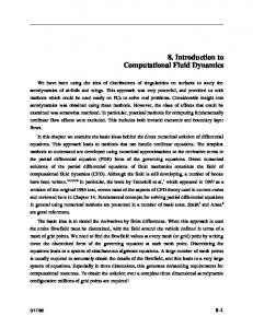
2.1 Föppl/Jeffcott Single Mass Rotor Rotor-dynamic systems have complex dynamics for which analytical solutions are only possible to obtain in the most simple cases. With the computational power that is easily available in modern days, numerical solutions for 2D and even 3D rotordynamic analysis have become the standard. However, these numerical analyses do not provide the deep insight that can be obtained from a step-by-step derivation of an analytical solution, such as how the different system response characteristics are interconnected in the final solution. For example, numerical analysis can accurately estimate the location of the resonance mode of the system, but it cannot give an analytical relationship between that mode frequency and the amount of damping and stiffness on the rotor. The vibration theory for rotor-dynamic systems was first developed by August Föppl (Germany) in 1895 and Henry Homan Jeffcott (England) in 1919 [5]. Employing a simplified rotor/bearing system, they developed the basic theory on prediction and attenuation of rotor vibration. This simplified rotor/bearing system that is commonly known as the Föppl/Jeffcott rotor, or simply the Jeffcott rotor, is often employed to evaluate more complex rotor-dynamic systems in the real world. In this section we overview the analytical derivation of the undamped and damped responses of the Föppl/Jeffcott rotor. We will use these results throughout this chapter to characterize the dynamics of complex rotor-dynamic systems that can be found in actual industrial applications. Figure 2.1 illustrates the single mass Jeffcott rotor with rigid bearings. The rotor disk with mass m is located at the axial center of the shaft. The mass of the shaft in the Jeffcott rotor is assumed to be negligible compared to that of the disk, and thus is considered to be massless during the analysis. The geometric center of the disk C is located at the point (uxC , uyC ) along coordinate axis defined about the bearing center line, and the disk center of mass G is located at (uxG , uyG ). The unbalance eccentricity eu is the vector connecting the points C and G, and it represents the unbalance in the rotor disk. The rotating speed of the disk/shaft is given by ω, and

2.1 Föppl/Jeffcott Single Mass Rotor

19

Fig. 2.1 Single mass Jeffcott rotor on rigid bearings

without loss of generality we assume that eu is parallel with the x-axis at the initial time t = 0. Lastly, uC is the displacement vector with phase angle θ that connects the origin and the point C, and φ is defined to be the angle between the vectors uC and eu . Under the assumption that the rotor disk does not affect the stiffness of the massless shaft, the lateral bending stiffness at the axial center of a simply supported uniform beam is given by 48EI , (2.1) L3 where E is the elastic modulus of the beam, L is the length between the bearings, and I is the shaft area moment of inertia. For a uniform cylindrical shaft with diameter D, the equation for the area moment of inertia is ks =

I=

πD 4 . 64

(2.2)

Additionally, we assume that there is a relatively small effective damping acting on the lateral motion of the disk at the rotor midspan, and the corresponding damping constant is given by cs . This viscous damping is a combination of the shaft structural

20

2


damping, fluid damping due to the flow in turbomachines, and the effective damping added by the bearings. The dynamic equations for the Föppl/Jeffcott rotor are derived by applying Newton’s law of motion to the rotor disk. With the assumption that the shaft is massless, the forces acting on the disk are the inertial force and the stiffness/damping forces generated by the lateral deformation of the shaft. The lateral equations of motion in the x- and y-axes as shown in Fig. 2.1 are found to be mu¨ xG = −ks uxC − cs u˙ xC ,

(2.3a)

mu¨ yG = −ks uyC − cs u˙ yC ,

(2.3b)

where (uxG , uyG ) and (uxC , uyC ) are the coordinates of the mass center and geometric center, respectively. The coordinates of the disk center of mass can be rewritten in terms of its geometric center C and the rotor angle of rotation ωt at time t, uxG = uxC + eu cos(ωt),

(2.4a)

uyG = uyC + eu sin(ωt).

(2.4b)

Substituting the second time derivative of Eqs. (2.4a), (2.4b) into Eqs. (2.3a), (2.3b), we obtain the equations of motion for the Föppl/Jeffcott rotor in terms of the disk geometric center as mu¨ xC + ks uxC + cs u˙ xC = meu ω2 cos(ωt),

(2.5a)

mu¨ yC + ks uyC + cs u˙ yC = meu ω2 sin(ωt).

(2.5b)

We note here that, as the bearings are considered to be infinitely stiff and the rotor disk does not tilt, this model does not include the gyroscopic effects acting on the rotor. The shaft is fixed at the bearing locations, thus it is always aligned to the bearing center line. The effect of the gyroscopic forces in rotor-dynamic systems will be discussed in Sect. 2.2. Additionally, no aerodynamics or fluid-film crosscoupling forces are included in this simplified analysis. These disturbance forces are mostly generated at the seals and impellers of the rotor due to the circumferential difference in the flow, and they are not modeled in this section. Aerodynamic crosscoupling forces will be discussed in Sect. 2.3. As a result of all this, the equations of motion in Eqs. (2.5a), (2.5b) are decoupled in the x- and y-axes.

2.1.1 Undamped Free Vibration The undamped free vibration analysis deals with the rotor vibration in the case of negligible unbalance eccentricity (eu = 0) and damping (cs = 0). The equations of motion in Eqs. (2.5a), (2.5b) are simplified to mu¨ xC + ks uxC = 0,

(2.6a)

mu¨ yC + ks uyC = 0.

(2.6b)


21

The solution to this second order homogeneous system takes the form of uxC = Ax est ,

(2.7a)

uyC = Ay e ,

(2.7b)

st

for some complex constant s. The values of the constants Ax and Ay are obtained from the initial conditions of the rotor disk. Substituting the solution in Eqs. (2.7a), (2.7b) into Eqs. (2.6a), (2.6b) we obtain (2.8a) ms 2 Ax est + ks Ax est = ms 2 + ks Ax est = 0, (2.8b) ms 2 Ax est + ks Ax est = ms 2 + ks Ay est = 0. The above equations hold true for any value of Ax and Ay if the undamped characteristic equation holds, ms 2 + ks = 0.

(2.9)

Solving the above equality for the complex constant s, we obtain the following solution: s1,2 = ±j ωn , where ωn is the undamped natural frequency of the shaft defined as ks 48EI = . ωn = m L3 m

(2.10)

(2.11)

Thus, the solutions to the equation of motion in Eqs. (2.6a), (2.6b), are undamped oscillatory functions with frequency ±ωn . The undamped critical speed of the system is defined as ωcr = ±ωn ,

(2.12)

corresponding to the positive forward +ωn and the negative backward −ωn components. The forward component indicates the lateral vibration that follows the direction of the shaft rotation, and the backward component represents the vibration that moves in the opposite direction. The final solutions to the undamped free vibration are given by the linear combination of the two solutions found in Eqs. (2.7a), (2.7b) and Eq. (2.10), uxC = Ax1 ej ωn t + Ax2 e−j ωn t = Bx1 cos(ωn t) + Bx2 sin(ωn t),

(2.13)

and uyC = Ay1 ej ωn t + Ay2 e−j ωn t = By1 cos(ωn t) + By2 sin(ωn t),

(2.14)

for some values of Axi and Ayi , or Bxi and Byi , which can be found from the initial conditions of the rotor.

22

2


2.1.2 Damped Free Vibration Now consider the free vibration of the Föppl/Jeffcott rotor with a non-zero effective shaft damping acting on the system. Newton’s equation of motion in Eqs. (2.5a), (2.5b) becomes mu¨ xC + ks uxC + cs u˙ xC = 0,

(2.15a)

mu¨ yC + ks uyC + cs u˙ yC = 0.

(2.15b)

The solutions to the above system of homogeneous second order differential equations take the same form as in Eqs. (2.7a), (2.7b). Substituting these solutions into Eqs. (2.15a), (2.15b), we obtain 2 ms + ks + cs Ax est = 0, (2.16a) 2 (2.16b) ms + ks + cs Ay est = 0. These equations hold for any initial condition if the damped characteristic equation holds: ms 2 + ks + cs = 0.

(2.17)

The zeros of the characteristic equation, also know as the damped eigenvalues of the system, are found to be cs ks cs ±j − . (2.18) s1,2 = − 2m m 2m Generally, the rotor/bearing system is underdamped, which means that cs ks < , 2m m and s will have an imaginary component. Define the damping ratio as ζ=

cs . 2mωn

(2.19)

This value corresponds to the ratio of the effective damping cs to the critical value in the damping constant when the system becomes overdamped, or the imaginary part of the solution in Eq. (2.18) vanishes. With this newly defined ratio, the solutions to Eqs. (2.16a), (2.16b) can be rewritten as s1,2 = −ζ ωn ± j ωn 1 − ζ 2 . (2.20) The imaginary component of s1,2 is known as the damped natural frequency, ωd = ωn 1 − ζ 2 . (2.21)


23

For traditional passive bearings, the value of the damping coefficient can vary between 0.3 > ζ > 0.03, although a minimum of ζ = 0.1 is normally considered as needed for the safe operation of the machine. The final solutions to the undamped free vibration are found to be the linear combination of the solutions found in Eqs. (2.7a), (2.7b) and Eq. (2.18), that is, uxC = e−ζ ωn t Ax1 ej ωd t + Ax2 e−j ωd t = e−ζ ωn t Bx1 cos(ωn t) + Bx2 sin(ωn t) , (2.22) and

uyC = e−ζ ωn t Ay1 ej ωd t + Ay2 e−j ωd t = e−ζ ωn t By1 cos(ωn t) + By2 sin(ωn t) ,

(2.23)

for some values of Axi and Ayi , or Bxi and Byi , dependent on the initial condition of the rotor. A typical response for an underdamped system in free vibration is shown in Fig. 2.2. We observe that the response is oscillatory, where the frequency is given by the damped natural frequency ωd . Because of the damping, the magnitude of the oscillation is reduced over time, and the rate of decay is a function of the damping ratio ζ and the undamped natural frequency ωn . For most rotor-dynamic systems, the damping ratio is smaller than 0.3 and the free vibration response is similar to the underdamped response in Fig. 2.2.

2.1.3 Forced Steady State Response Finally, we consider the forced response of the Jeffcott rotor with a non-zero mass eccentricity. Using the definition of ωn and ζ as given above, the equations of motion for the rotor are rewritten into the form u¨ xC + 2ζ ωn u˙ xC + ωn2 uxC = eu ω2 cos(ωt),

(2.24a)

u¨ yC + 2ζ ωn u˙ yC + ωn2 uyC

(2.24b)

= eu ω sin(ωt). 2

In order to simplify the equations of motion, we will combine the x and y displacements of the rotor into the complex coordinates as uC = uxC + j uyC ,

(2.25)

where uC is the displacement of the disk geometric center on the complex coordinate axis. We assume that the steady state solutions of the system of the differential equations in Eqs. (2.24a), (2.24b) are in complex exponential form, uxC = Ux ej ωt ,

(2.26a)

uyC = Uy e

(2.26b)

j ωt

.

24

2


Fig. 2.2 Typical response of an underdamped system in free vibration

It is observed here that, since Eqs. (2.24a), (2.24b) is a linear system with a sinusoidal input of frequency ω, the steady state output solutions will also be sinusoidal signals of the same frequency. Then, the solution of the disk displacement in the complex form is uC = Ux ej ωt + j Uy ej ωt .

(2.27)

Combining the exponential terms in the expression for the above complex rotor displacement, we obtain the solution in the form uC = U ej ωt ,

(2.28)

U = Ux + j Uy .

(2.29)

where

Next, the set of solutions in Eqs. (2.26a), (2.26b) are substituted into Eqs. (2.24a), (2.24b), and the resulting system of equations is 2 −ω + 2j ωζ ωn + ωn2 Ux ej ωt = eu ω2 cos(ωt), (2.30a) 2 (2.30b) −ω + 2j ωζ ωn + ωn2 Uy ej ωt = eu ω2 sin(ωt). The equations for the x-axis and y-axis displacements are combined into the complex form as done in Eq. (2.25) by multiplying Eq. (2.30b) by the complex operator


25

1j , and adding it to the expression in Eq. (2.30a). The resulting complex equation of motion is 2 −ω + 2j ωζ ωn + ωn2 U ej ωt = eu ω2 eωt , (2.31) or

2 −ω + 2j ωζ ωn + ωn2 uC = eu ω2 ,

(2.32)

where eu is the unbalance eccentricity in the complex coordinates as illustrated in Fig. 2.1(b). Considering that the values of both the rotor disk displacement uC and the unbalance eccentricity eu are just complex numbers, we can compute from Eq. (2.32) the ratio between these two complex values as uC fr2 , = eu [1 − fr2 + 2jfr ζ ]

(2.33)

where fr =

ω ωn

(2.34)

is known as the frequency ratio. We notice that right hand side of Eq. (2.33) is not a function of time, and it only depends on the frequency ratio. The complex solution in Eq. (2.33) can be rewritten as the product of a magnitude and a phase shift in the form of |U | −j φ uC = e eu eu =

fr2 e−j φ (1 − fr2 )2 + (2ζfr )2

.

(2.35)

The ratio |U |/eu is known as the dimensionless amplitude ratio of the forced response and is given by |U | |Uy | |Ux | fr2 = = = . eu eu eu (1 − fr2 )2 + (2ζfr )2

(2.36)

The above equation gives the expected amplitude of the rotor vibration as a function of the frequency ratio. Additionally, the angle φ is the phase difference between the uC and eu and is found from Eq. (2.32) to be 2ζfr −1 φ = tan . (2.37) 1 − fr2 The dimensionless amplitude ratio |U |/eu is plotted in Fig. 2.3 over the frequency ratio fr for different values of damping ratio. For very low frequencies, the amplitude ratio is nearly zero since the unbalance forces are small. As the shaft

26

2


Fig. 2.3 Dimensionless amplitude of the forced response for the Jeffcott rotor vs. frequency ratio

speed increases, the amplitude shows a large peak near fr = 1 when ω is near the resonance frequency of the system. The amplitude ratio at the critical speed fr = 1 can be found from Eq. (2.36) to be |U | 1 . = eu 2ζ

(2.38)

When the damping ratio is small, the amplitude ratio increases rapidly near fr = 1 as the unbalance forces excite the rotor resonance mode. For larger values of ζ , the system is nearly critically damped, and only a little of the resonance is seen in the amplitude ratio plot. Finally, for fr 1 the amplitude of vibration approaches 1. The phase angle φ corresponding to different values of the damping ratio is also presented here over a range of frequency ratios in Fig. 2.4. At low frequencies, the phase angle is near zero, and the center of gravity G is aligned with the geometric center of the disk during the rotation of the shaft. When the frequency ratio is near 1 and the shaft speed is close to the natural frequency, we see in Fig. 2.4 that the phase angle is about 90 degrees for all values of damping ratios. This characteristic can be helpful in identifying experimentally the critical speed of actual machines. Lastly, at high frequencies where fr 1, the phase angle approaches 180 degrees. In this case, the center of gravity of the disk is inside the rotor orbit drawn by the rotating path of C, and the unbalance forces work in the opposite direction to the inertial forces of the rotor.

2.2 Rotor Gyroscopic Effects

27

Fig. 2.4 Phase angle φ of the forced response for the Jeffcott rotor vs. frequency ratio

2.2 Rotor Gyroscopic Effects So far, we have found that the rotor lateral dynamics are decoupled in the horizontal and the vertical directions of motion when rigid bearings are assumed. In the Föppl/Jeffcott rotor considered in Sect. 2.1, the shaft axis of rotation was always aligned with the bearing center line, and thus the inertia induced moments acting on the disk were neglected. In this section we investigate how the gyroscopic moments affect the dynamics of the system, as the addition of flexible bearings allows the shaft rotational axis to diverge from the bearing center line. Through an example of a simple cylindrical rotor supported on flexible bearings, the undamped free vibration of the rotor is analyzed, and the natural frequency of the rotor is predicted as a function of the shaft speed. The results will demonstrate the sensitivity of the actual critical speed of rotor-dynamic systems to the geometry and rotating speed of the rotor. The tilt of a rotating shaft relative to the axis of rotation generates gyroscopic disturbance forces. As we will find later in this section, the magnitude of the generated force is proportional to the angle of tilt, angular moment of inertia of the rotor, and the shaft rotational speed. In the modeling and analysis of rotor-dynamic systems, there are two main phenomena that are attributed to the gyroscopic effects. First, the gyroscopic moments tend to couple the dynamics in the two radial direction of motions. A change in the vertical state of the rotor affects the horizontal dynamics,

28

2


Fig. 2.5 Cylindrical rotor with isotropic symmetric flexible bearings [115]

and vice versa. Second, gyroscopic moments cause the critical speeds of the system to drift from their original predictions at zero speed. As we will see later in this section, the gyroscopic moment acting on a rotor can increase or decrease the critical speeds related to some system modes as a function of the rotational speed.

2.2.1 Rigid Circular Rotor on Flexible Undamped Bearings Consider the rigid rotor as shown in Fig. 2.5 with a long cylindrical disk of mass m, length L, and rotating speed ω. The support bearings are considered to be flexible with stiffness coefficients of k1 and k2 in the lateral directions as shown in Fig. 2.5. The axial distance between the bearing location and the rotor center of gravity G is a for the left bearing and b for the right bearing. The total distance between the bearings is Lb . Under the assumption that the shaft has negligible mass, the polar moment of inertia of the uniform rigid cylindrical rotor is given by Jp =

mR 2 , 2

(2.39)

where R is the radius of the rotor. This represents the rotational inertia of the cylinder about its main axis of rotation. The transverse moment of inertia for the same rotor is m 1 R 2 + L2 , (2.40) Jt = 4 3 which represents the rotational inertia about the axis perpendicular to the main axis of rotation. A characteristic of the rotor that will be important in the derivations to follow throughout this section is the ratio P of the polar to the transverse moment


29

of inertia, which is given by P= =

Jp Jt 2 1+

1 L 2 3(R)

.

(2.41)

We notice that the value of this ratio is affected by the geometry of the rotor. For cylindrical rotors where the radius is much larger than the length, or R L, the value of the moment of inertia ratio approaches P ≈ 2. On the other hand, for the case of a long thin rotor with R L, the denominator of Eq. (2.41) approaches infinity and the value of the moment of inertia ratio is approximately P ≈ 0. Finally, the ratio √ in Eq. (2.41) is equal to one if the ratio of the length L to the radius R is equal to 3.

2.2.2 Model of Rigid Circular Rotor with Gyroscopic Moments Consider the rigid cylindrical rotor presented in Fig. 2.5. The lateral displacements of the rotor center of mass are given by xG in the x-direction, and yG in the ydirection. Additionally, the rotation of the rotor at the center of mass G about the x-axis is denoted as θxG , and the equivalent rotation about the y-axis is θyG , as Fig. 2.5 illustrates. The displacements and rotations about the rotor center of mass can be computed as xG =

1 (bx1 + ax2 ), Lb

(2.42a)

yG =

1 (by1 + ay2 ), Lb

(2.42b)

θxG ≈

1 (y2 − y1 ), Lb

(2.42c)

θyG ≈

1 (x2 − x1 ), Lb

(2.42d)

where x1 and y1 are the lateral displacements of the shaft at the first bearing location, as shown in Fig. 2.5. The corresponding displacements at the second bearing location in Fig. 2.5 are given by x2 and y2 . For computing the rotor tilt angle, the approximation sin(θ ) ≈ θ for θ 1 was used. The equations of motion for the translation and rotation of the rotor about its center of mass can be found once again as in Sect. 2.1 through the use of Newton’s law of motion. The resulting equations are mx¨G + αxG − γ θyG = 0,

(2.43a)

my¨G + αyG − γ θxG = 0,

(2.43b)

30

2


Jt θ¨xG + Jp ωθ˙yG + γ xg + δθxG = 0,

(2.43c)

Jt θ¨yG − Jp ωθ˙xG + γ yg + δθyG = 0.

(2.43d)

The defined stiffness parameters in the above equations are α = k1 + k2 ,

(2.44a)

γ = −k1 a + k2 b,

(2.44b)

δ = k1 a + k2 b .

(2.44c)

2

2

The first two equations in Eqs. (2.43a)–(2.43d) describe the lateral translation of the rotor, and the last two equations describes the angular dynamics. The second term in the left-hand side of Eq. (2.43c) and Eq. (2.43d) is the linearized gyroscopic moment about the x- and the y-axes, respectively, for small amplitude motions as discussed in [119]. An important characteristic of the above dynamic equations is that the two equations of translational motion are decoupled from the equations of angular motion when γ is 0, in which case they can be solved separately. The differential equations of Eqs. (2.43a)–(2.43d) are sometimes written in the vector form M X¨ + ωGX˙ + KX = 0, (2.45) where the generalized state vector is given by ⎡ ⎤ xG ⎢ yG ⎥ ⎥ X=⎢ ⎣ θxG ⎦ , θyG

(2.46)

and the mass matrix M, gyroscopic matrix G, and stiffness matrix K are given by ⎡ ⎤ m 0 0 0 ⎢0 m 0 0⎥ ⎥ (2.47) M =⎢ ⎣ 0 0 Jt 0 ⎦ , 0 0 0 Jt ⎡ ⎤ 0 0 0 0 ⎢0 0 0 0⎥ ⎥, (2.48) G=⎢ ⎣0 0 0 Jp ⎦ 0 0 −Jp 0 and

⎡

α ⎢0 K =⎢ ⎣0 γ respectively.

0 α γ 0

0 γ δ 0

⎤ γ 0⎥ ⎥, 0⎦ δ

(2.49)


31

We notice here that the mass matrix is always diagonal, and the stiffness matrix is diagonal when γ is zero. On the other hand, the gyroscopic matrix is skew symmetric, and it represents the coupling between the motions in the x- and the y-axes. This is one of the main characteristics of the gyroscopic effects as mentioned at the beginning of this section. For the remainder of this section, we will make the simplifying assumption that the stiffnesses of all support bearings are the same, k = k 1 = k2 , and that the rotor is axially symmetric about its center of mass, Lb = a = b. 2 This provides the decoupling condition of γ = 0 for the rotor equations of motion in the translational and the angular direction in Eqs. (2.43a)–(2.43d). In this case, the system stiffness matrix becomes ⎡ ⎤ α 0 0 0 ⎢ 0 α 0 0⎥ ⎥ K =⎢ (2.50) ⎣ 0 0 δ 0⎦. 0 0 0 δ

2.2.3 Undamped Natural Frequencies of the Cylindrical Mode Here we are to solve the rotor equations given in Eq. (2.43a) and Eq. (2.43b) corresponding to the rotor translational or parallel motion. Using the methods as in Sect. 2.1, we assume that the system of homogeneous linear differential equations has solutions in the complex exponential form xG = UxG est ,

(2.51a)

yG = UyG est ,

(2.51b)

for some constant values of UxG and UyG . Substituting these solutions into Eq. (2.43a) and Eq. (2.43b), we rewrite the equations of motion as 2 ms + α UxG = 0, (2.52a) 2 (2.52b) ms + α UyG = 0. The expression within the parentheses on the left-hand sides of the above two equations is known as the characteristic polynomial. We know from Sect. 2.1 that the zeros of the characteristic equation, ms 2 + α = 0,

(2.53)

32

2


are the eigenvalues of the system corresponding to the cylindrical mode. The characteristic equations for the horizontal x- and the vertical y-axes of motion given above are identical and decoupled. This is expected since the lateral translation does not cause rotor tilt, and the corresponding gyroscopic moment is zero. The natural frequency ωn corresponding to the rotor parallel vibration is found from the zeros of the characteristic equation in Eq. (2.53). More precisely, the imaginary components of the zeros give the natural frequency s = ±j ωn .

(2.54)

In the case of the cylindrical mode, the horizontal undamped natural frequency has the forward mode ωn1 and the backward mode ωn2 . The undamped natural frequency in the vertical direction has the forward mode ωn3 and the backward mode ωn2 . These natural frequencies are found to be ωn1 = ωn3 = 2k/m, (2.55a) ωn2 = ωn4 = − 2k/m. (2.55b)

2.2.4 Undamped Natural Frequencies of the Conical Mode We now consider the angular dynamics of the rotor, given in Eq. (2.43d) and Eq. (2.43c). We will assume once again that the solutions to the homogeneous system of differential equations take the form θxG = ΘxG est ,

(2.56a)

θyG = ΘyG e ,

(2.56b)

st

for some constant values of ΘxG and ΘyG . Substituting these solutions into Eq. (2.43c) and Eq. (2.43d), we obtain the following system of homogeneous equations: 2 Jt s + δ ΘxG + Jp ωsΘyG = 0, (2.57a) 2 (2.57b) Jt s + δ ΘyG − Jp ωsΘxG = 0. The characteristic equation for the above system is 2 Jt s + δ Jp ωs det = 0. −Jp ωs Jt s 2 + δ

(2.58)

The angular dynamics about the different lateral axes of motion are coupled through the terms corresponding to the gyroscopic moment in the above characteristic equation. In the remainder of this section, we will discuss how the rotating speed of the shaft, and thus the gyroscopic moment acting on the rotor, affects the natural frequencies of the conical mode.


33

2.2.4.1 Conical Mode at Zero Rotating Speed For the special case where the rotational speed is zero (ω = 0), the characteristic equation in Eq. (2.58) becomes decoupled in the x- and the y-axes. The conical natural frequencies for the non-rotating rotor can be found by solving for the zeros of the undamped characteristic equation in Eq. (2.58), kL2b s = ±j . (2.59) 2Jt The resulting non-rotating conical natural frequency is kL2b ωnC0 = . 2Jt

(2.60)

The non-rotating conical natural frequency ωnC0 will appear again in the calculation of the rotor conical mode with non-zero rotating speed.

2.2.4.2 Conical Mode at Zero Rotating Speed In the general case with non-zero rotating speed (ω = 0), the characteristic equation, after expanding the determinant of the matrix in Eq. (2.58), becomes 2 2 Jt s + δ + (Jp ωs)2 = 0.

(2.61)

In the same way as in Sect. 2.1, the undamped conical natural frequency ωnC is found from the complex zeros of the characteristic equation in Eq. (2.61), s = ±j ωnC . This is an expression equivalent to 2 s 2 = −ωnC .

Replacing the above expressions for s in the characteristic equation in Eq. (2.61), we obtain 2 2 −Jt ωnC + δ − (Jp ωωnC )2 = 0. (2.62) Factoring the above expression into two terms gives 2 2 Jt ωnC − δ + Jp ωωnC Jt ωnC − δ − Jp ωωnC = 0.

(2.63)

This equation is further simplified by dividing both sides of the above equality by Jt , and substituting in the derived expression for the moment of inertia ratio P and the

34

2


non-rotating conical natural frequency ωnC0 . The resulting characteristic equation is 2 2 2 2 (2.64) + P ωωnC ωnC − ωnC0 − P ωωnC = 0. ωnC − ωnC0 Next, we define the dimensionless conical mode natural frequency ratio ω¯ nC and the dimensionless conical mode frequency ratio frC0 as ω¯ nC =

ωnC , ωnC0

(2.65)

frC0 =

ω , ωnC0

(2.66)

and

respectively. Then, by dividing both sides of Eq. (2.64) by the square of ωnC0 , and substituting in the non-dimensional parameters defined in Eqs. (2.65) and (2.66), we obtain 2 2 ω¯ nC + PfrC0 ω¯ nC − 1 ω¯ nC − PfrC0 ω¯ nC − 1 = 0. (2.67) The natural frequencies of the conical modes are the four zeros of Eq. (2.67). Here we organize these modes as the lower modes and the higher modes. The zeros of the first term in Eq. (2.67) provide frequencies corresponding to the forward component of the non-dimensional lower mode ω¯ n3 , and the backward component of the non-dimensional higher mode ω¯ n8 as ω¯ n5 = −PfrC0 /2 + (PfrC0 /2)2 + 1 > 0, (2.68a) (2.68b) ω¯ n8 = −PfrC0 /2 − (PfrC0 /2)2 + 1 < 0. On the other hand, the zeros of the second term in Eq. (2.67) provide frequencies corresponding to the backward component of the non-dimensional lower mode ω¯ n6 , and the forward component of the non-dimensional higher mode ω¯ n7 as (2.69a) ω¯ n6 = PfrC0 /2 − (PfrC0 /2)2 + 1 < 0, (2.69b) ω¯ n7 = PfrC0 /2 + (PfrC0 /2)2 + 1 > 0. The forward and backward conical modes are plotted in Fig. 2.6 over the frequency ratio frC0 and for different values of P . The dashed line in the figures connects the points where the rotor speed matches the frequency of the mode at the corresponding frequency ratio, and the system is in the condition of resonance. Figure 2.6 shows how the gyroscopics effects acting on the rotor causes the natural frequency of the system to drift. For long rotors where P ≈ 0, the gyroscopic moment is small, and the frequency of the conical mode remains unaffected to the rotational speed and frC0 . As the value of P increases for different geometries of the rotor, we can observe a more significant drift in the mode frequency. For example,


35

Fig. 2.6 Dimensionless conical natural frequency ratio versus the conical mode frequency ratio

36

2


for the extreme case of P ≥ 1, we observe in Fig. 2.6 that the shaft rotation would never excite one of the forward conical modes as the gyroscopic effects keep the mode frequency always above the rotor operating speed.

2.3 Instability due to Aerodynamic Cross Coupling Cross-coupling forces are in many cases the main cause of instability in rotordynamic systems. These forces are generated in components such as fluid-film bearings, impellers and seals, which are essential for the operation of the turbomachines. The aerodynamic cross-coupling forces are generated by the flow difference in the uneven clearances around impellers and seals caused by the rotor lateral motion. Machines with traditional fluid-film bearings are sometimes more vulnerable to these effects, as the rotor is not centered in the clearance and it is susceptible to go into the whirling motion. It is common for cross-coupling disturbance forces to generate large rotor vibration, and eventually drive the machine to instability. In this section we focus on the aerodynamic cross-couple stiffness generated by the flow of gas through the impeller and seal clearances. A commonly observed effect of the cross-coupling forces is the rapid loss of damping in the rotor/bearing system modes, particularly the forward mode corresponding to the first critical speed. This results in large subsynchronous rotor vibrations, as the cross-coupling forces increase together with the pressure build-up in the compressor or pump. Eventually, the system mode loses all its damping for large enough magnitudes of the cross-coupling forces, and the rotor-dynamic system becomes unstable. The destabilizing effects of the aerodynamic cross-coupling forces are amplified when they are generated near the rotor midspan, far from the supporting bearings, where the effectiveness of the added damping by the bearings is significantly reduced.

2.3.1 Aerodynamic Cross Coupling in Turbines J.S. Alford in 1965 studied the forces found in the clearances around the aircraft gas turbine engine rotors, which tend to drive the turbine wheel unstable [3, 30]. These forces, affecting both turbines and compressors, came to be known as Alford forces or aerodynamic cross-coupling forces. The aerodynamic cross-coupling forces are normally expressed in terms of stiffness values, connecting the two axes of the rotor lateral motion. Define the rotor lateral axes of motion as shown in Fig. 2.1. Given that the rotor x and y displacements at the location of a turbine stage along the rotor length are denoted by xd and yd , the cross-coupling forces acting on the turbine rotor take the form qsxx qsxy xd Fdx = , (2.70) Fdy qsyx qsyy yd

2.3 Instability due to Aerodynamic Cross Coupling

37

where Fdx and Fdy are the x-axis and y-axis components of the resulting crosscoupling forces, respectively. The coefficients qsxx and qsyy are related to the principal (direct) aerodynamic stiffness, and qsxy and qsyx are known as the cross-coupling aerodynamic stiffness coefficients. It is normally the case in actual machines that the principal aerodynamic stiffness coefficients are negligible when compared to the cross-coupling coefficients, and −qsxy = qsyx . Then, the expression for the cross-coupling forces can be simplified to the form xd Fsx 0 −qa = , (2.71) Fsy qa 0 yd for some cross-coupling stiffness coefficient qa . A simple estimate of the crosscoupling aerodynamic stiffness coefficient for one turbine stage was introduced by Alford in his derivation as Tβ qa = , (2.72) D m Lt where T is the torque on the turbine stage, β is a correction constant, Dm is the mean blade diameter, and Lt is the turbine blade radial length. Based upon his experience with aircraft gas turbines, Alford suggested the value of this constant to be 1.0 < β < 1.5.

2.3.2 Aerodynamic Cross Coupling in Compressors In the case of compressors, the impellers are subject to the same cross-coupling stiffness as presented in Eq. (2.71) for a single turbine stage. In industrial compressor applications, a common range for the value of the impeller aerodynamic cross-coupling coefficient per each stage or impeller is 175,000 N/m ≥ qa ≥ 525,000 N/m.

(2.73)

In the rotor-dynamic analysis of compressors, the rotor vibration level and stability are often evaluated at the average cross-coupling stiffness coefficient value of qa = 350,000 N/m per impeller stage [5]. Moreover, a common rule for compressors that is also based on experience is that the cross-coupling stiffness contribution of the end impellers in multi-stage machines is negligible and not counted when computing the total cross-coupling stiffness of compressors. Seals are employed in compressors and other turbomachines to prevent the gas leakage between the different machine stages. The compressible flow in these seals generate lateral forces that act on the rotor in the form of stiffness and damping, Fsx ksxx ksxy xd csxx csxy x˙d = + , (2.74) Fsy ksyx ksyy yd csyx csyy y˙d

38

2


where Fsx and Fsx are the x and y components of the cross-coupling forces generated by the seals, respectively. Once again, the principal stiffness coefficients and the damping terms are relatively small when compared to the cross-coupling stiffness coefficients, and are usually taken to be equal to zero. Thus, the equation for the seal cross-coupling forces is often simplified to xd 0 ksxy Fsx = , (2.75) Fsy ksyx 0 yd where ksxy < 0 and ksyx > 0 are known as the seal cross-coupling stiffness coefficients. Finally, the total aerodynamic cross coupling for compressors is sometimes estimated based on the horsepower of the machine. This approximation is given as Qa =

63,000(HP)β . DhN

(2.76)

The parameters of the above expression are the compressor horsepower HP, the impeller diameter D (in), the dimension of the most restrictive flow path h (in) and the shaft rotating speed N (rpm). A common value of the correction constant introduced by Alford is β = 1.0 based upon experience [5]. The total cross-coupling stiffness is given in the English unit of lbf/in and can be converted into the equivalent SI unit N/m by a factor of 175. An expression similar to Eq. (2.76) is employed by the API to predict the applied aerodynamic cross-coupling stiffness in the stability analysis for compressors. This expression will be discussed below in Sect. 2.4.

2.4 Rotor-Dynamic Specifications for Compressors Turbomachines such as compressors play an integral role in the manufacturing processes of the chemical and petrochemical industries. Therefore, each machine is carefully audited before being commissioned in order to guarantee that it meets the performance and reliability standards agreed to be needed for continuous operation. Both the International Organization for Standardization (ISO) and the American Petroleum Institute (API) published sets of specifications developed for different types of turbomachine used in industrial applications, although the API standards are largely preferred in the chemical and petrochemical industries. A list of those API standards relevant to different types of turbomachine are presented in Table 2.1. In this section we present a brief summary of the different lateral rotor-dynamic analyses that are required by the API specifications for compressors. These analyses guide compressor end-users, original equipment manufacturers (OEM), component manufacturers, service companies and educational institutions on proper design, manufacturing and on-site installation of machines. For a more detailed description of the required analyses for compressors, please refer to the original API Standard 617 [6].

2.4 Rotor-Dynamic Specifications for Compressors Table 2.1 API Specification for Compressors, Fans and Pumps [111]

39

API standard number

Machine type

610

Centrifugal pumps

612

Steam turbines

617

Axial and centrifugal compressors

673

Centrifugal fans

2.4.1 Lateral Vibration Analysis The API defines the critical speed to be the rotational speed of the shaft that causes the rotor/bearing/support system to operate in a state of resonance. In other words, the frequency of the periodic excitation forces generated by the rotor operating at the critical speed coincides with the natural frequency of the rotor/bearing/support system. Generally, the lateral critical speed is the most relevant, and it is given by the natural frequency of rotor lateral vibration interacting with the stiffness and damping of the bearings. In the present day, it has become common for high performance machines to operate above the first critical speed, but the continuous operation at or near the natural frequencies is generally not recommended. Figure 2.7 illustrates the lateral vibration amplitude versus the rotating speed for a typical rotor-dynamic system. The basic characteristics of the vibration response that API employs to evaluate the machine are identified in the figure. The ith critical speed is denoted as Nci , which is located at the ith peak in the vibration response plot with amplitude of Aci . The amplification factor of a critical speed is defined as the ratio of the critical speed to the difference between the initial and final speed above the half-power of the peak amplitude N1 − N2 , as shown in Fig. 2.7. Lastly, the maximum continuous operating speed (MCOS) of the system corresponds to the 105 % of the highest rated speed of the machine in consideration, and the speeds between the MCOS and the minimum operating speed of the machine is known as the operating speed range. The effective damping at a particular critical speed in a rotor-dynamic system is measured through the amplification factor, AF =

Nc1 . N 2 − N1

(2.77)

The measurement of the amplification factor is illustrated in Fig. 2.7 for the first critical speed. A large amplification factor corresponds to a steep resonance peak with low damping. Therefore, a small value of AF is desired for modes within or near the operating speed range of the machine. For modes with large amplification factors, a minimum separation margin SM is required between the corresponding critical speed and the operating speed range of the machine. The critical speeds of the rotor/support system can be excited by periodic disturbance forces that need to be considered in the design of the machine. The API identifies some of the sources for these periodic disturbances to be [6]:

40

2

Nci Nmc

= =

N1 , N2 AF

= = = = =

SM Aci


Rotor ith critical speed (rpm). Maximum continuous operating speed MCOS (105 % of highest rate speed). Initial and final speed at 0.707 × peak amplitude. Amplification factor. Nc1 N2 −N1 . Separation margin. Amplitude at Nci .

Fig. 2.7 Example of a rotor forced response [6]

• • • • • • • • • • • • •

rotor unbalance, oil film instabilities, internal rub, blade, vane, nozzle, and diffuser passing frequencies, gear tooth meshing and side bands, coupling misalignment, loose rotor components, hysteretic and friction whirl, boundary layer flow separation, acoustic and aerodynamic cross-coupling forces, asynchronous whirl, ball and race frequency of rolling-element bearings, and electrical line frequency.

2.4 Rotor-Dynamic Specifications for Compressors

41

Fig. 2.8 Undamped critical speed vs. stiffness map [6]

Many of these disturbances are related to the mechanical and electrical characteristics of the machine hardware and they can be corrected at the design stage or through proper maintenance. For the lateral vibration analysis, we focus on the forced response due to the rotor unbalance. The cross-coupling forces will be discussed in the rotor stability analysis later in this section.

2.4.1.1 Undamped Critical Speed Analysis Estimating the critical speeds and the mode shapes of the rotor-dynamic system between zero and 125 % of the MCOS is generally the first step in the lateral analysis. The critical speeds of the rotor/support system are estimated from the undamped critical speed map, superimposed by the calculated system support stiffness in the horizontal direction (kxx ) and the vertical direction (kyy ) as shown in Fig. 2.8. A quick estimate of a particular critical speed can be found from the figure at the intersection of the corresponding curve in the critical speed map and the bearing stiffness curve. The actual locations of the critical speeds of the system below the MCOS should be validated in a test stand as required by the API standard [6]. Mode shape plots for the relevant critical speeds should also be included in this initial analysis.

42

2


2.4.1.2 Damped Unbalance Response Analysis A damped unbalance or forced response analysis including all the major components of the rotor/bearing/support system is required by the API standard to be included in the machine audit. The critical speed and the corresponding amplification factor are identified here for all modes below 125 % of the MCOS. The proper level of unbalance in compressor rotors for the forced response test is specified in the SI units to be 4 × Ub , where Ub = 6350

W . N

(2.78)

The two parameters in the above definition is the journal static load W (kg), and the maximum continuous operating speed N (rpm). The journal load value used for W and the placement of the unbalance along the rotor are determined by the mode to be excited as illustrated in Fig. 2.9. For example, to excite the first bending mode, the unbalance is placed at the location of the maximum deflection near the rotor midspan, and W is the sum of the static loads at both support bearings. Figure 2.9 applies to machines with between-bearing and overhung rotors as given in [6]. Based on the results from the forced response, a separation margin is required for each mode below the MCOS that presents an amplification factor equal to or greater than 2.5. The required minimum separation margin between the mode critical speed and the operating speed range is given as 1 SM = min 17 1 − , 16 . (2.79) AF − 1.5 On the other hand, if the mode with an amplification factor equal to or greater than 2.5 is above the MCOS, then the requirement for the minimum separation margin between the mode critical speed and the machine MCOS is specified to be 1 SM = min 10 + 17 1 − , 26 . (2.80) AF − 1.5 The requirements on the separation margin is employed to determine an operating speed of the machine that avoids any critical speed with the potential to damage the system. Finally, for traditional fluid-film and rolling-element bearings, the peak-to-peak amplitude limit of the rotor vibration is given by 12,000 A1 = 25 , (2.81) N where N is the maximum continuous operating speed in rpm. At the same time, the peak amplitude of the rotor vibration at any speed between zero and Nmc should not exceed 75 % of the minimum machine clearance. We will later see in Chap. 7 that this particular specification generally does not apply to systems with active magnetic bearings.


43

Fig. 2.9 Unbalance values and placements as specified by API [6]

2.4.2 Rotor Stability Analysis As the name indicates, this analysis investigates the stability of the rotor-dynamic system in the presence of common destabilizing forces that compressors and turbines are subjected to during normal operation. The dominant forces in this group are often the aerodynamic cross-coupling forces, which were introduced in Sect. 2.3. The stability analysis is required by the API for compressors and radial flow rotors with the first rotor bending mode below the MCOS [6]. The stability of the rotor-dynamic system in the API standard is normally evaluated by the amount of damping on the first forward mode. The standard measure of mechanical damping employed in the API standard is the logarithmic decrement, which is computed as the natural logarithm of the ratio between the amplitudes of two successive peaks. The relation between the mode logarithmic decrement δ and

44

2


the corresponding damping ratio ζ can be found to be δ=

2πζ 1 − ζ2

.

(2.82)

2.4.2.1 Level I Stability Analysis The Level I stability analysis is the first step of the stability analysis. It is intended to be an initial screening to identify the machines that can be considered safe for operation. The inlet and discharge conditions for the stability analysis are selected to be at the rated condition of the machine, although it is allowed for the vendor and the purchaser to agree on a different operating condition to perform the test. The predicted cross-coupling stiffness in kN/mm at each stage of a centrifugal compressor is given by qA = HP

Bc Cρd , Dc Hc Nρs

(2.83)

and that of an axial compressor is given by qA = HP

Bt C . Dt Ht N

(2.84)

The parameters in the above equations are HP Bc Bt C Dc , Dt Hc Ht N ρd ρs

= = = = = = = = = =

rated compressor horsepower, 3, 1.5, 9.55, impeller diameter (mm), minimum of diffuser or impeller discharge width (mm), effective blade height (mm), operating speed (rpm), discharge gas density per impeller/stage (kg/m3 ), and suction gas density per impeller/stage (kg/m3 ).

The predicted total cross-coupling stiffness QA is the sum of the qA for all the impellers/stages in the compressor. In the Level I analysis, the stability of the rotor-dynamic system is tested for a varying amount of the total cross-coupling stiffness. The applied cross-coupling stiffness value ranges from zero to the smallest between 10QA and the maximum cross-coupling stiffness before the system becomes unstable. This point of instability is identified by the API to correspond to the cross-coupling stiffness value Q0 where the damping, or logarithmic decrement of the system first forward mode becomes zero. For the Level I analysis, the cross-coupling stiffness is assumed to be concentrated at the rotor mid-span for between-bearing machines, or at the center of mass of each impeller/stage for cantilevered systems.


45

Fig. 2.10 Typical plot of logarithmic decrement corresponding to the first forward mode vs. applied cross-coupling stiffness for Level I stability analysis

An important graph that is required by the API to be included in the Level I analysis is the plot of the logarithmic decrement δ for the first forward mode versus the applied cross-coupling stiffness Q, as presented in Fig. 2.10. The predicted total cross-couple stiffness QA and the corresponding logarithmic decrement of the first forward mode δA are marked in the figure. Additionally, Q0 corresponds to the cross-coupling stiffness when the logarithmic decrement of the first forward mode becomes zero. The boundary at δ = 0.1 corresponds to the pass/fail condition of the stability analysis, which will be discussed later in this section. We note here that, although with traditional passive bearings the first forward mode is generally the first one to be driven to instability by the cross-coupling stiffness, the situation is not as straightforward with AMBs. As the active controller in these magnetic bearings normally has a direct influence on any system mode within the controller bandwidth, the interaction between the controller and the crosscoupling effects has the potential to destabilize a group of modes within and above the compressor operating speed range. Therefore, the logarithmic decrement of all modes within the levitation controller bandwidth is sometimes inspected during the Level I stability analysis for machines with magnetic bearings. Based on the results from the Level I stability analysis, machines that do not meet certain stability criteria are required to undergo a more advanced Level II stability analysis. For centrifugal compressors, a Level II stability analysis is required

46

2


if either of Q0 /QA < 2, δA < 0.1,

(2.85a) (2.85b)

is found to be true. In the case of axial compressors, a Level II analysis is required only if δA < 0.1.

(2.86)

2.4.2.2 Level II Stability Analysis The Level II stability analysis is a complete evaluation of the rotor/bearing system with the dynamics of all the compressor components generating the aerodynamic cross-coupling stiffness or affecting the stability of the overall machine. Some of these components are [6] • • • • •

seals, balance piston, impeller/blade flow, shrink fit, and shaft material hysteresis.

Details on the methodology of the analysis is left to a great extent to be decided based on the latest capabilities of the vendor. API does not specify how each dynamic component is handled in the analysis. The operating condition of the machine used in the analysis is the same as in the Level I analysis. During the Level II analysis, the API requires the vendor to initially identify the frequency and logarithmic decrement of the first forward damped mode for the bare rotor/support system. Then, the analysis is repeated after adding the dynamics of each component previously identified to affect the stability of the rotor-dynamic system. Finally, the frequency and logarithmic decrement δf of the first damped forward mode is computed for the total assembled system. The pass/fail condition of the Level II stability analysis stated by API 617 is δf > 0.1.

(2.87)

If this is satisfied, then the machine is considered to have guaranteed stability in the rated operating condition. On the other hand, if the pass/fail condition cannot be satisfied, API allows the vendor and purchaser to mutually agree on an acceptable level of δf considered to be sufficient for the safe operation of the machine. Finally, it is recognized in the API 617 that other analysis methods exist for evaluating the stability of rotor-dynamic systems, and these methods are constantly being updated. Therefore, it is recommended to follow the vendor’s stability analysis methods if the vendor can demonstrate that these methods can successfully predict a stable rotor.

2.5 Rotor Finite Element Modeling

47

2.5 Rotor Finite Element Modeling The first priority of the bearings in a rotor-dynamic system is commonly the support of the rotor lateral dynamics. Although the rotor axial vibrations also need to be carefully analyzed for possible signs of trouble, the main source of rotor instability in most rotating machines comes from the lateral or radial vibrations. For this reason, an accurate model of the system lateral dynamics is essential for the analysis and simulation testing that are required during the design and commissioning phases of these machines. In the case of systems with AMBs, the need for an accurate model is even higher as the unstable bearing system requires reliable model-based rotor levitation controllers for normal operation. The lateral dynamics of flexible rotors are described by partial differential equations. These are complex equations with spatially distributed parameters, and it usually is not possible to derive analytic solutions for rotors with complex geometries. In real world applications, a linearized approximation model of the rotor lateral dynamics is normally sufficient for analyzing rotor-dynamic systems and designing rotor levitation controllers for AMBs. Such a model can be obtained by means of the finite element method (FEM), where the description of the spatially continuous rotor is simplified to the degrees of freedom corresponding to a finite number of shaft elements, effectively eliminating the spatial variable in the original beam equation [119]. In this section we present a brief summary of the process for obtaining the twodimensional finite element model of a rotor-dynamic system. Detailed step-by-step description of the finite element method can be found in the many available finite element textbooks such as [4], and the application of this method for modeling the rotor-dynamic system is thoroughly discussed in [5] and [119]. In this section, we only present a concise description of the process for deriving the finite element model, as an introduction to what will later be used in Chap. 7 for the synthesis of the AMB lateral levitation controller.

2.5.1 Discretizing Rotor into Finite Elements As the first step of deriving a finite element model, the rotor is axially divided into simple uniform beam elements connecting two adjacent node points. A typical mesh of a simple rotor is illustrated in Fig. 2.11, where the node points are shown as dark dots. The selection of an adequate rotor mesh must follow some rules that are based on the rotor geometry, as well as the locations of the rotor disks, bearings, and other rotor-dynamic components. First, a nodal point must be placed at each location along the rotor with a step change in the diameter, so that all shaft elements have a uniform radius. This will later simplify the modeling of the dynamics for each individual shaft element. Second, a node point is defined at each location with a mass/inertia disk, bearing, seal, and any other source of external disturbance force. By the same token, all sensor locations and other measurement points are also collocated with the shaft node points. This rule simplifies the definition of the input and

48

2


Fig. 2.11 Rotor mesh example

Fig. 2.12 Beam element and generalized displacements of nodes i and i + 1

output variables in the final expression of the finite element model. Finally, the ratio of the element’s length to diameter must be about one or less in order to guarantee the accuracy of the finite element formulation. The rotor shown in Fig. 2.11 has a total of 17 elements and 18 node points. It is common for the elements and nodes to be numbered from left to right, as demonstrated in the figure. The support bearings, with given stiffness and damping coefficients, are located in this example at the nodes 4 and 15. For the remaining of this section, we will assume that the general rotor mesh considered here is composed of n beam elements, corresponding to a total of n + 1 node points

2.5.2 Approximating Element Displacement Functions and Nodal Displacement Once the shaft is sectioned into smaller elements, the dynamics of each shaft section is studied independently. The generalized displacements and rotations of the shaft element are described through the degrees of freedom that are defined at each node point. The degrees of freedom for a typical beam element are shown in Fig. 2.12. Considering only the lateral dynamics of the rotor for simplicity, each shaft section has eight degrees of freedom, corresponding to the two displacements and two rotations about the lateral axes at each node point. As shown in Fig. 2.12, the lateral displacements of the ith node are given as uxi in the horizontal x-axis, and uyi in the vertical y-axis. The angular displacements at the same node about the y- and x-axes are defined, respectively, as ∂ux , ∂z ∂uy . θx = ∂z

θy =

(2.88a) (2.88b)


49

The degrees of freedom of the ith node point are collected in the generalized displacement vector qi , which describes the position and rotation of the node at a given time. The displacement and rotation variables are sorted in the mentioned vector as ⎡ ⎤ uxi ⎢ uyi ⎥ ⎥ (2.89) qi = ⎢ ⎣ θyi ⎦ . θxi Lastly, the generalized displacement of the ith shaft element illustrated in Fig. 2.12 combines the generalized displacement vectors at the end nodes qi and qi+1 . The generalized displacement vector for the ith element in Fig. 2.12 is defined as qi Qi = . (2.90) qi+1 The generalized displacement vector defined above is used in the derivation of the dynamic model to estimate the state of the entire shaft section. Thus, the eight variables in Qi uniquely describe the shape of the ith beam element in the finite element formulation. Based on the degrees of freedom defined at a shaft element of the rotor mesh, the lateral translation and rotation is interpolated at any arbitrary point along the shaft element. The shape of the entire shaft element is estimated in terms of the generalized displacement vector Qi and the shape functions Ni . The shape functions that form a third order polynomial basis of the shaft element are given as [4] 1 3 L − 3z2 L + 2z3 , 3 L 1 N2 = 2 zL2 − 2z2 L + z3 , L 1 N3 = 3 3z2 L − 2z3 , L 1 N4 = 2 −z2 L + z3 . L

N1 =

(2.91a) (2.91b) (2.91c) (2.91d)

The parameter L is the length of the shaft element, and the variable z is the axial position along the element’s length. The above shape functions are illustrated in Fig. 2.13. For the given basis of shape functions in Eqs. (2.91a)–(2.91d), the generalized lateral translation of the ith shaft element at an arbitrary axial position z is expressed as a function of the time t and the axial offset from the leftmost node as uxi (z, t) N 1 0 N2 0 N3 0 N4 0 = (2.92) Qi . uxi (z, t) 0 N1 0 −N2 0 N3 0 −N4 In the same way, the lateral rotations θyi (z, t) and θxi (z, t) at an arbitrary axial position z can be found by computing the partial derivative of Eq. (2.92) with respect

50

2


Fig. 2.13 Element Hermite shape function

to the axial offset z as shown in Eqs. (2.88a), (2.88b). An important observation from the expressions in Eq. (2.92) is that the spatial variable z is contained in the matrix of basis functions in Eq. (2.92), while only the generalized displacement vector Qi is a function of time. Thus, the description of the dynamics of the original continuous shaft element is simplified in the finite element formulation into a finite number of degrees of freedom corresponding to a discrete shaft [119].

2.5.3 Formulating Equations of Motion for Each Element The equation of motion for the ith shaft element is determined following the Lagrange formulation: ∂Ri d ∂Li ∂Li + = 0. (2.93) − dt ∂ q˙i ∂qi ∂ q˙i


51

The Lagrangian of the ith element Li is defined as the difference between the element’s kinetic energy Ti and potential energy Ui , Li = Ti − Ui .

(2.94)

Additionally, Ri captures the energy dissipation in the system due to the internal friction or damping, and it is known as the dissipation function. Given that the generalized displacement of a shaft element is approximated as shown in Eq. (2.92), the terms for both the kinetic and potential energies can be easily found based on either the Bernoulli–Euler or the Timoshenko beam theories [4]. For each of the beam elements, the potential energy comes mainly from the beam bending and shear effects. On the other hand, the level of the kinetic energy is determined by both the lateral and the rotatory inertial effects in the shaft element. By expanding the Lagrange equation in Eq. (2.93) with the energy formulation for the individual shaft section, an expression describing the lateral dynamics of the ith element of the rotor mesh is obtained in the form of the vector differential equation, ¨ i + C Q˙ i + Gi Q ˙ i + Ki qi = Fi . Mi Q

(2.95)

The system matrices are the mass matrix Mi , gyroscopics matrix Gi , stiffness matrix Ki , and the damping matrix Ci . The generalized external force vector Fi is added to the Lagrange equation to account for the external forces and torques perturbing the system. The objective of the finite element formulation is to find the expressions for the system matrices, based on Eq. (2.93) and the generalized displacements in Eq. (2.92).

2.5.4 Element Mass and Gyroscopic Matrices The kinetic energy of a mesh element comes from the translational and angular momentum of the shaft. For a uniform ith beam element with the generalized displacement as defined by Eq. (2.92), the resulting expression of the kinetic energy takes the form 1 ˙T 1 ˙T ˙ Ti = Q (2.96) i Mi Qi + ωQi Wi Qi . 2 2 The matrix Mi corresponds to the mass matrix of the shaft element, and the matrix Wi is related to the polar moment of inertia of the element with a rotational speed of ω. A detailed step-by-step description of how to determine the expressions for these matrices can be found in [5] and [119]. The contribution of the kinetic energy in the Lagrange equation appears in the first and second terms of Eq. (2.93). The first term of the Lagrange equation in Eq. (2.93) with the above form of the kinetic energy is given by d ∂T ¨ i + 1 ωWI Q˙ i . (2.97) = Mi Q dt ∂ Q˙ i 2

52

2


The corresponding second term of the Lagrange equation is −

1 ∂T = − ωWiT Q˙ i . ∂Qi 2

(2.98)

Combining the two terms of the kinetic energy in the Lagrange equation, we obtain the equation ∂T d ∂T ¨ i + 1 ω Wi − WiT Q˙ i , = Mi Q − dt ∂ Q˙ i ∂Qi 2 ¨ i + Gi Q ˙ i, = Mi Q

(2.99)

where the gyroscopic matrix Gi is defined above in terms of the matrix Wi and the rotor speed ω. The final expressions of the mass matrix Mi and the gyroscopic matrix Gi for a uniform shaft element can be found in [5] and [119]. These matrices are expressed in terms of the element’s length, cross sectional area, and material density. Therefore, as the expressions are identical for all elements in the mesh, it is relatively simple to automate the process of finding these matrices for all shaft sections, given that the rotor mesh has been selected according to the rules described at the beginning of this section.

2.5.5 Element Stiffness Matrix Based on the Bernoulli–Euler beam theory, the potential energy of a uniform shaft element comes from the internal strain energy due to the lateral bending. For the ith uniform beam element with the generalized displacements uxi (z, t) and uxi (z, t) defined as in Eq. (2.92), the resulting expression of the potential energy takes the quadratic form 1 (2.100) Ui = QTi Ki Qi . 2 The matrix Ki is the stiffness matrix. It describes the axial strain/stress due to the lateral bending of the beam element. A detailed derivation of the potential energy term Ui and the stiffness matrix can be found in [5] and [119]. Substituting the above expression of the potential energy to the second term of the Lagrange equation in Eq. (2.93), we obtain ∂Ui = Ki Qi . ∂Qi

(2.101)

The coefficients of the stiffness matrix Ki are found in [5, 119], and they are given in terms of the element’s length, cross sectional area moment of inertia about the lateral axes, and modulus of elasticity. Therefore, same as in the mass and gyroscopic matrices, the process of computing the stiffness matrix for all shaft elements can be easily automated, provided the information about the rotor mesh.


53

2.5.6 Element Damping Matrix The dissipation of the energy in the shaft due to the internal friction is generally small, and thus the dissipation function is normally neglected in the finite element formulation. For special cases where the dissipation function is not negligible, the expression for Ri takes the form 1 ˙T ˙ Ci Qi , Ri = Q 2 i

(2.102)

where the matrix Ci is the damping matrix of the shaft element. With the above form of the dissipation function, the third term of the Lagrange equation in Eq. (2.93) becomes ∂Ri = Ci Qi . (2.103) ∂ Q˙ i Finally, combining the terms in the Lagrange equation corresponding to the kinetic energy in Eq. (2.99), potential energy in Eq. (2.101) and dissipation function in Eq. (2.103), we obtain the vector differential equation for the shaft element as shown in Eq. (2.95)

2.5.7 Adding Lumped Mass, Stiffness and Damping Components Complex rotor designs can include impellers, motor core, and other mass disks that contribute to the dynamics of the rotor/support system. These components are treated in the two-dimensional finite element formulation as rigid disks located at the different shaft node points, and the corresponding mass and moment of inertia are added to the shaft model. As discussed at the beginning of this section, the centers of mass of the disks are assumed in the finite element formulation to be collocated with some nodal points in the rotor mesh. Under the assumption that the generalized displacement vector corresponding to the node at the location of the disk is given as ⎡ ⎤ uxd ⎢ uyd ⎥ ⎥ (2.104) qd = ⎢ ⎣ θyd ⎦ , θxd the vector differential equation of the disk takes the form [119] Md q¨d + Gd q˙d = 0,

(2.105)

where Md is the diagonal mass matrix of the disk, and Gd is the skew-symmetric gyroscopic matrix. The expressions for the mass and the gyroscopic matrices are as described in Sect. 2.2

54

2


Seals and bearings are also important components in rotor-dynamic systems, adding stiffness and damping to the rotor at particular node locations. Given that qb is the generalized displacement vector at the node point corresponding to the bearing/seal location, the vector differential equation for the stiffness and damping contribution is Cb q˙b + Kb qb = 0.

(2.106)

The matrix Cb is the damping matrix, and Kb is the stiffness matrix of the bearing or seal. These matrices are design parameters that are commonly provided by the manufacturer, and in many cases they are functions of the shaft speed.

2.5.8 Assembling the Global Mass, Gyroscopic, Stiffness, Damping Matrices, and Force Terms Finally, the system matrices for the shaft, disks and other components are assembled to form the corresponding global matrices. Given that the global generalized displacement vector is defined as Q = [q1 q2 q3 · · · qn+1 ]T ,

(2.107)

the vector differential equation for the complete rotor-dynamic system has the final form of ˙ + KQ = F. M Q¨ + GQ˙ + C Q

(2.108)

The system matrices of the equation of motion in Eq. (2.108) are the global mass matrix M, the global gyroscopic matrix G, the global damping matrix C and the global stiffness matrix K. The generalized external force vector for the global system is given by F , which includes all the external disturbance forces/torques perturbing the dynamics of the global system. All system matrices and vectors are defined in the same order as the nodal displacements in the vector Q. The global matrices in Eq. (2.108) are assembled by combining at each shaft node point the contribution of all the components in the finite element model. Here we describe the process for the assembly of the global mass matrix. The same steps can be followed for forming the remaining system matrices. The assembly of the global mass matrix from the individual mass matrices of the shaft elements is shown in Fig. 2.14, where Mi is the mass matrix for the ith shaft element. The overlapping regions between the blocks corresponding to adjacent elements in Fig. 2.14 are summed in the global matrix. Next, the mass matrices for the rotor disk and any other contributing components are added into the global system by summing the matrix entries to the appropriate blocks in M. For a component located at the ith node of the shaft, the mass matrix of the component is added to the square block of M between the column and row numbers 4i − 3 and 4i. The final global mass matrix is a 4(n + 1) × 4(n + 1) square symmetric matrix, which is consistent with the length of the displacement vector Q.

2.6 Conclusions

55

Fig. 2.14 Global mass matrix assembly

2.6 Conclusions A brief introduction to rotor-dynamics was presented in this chapter, with the intention of familiarizing the reader with the concepts that will be expanded in the latter chapters of this book. The discussion in rotor dynamics was initiated here by studying the equations of motion for the Jöppl/Jeffcott rotor. Based on this simplified rotor-dynamic system, different characteristics that are used for describing the dynamics of complex rotating machines were identified. Next, the gyroscopic moment and the cross-coupling stiffness were defined, and their effects on rotating shafts were discussed in some detail. These are generally known to be the two main sources of instability in AMB supported systems, as we will later observe during the design of the AMB levitation controller in Chap. 7. Finally, the API standard that is widely used for auditing the rotor response in compressors were reviewed. Although most of these standards were developed based on the response of traditional passive bearings, many manufacturers and end-users rely on the API specifications for auditing AMB systems. As previously mentioned, many of the concepts introduced here will be revisited during the characterization of the compressor test rig in Chap. 4 and the design of the AMB levitation controller in Chap 7. Rotor dynamics is a very rich field of study. It is not possible to present all the material with the same level of detail as found in specialized books on the topic. Some concepts will play a more important role than others in the development of the stabilizing AMB controllers for the rotor vibration and the compressor surge. In this chapter we focused on a selected number of topics that are relevant to the objectives of this book. For further reading on the theory of rotor dynamics, we recommend the literature that was referenced throughout this chapter.

http://www.springer.com/978-1-4471-4239-3